AND DEMAND
SOLUTIONS TO END-OF-CHAPTER QUESTIONS
Demand
1.1 When the price of coffee changes, the change in the quantity demanded reflects a movement along the demand curve. When other variables that affect demand change, the entire demand curve shifts. For example, when income changes, this causes coffee demand to shift.
1.2 Y Q = 0.1.
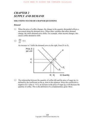
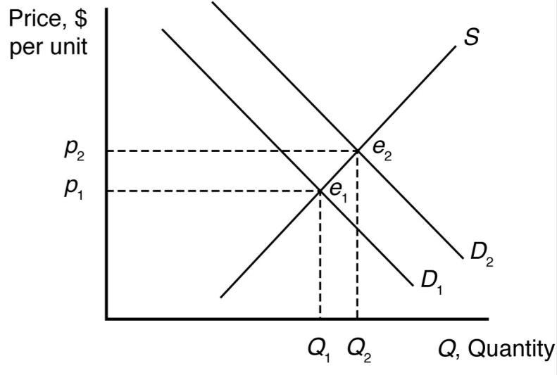
An increase in Y shifts the demand curve to the right, from D1 to D2
1.3 The relationship between the quantity of coffee (��) and the price of sugar (����) is defined by the coefficient on the ���� term in the equation. Since this coefficient is negative (it’s value is 0.3), an increase in the price of sugar (����) will decrease the quantity of coffee. This is the definition of a complementary good. More
specifically, if the price of sugar goes up by $1.00 per pound, then the demand for coffee will fall by 300,000 tons.
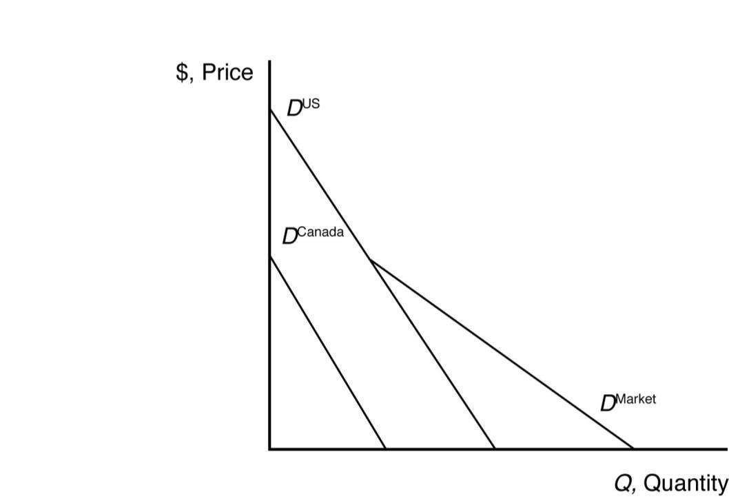
1.4 The market demand curve is the sum of the quantity demanded by individual consumers at a given price. Graphically, the market demand curve is the horizontal sum of individual demand curves.
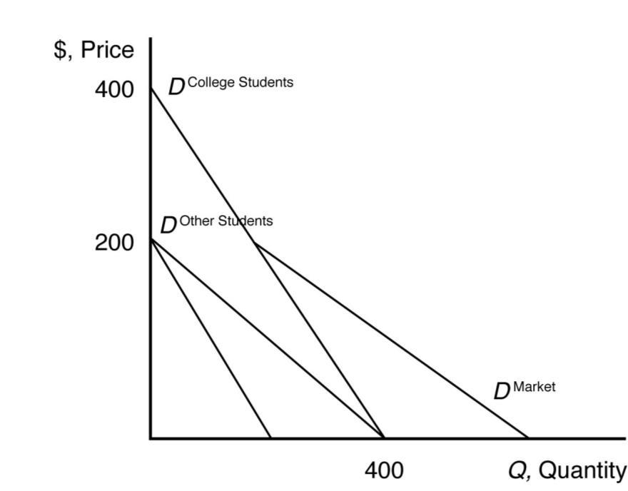
1.5 a. The inverse demand curve for other town residents is p = 200 0.5Qr.
b. At a price of $300, college students demand 100 units of firewood, and other residents demand no firewood. Other residents will demand zero units of firewood if the price is greater than or equal to $200.
c. The market demand curve is the horizontal sum of individual demand curves, as illustrated below.
Supply
2.1 The effect of a change in pf on Q is f p Q = 20pf f p Q
= 20(1.10)
= −22 units.
Thus, an increase in the price of fertilizer will shift the avocado supply curve to the left by 22 units at every price (i.e., a parallel shift to the left).
2.2 When the price of avocados changes, the change in the quantity supplied reflects a movement along the supply curve. When costs or other variables that affect supply change, the entire supply curve shifts. For example, the price of fertilizer represents a key factor of avocado production, which affects the cost of avocado production, shifting the avocado supply curve. This is because avocado prices are measured on a graph axis. Other factors that affect supply are not measured by a graph axis.
2.3 Given the supply function, Q = 58 + 15p–20pf,
The effect of a change in p on Q is
15p.
To change quantity by 60, price would need to change by 60 = 15p p = $4.00.
2.4 The market supply curve is the sum of the quantity supplied by individual producers at a given price. Graphically, the market supply curve is the horizontal sum of individual supply curves.
Market Equilibrium
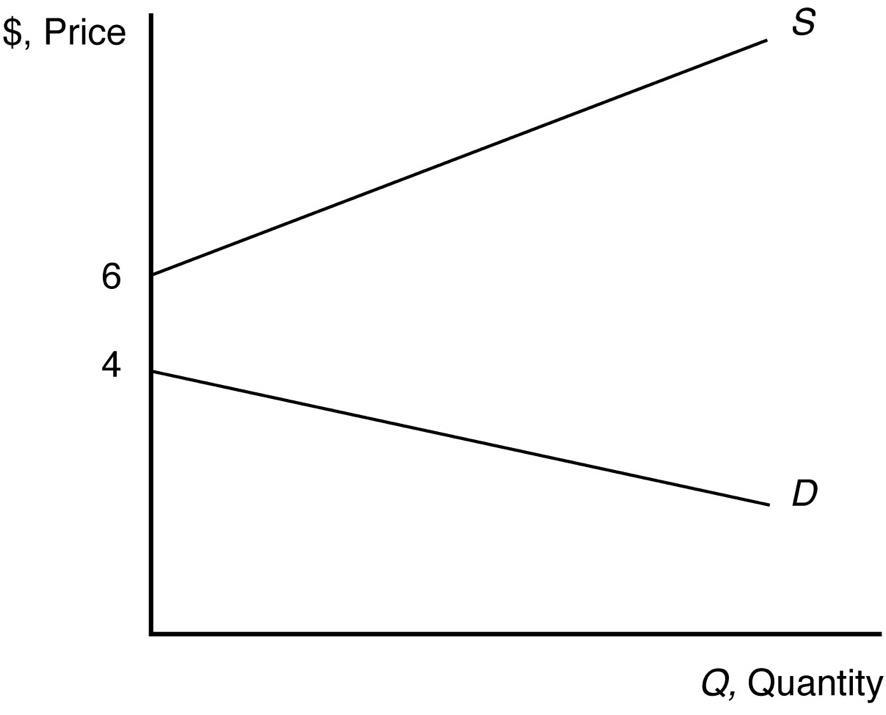
3.1 The supply curve is upward sloping and intersects the vertical price axis at $6. The demand curve is downward sloping and intersects the vertical price axis at $4. When all market participants are able to buy or sell as much as they want, we say that the market is in equilibrium: a situation in which no participant wants to change its behavior. Graphically, a market equilibrium occurs where supply equals demand. An equilibrium does not occur at a positive quantity because supply does not equal demand at any price.
3.2 The equilibrium price is p = $300, and the equilibrium quantity is Q = 2000.
3.3 Given that ps = $0.20, pc = $5, and Y = $55,000 (note Y is measured in thousands, so the value to use here is 55), the demand for coffee can be rewritten as Q = 14 p and the supply of coffee can be rewritten as Q = 8.6 + 0.5p.
When all market participants are able to buy or sell as much as they want, we say that the market is in equilibrium: a situation in which no participant wants to change its behavior. Graphically, a market equilibrium occurs where supply equals demand. Thus, the equilibrium price is D = S
14 p = 8.6 + 0.5p
5.4 = 1.5p p = $3.60.
Find the equilibrium quantity by substituting this price into either the supply or demand function. For example, using the supply function, the equilibrium quantity is
Q = 8.6 + 0.5p
Q = 8.6 + 0.5(3.60)
Q = 8.6 + 1.8
Q = 10.4 units.
3.4 If Y = $55,000, ps = 0.20, pc = $5, and p = 4, the quantity demanded is Q = 8.56 4 0.3(0.2) + 0.1(55) = 10. The quantity supplied is Q = 9.6 + 0.5(4) 0.2(5) = 10.6. There is an excess supply equal to 10.6 10.0 = 0.6 in this case. Because of the excess supply, firms unable to sell at the price of $4 would lower their prices, forcing the market price down. Price would fall until the equilibrium price was reached.
Shocks to the Equilibrium
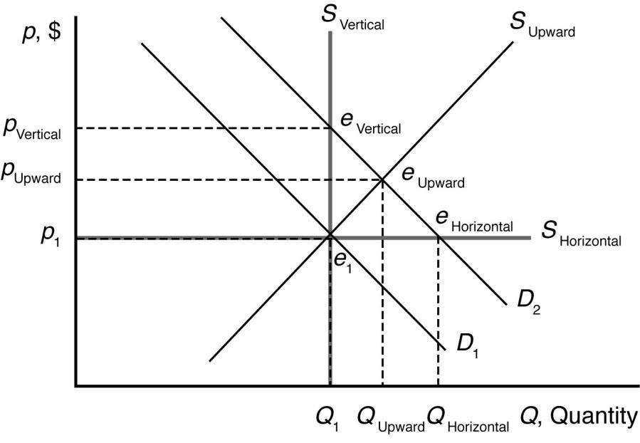
4.1 a. The new equilibrium with the horizontal supply curve is where the new demand curve intersects the horizontal supply curve. The new equilibrium price is unchanged. See figure.
b. The new equilibrium with the vertical supply curve is where the new demand curve intersects the vertical supply curve. The new equilibrium price is higher. See figure.
c. The new equilibrium with the upward-sloping supply curve is where the new demand curve intersects the upward-sloping supply curve. The new equilibrium price is higher. See figure.
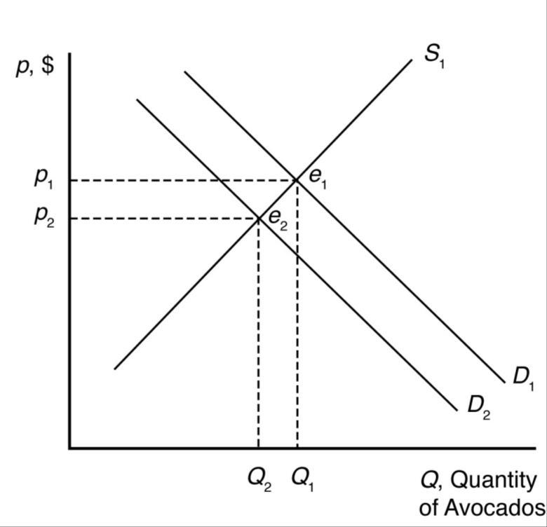
4.2 a. Health benefits from drinking coffee shift the demand curve for coffee to the right because more coffee is now demanded at each price. The new market equilibrium is where the original supply curve intersects the new coffee demand curve, at a higher price and larger quantity.
b. An increase in the usefulness of cocoa will increase demand for cocoa. This will drive up the equilibrium price of cocoa. Since cocoa and coffee are likely substitutes, this will increase the demand for coffee. The new market equilibrium is where the original supply curve intersects the new coffee demand curve, at a higher price and higher quantity.
c. A recession shifts the demand curve for coffee to the left because less coffee is now demanded at each price. The new market equilibrium is where the original supply curve intersects the new coffee demand curve, at a lower price and lower quantity.
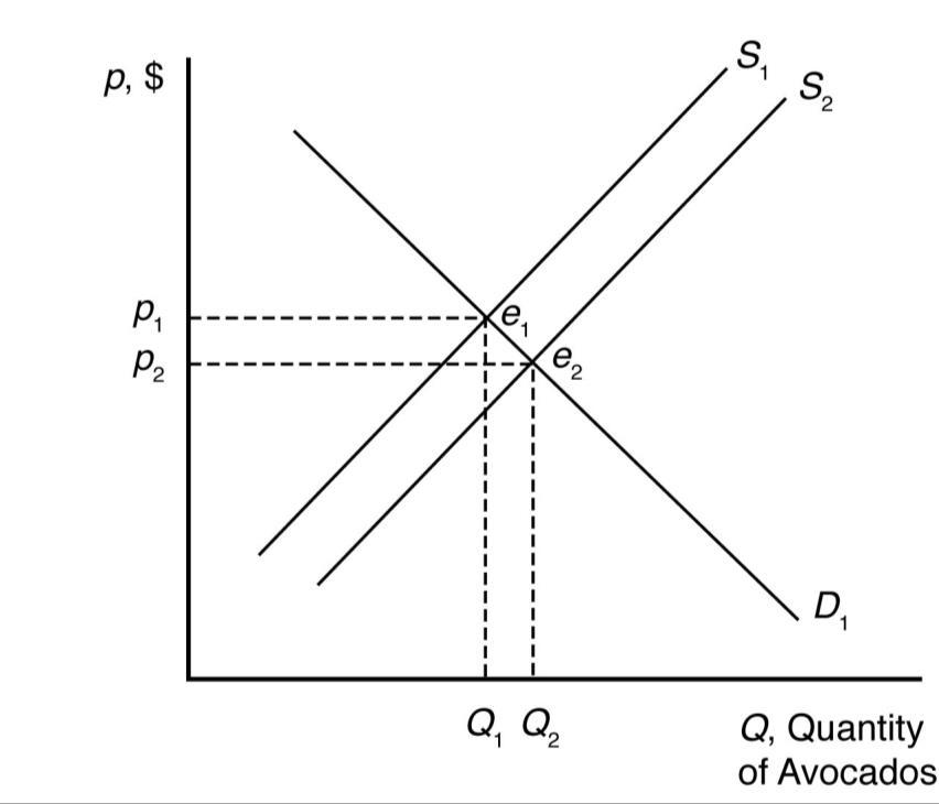
d. New technologies increasing yields shift the supply curve for coffee to the right because more coffee is now supplied at each price. The new market equilibrium is where the original demand curve intersects the new avocado supply curve, at a lower price and higher quantity.
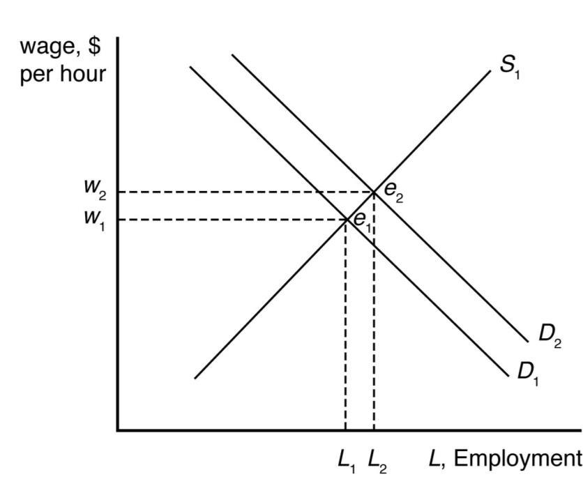
4.3 Outsourcing shifts the labor demand curve to the right because more Indian workers are demanded at each wage. The new market equilibrium is where the original supply curve intersects the new labor demand curve.
4.4 Given that pt = $0.80, the demand for avocados can be rewritten as Q = 160 40p and the supply of avocados can be rewritten as Q = 50 + 15p
When all market participants are able to buy or sell as much as they want, we say that the market is in equilibrium: a situation in which no participant wants to change its behavior. Graphically, a market equilibrium occurs where supply equals demand. Thus, the equilibrium price is D = S
160 40p = 50 + 15p
110 = 55p p = $2.00.
Find the equilibrium quantity by substituting this price into either the supply or demand function. For example, using the supply function, the equilibrium quantity is
Q = 50 + 15p
Q = 50 + 15(2.00)
Q = 50 + 30
Q = 80 units.
When the price of tomatoes increases to $1.35, the demand curve for avocados shifts out to
Q = 171 40p
The supply of avocados is unchanged. The new equilibrium is found where D = S
171 40p = 50 + 15p
121 = 55p p = $2.20.
The equilibrium quantity is found as before
Q = 50 + 15p
Q = 50 + 15(2.20)
Q = 50 + 33
Q = 83 units.
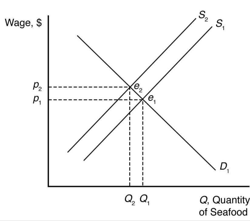
4.5 A leftward shift in the labor supply curve will drive up wages and reduce employment. The size of these effects will depend on the relative slopes of the supply and demand curves for labor.
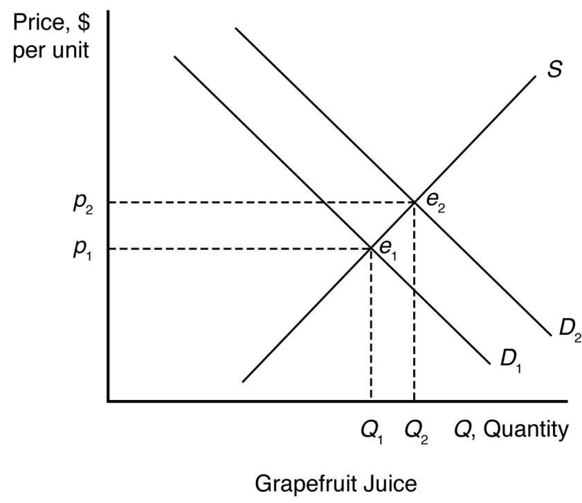
4.6 The damage reduces the supply of oranges, increasing the equilibrium price and decreasing the equilibrium quantity of orange juice.
The demand for grapefruit juice increases as the price of orange juice increases because grapefruit juice is a substitute. As the demand for grapefruit juice increases, the equilibrium price and quantity of grapefruit juice increase.
4.7 The increased use of corn for producing ethanol will shift the demand curve for corn to the right. This increases the price of corn overall, reducing the consumption of corn as food.
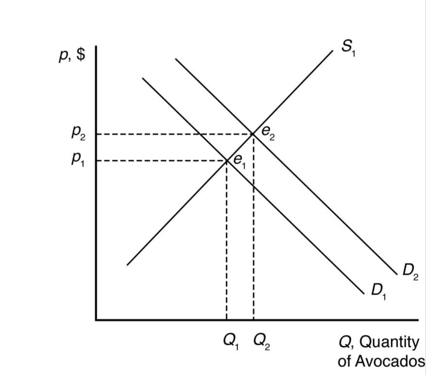
4.8 Suppose supply is initially S1, but it decreases by a small amount to S2 after the BP oil spill. When all market participants are able to buy or sell as much as they want, we say that the market is in equilibrium: a situation in which no participant wants to change its behavior. Graphically, a market equilibrium occurs where supply equals demand. The original market equilibrium is where the original demand curve intersects the original supply curve (e1). The new market equilibrium is where the original demand curve intersects the new supply curve (e2). When the supply curve shifts by a relatively small amount, the change in the equilibrium price is likely to be small.
4.9 Concerns about botulism caused the demand curve for baby formula to shift in. (A lower quantity was demanded at any given price.) This demand curve shift would put downward pressure on price and quantity. The removal of production permits caused the supply curve to shift in. (A lower quantity was supplied at any given price.) This supply curve shift would put upward pressure on price and downward pressure on quantity. Overall, the price could rise or fall depending on the relative size of the demand curve and supply curve shifts. However, quantity would have to fall.
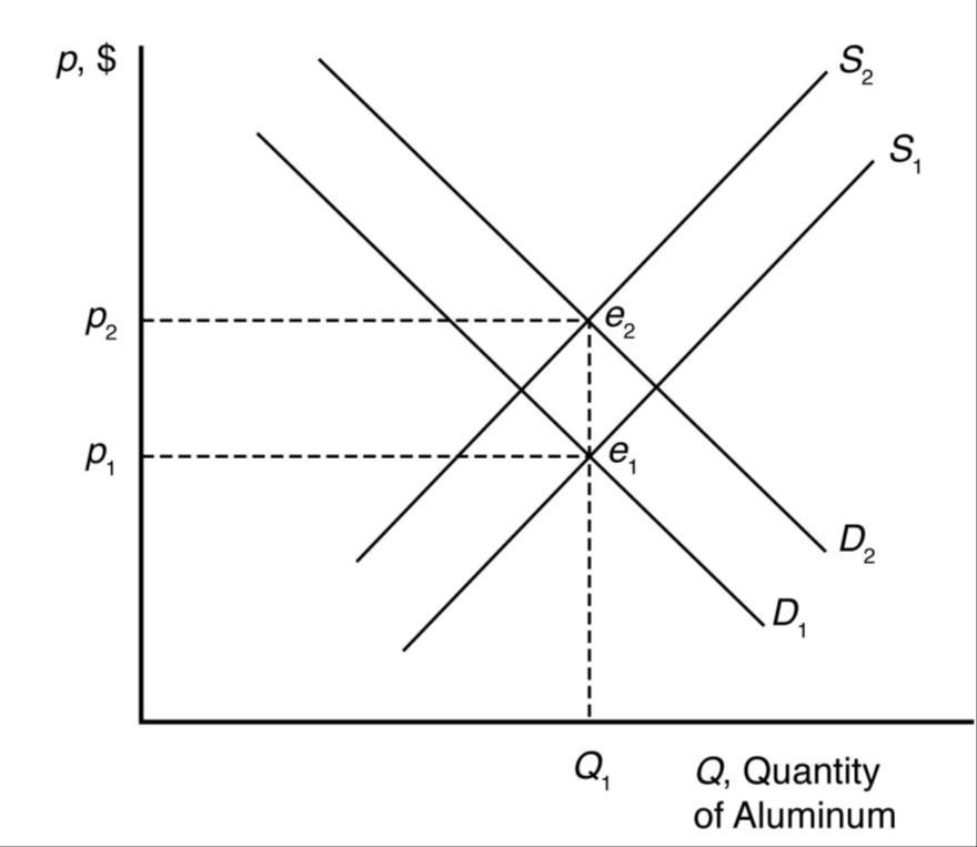
4.10 An increase in petroleum prices shifts the aluminum supply curve to the left because the cost of producing aluminum is more expensive at each price. An increase in the cost of petroleum also shifts the demand curve for aluminum to the right because the petroleum price increase makes a substitute, plastic, more expensive (by making the cost of plastic production higher). The new equilibrium is where the new aluminum supply curve intersects the new aluminum demand curve. When the supply curve shifts to the left, the new equilibrium price is higher and the new equilibrium quantity is lower. When the demand curve shifts to the right, the new equilibrium price is higher and the new equilibrium quantity is higher. When both curves shift, the new equilibrium price is higher, but the new equilibrium quantity could be higher, lower, or unchanged.
4.11 The cartoon seems to show a bumper harvest of lobsters. A large increase in the catch will shift the supply curve to the right (from S1 to S2) which will cause price to fall from p1 to p2.
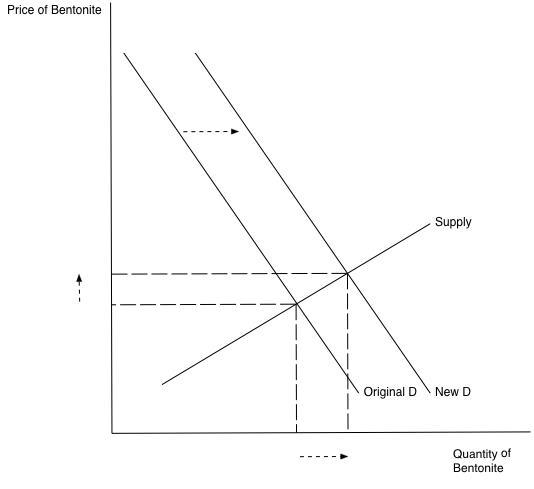
4.12 When drilling increases in response to the rising price of crude oil, the demand for bentonite increases as well. The demand curve will shift to the right and cause the equilibrium price and quantity of bentonite to increase. This is illustrated in the picture below:
Effects of Government Interventions
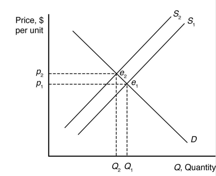
5.1 The effect of vendor licensing is to reduce the number of street vendors relative to the undistorted market equilibrium. Therefore, the number of handbags (and other products) offered for sale by street vendors is less than it would be without licensing (with free entry). As a result, the supply curve for handbags available from street vendors has shifted in compared with what it would be without licensing. The diagram representing the street vendor handbag market is therefore similar to the diagram in Q&A 2.2. The market price is higher and the quantity sold is lower than it would be without mandatory licensing.
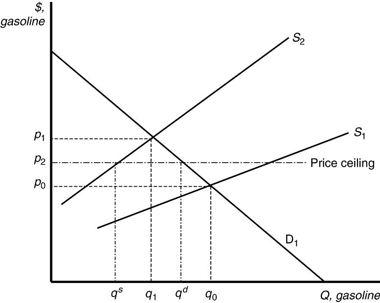
5.2 In the absence of price controls, the leftward shift of the supply curve as a result of Hurricane Katrina would push market prices up from p0 to p1 and reduce quantity from q0 to q1. At a government imposed maximum price of p2, consumers would want to purchase qd units, but producers would only be willing to sell qs units. The resulting shortage would impose search costs on consumers making them worse off. The reduced quantity and price also reduced firms’ profits.
5.3 With a binding price ceiling, such as a ceiling on the rate that can be charged on loans, some consumers who demand loans at the rate ceiling will be unable to obtain them. This is because the demand for bank loans is greater than the supply of bank loans to low-income households with the usury law.
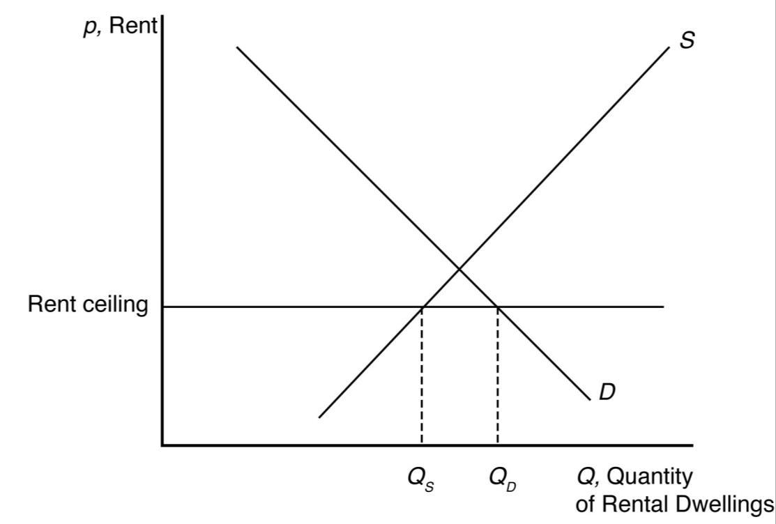
5.4 With the binding rent ceiling, the quantity of rental dwellings demanded is that quantity where the rent ceiling intersects the demand curve (QD). The quantity of rental dwellings supplied is that quantity where the rent ceiling intersects the supply
curve (QS). With the rent control laws, the quantity supplied is less than the quantity demanded, so there is a shortage of rental dwellings.
5.5 We can determine how the total wage payment, W = wL(w), varies with respect to w by differentiating. We then use algebra to express this result in terms of an elasticity:
where is the elasticity of demand of labor. The sign of dW/dw is the same as that of 1 + . Thus, total labor payment decreases as the minimum wage forces up the wage if labor demand is elastic, < –1, and increases if labor demand is inelastic, > –1.
For a graphical explanation, see the figures below. In the top panel with very flat supply and demand curves, the imposition of a minimum wage causes overall wage payments to fall dramatically. On the other hand, when supply and demand curves are steep (as in the bottom panel), overall wage payments increase substantially.
5.6 Before the tax is imposed, the demand for avocados can be rewritten as Q = 160 40p and the supply of avocados is given as Q = 50 + 15p.
When all market participants are able to buy or sell as much as they want, we say that the market is in equilibrium: a situation in which no participant wants to change
its behavior. Graphically, a market equilibrium occurs where supply equals demand. Thus, the equilibrium price is
D = S
160 40p = 50 + 15p 110 = 55p p = $2.00.
Find the equilibrium quantity by substituting this price into either the supply or demand function. For example, using the supply function, the equilibrium quantity is
Q = 50 + 15p
Q = 50 + 15(2.0)
Q = 50 + 30
Q = 80 units.
If a $0.55 tax is imposed, the demand curve can be rewritten to account for the tax. First, the demand curve can be rewritten as inverse demand by solving for p
Q = 160 40p
p = 4 0.025Q.
The tax is subtracted from inverse demand to give p = 3.45 0.025Q and then this inverse demand curve can be turned back into a demand curve
Q = 138 40p.
Setting supply equal to demand, the new equilibrium (pretax) price is
D = S
138 40p = 50 + 15p 88 = 55p p = $1.60.
The after-tax price is $2.15.
Using the supply function, the equilibrium quantity is
Q = 50 + 15p
Q = 50 + 15(1.60)
Q = 50 + 24
Q = 74 units.
5.7 a. If demand is vertical and supply is upward sloping, then all the tax burden is paid by consumers because they are not price sensitive.
b. If demand is horizontal and supply is upward sloping, then all the tax burden is paid by producers because consumers are infinitely price sensitive.
c. If demand is downward sloping and supply is horizontal, then all the tax burden is paid by consumers because producers are infinitely price sensitive.
5.8 If instead of the tax being levied on producers it is collected from consumers, then the effect will be a decrease in demand. The demand curve will shift left until the vertical distance between the original demand curve and the new one is equal to the tax of $2.40. This new demand curve, call it D2, will intersect the original supply curve (S1) at a price of $5.60 and a quantity of 11.6. In addition to the price of $5.60 per bushel, buyers will also have to pay the $2.40 tax for a total, after-tax price of $8.00. The seller will receive the $5.60 per bushel, and the government will collect $27.84 billion in tax revenue (the $2.40 tax multiplied by the 11.6 billion bushels of corn traded in the new equilibrium).
This equilibrium is not the same as the case in Q&A 2.3 because in that problem the supply curve is perfectly elastic, while in this case it is not. In Q&A 2.3, the seller passes on the entire tax to consumers, while here, the tax is split with $0.80 being paid by consumers and $1.60 paid by producers.
5.9 A tax on consumers will undoubtedly shift the demand curve down by an amount equal to the size of the tax. The new equilibrium price and quantity with the tax will be where the new demand curve intersects the original supply curve. The decrease in quantity will be larger (and tax revenue smaller) the more horizontal the supply curve is. Just the opposite is true if the supply curve is more vertical quantity effects will be small, and revenue generation from the tax will be large.
When to Use the Supply-and-Demand Model
6.1 The supply-and-demand model is accurate in perfectly competitive markets, which are markets in which all firms and consumers are price takers: no market participant can affect the market price. If there is only one seller of a good or service a monopoly that seller is a price taker and can affect the market price. Firms are also price setters in an oligopoly a market with only a small number of firms. Experience has shown that the supply-and-demand model is reliable in a wide range of markets, such as those for agriculture, financial products, labor, construction, many services, real estate, wholesale trade, and retail trade.
Managerial Problem
7.1 A tax paid by consumers shifts the demand curve down by an amount equal to the size of the tax. Just the opposite, suspending a tax on consumers should raise the demand curve by an amount equal to the size of the suspended tax. Although fuel supply is more likely to be vertical in the short run than in the long run, equilibrium fuel prices will increase when the demand curve shifts up whether the supply curve is vertical or upward sloping.
SOLUTIONS TO SPREADSHEET EXERCISES
Solutions Available on MyLab Economics
CHAPTER 2
Supply and Demand
CHAPTER OUTLINE
ManagerialProblem:CarbonTaxes
2.1Demand
TheDemandCurve
EffectsofaPriceChangeontheQuantityDemanded EffectsofOtherFactorsonDemand
TheDemandFunction
UsingCalculus:DerivingtheSlopeofaDemandCurve
SummingDemandCurves
Mini-Case:SummingCornDemandCurves
2.2Supply
TheSupplyCurve
EffectsofPriceonSupply
EffectsofOtherVariablesonSupply
TheSupplyFunction
SummingSupplyCurves
2.3MarketEquilibrium
UsingaGraphtoDeterminetheEquilibrium
UsingMathtoDeterminetheEquilibrium
ForcesThatDrivetheMarkettoEquilibrium
Mini-Case:SpeedofAdjustmenttoNewInformation
2.4ShockstotheEquilibrium
EffectsofaShiftintheDemandCurve
Q&A2.1
EffectsofaShiftintheSupplyCurve
Mini-Case:TheOpioidEpidemicReducesLaborMarketParticipation
Q&A2.2
ManagerialImplication:TakingAdvantageofFutureShocks
2.5EffectsofGovernmentInterventions
PoliciesThatShiftCurves
Mini-Case:OccupationalLicensing
PriceControls
PriceCeilings
Mini-Case:VenezuelanPriceCeilingsandShortages
PriceFloors
WhySupplyNeedNotEqualDemand
SalesTaxes
EquilibriumEffectsofaSpecificTax Pass-Through
Q&A2.3
ManagerialImplication:CostPass-Through
2.6WhentoUsetheSupply-and-DemandModel
ManagerialSolution:CarbonTaxes
MAIN TOPICS
1. Demand: Thequantityofagoodorservicethatconsumersdemanddependson priceandotherfactorssuchasconsumerincomesandthepricesofrelatedgoods.
2. Supply: Thequantityofagoodorservicethatfirmssupplydependsonpriceand otherfactorssuchasthecostofinputsandtheleveloftechnologicalsophistication usedinproduction.
3. Market Equilibrium: Theinteractionbetweenconsumers’demandand producers’supplydeterminesthemarketpriceandquantityofagoodorservice thatisboughtandsold.
4. Shocks to the Equilibrium: Changesinafactorthataffectdemand(suchas consumerincome)orsupply(suchasthepriceofinputs)alterthemarketpriceand quantitysoldofagoodorservice.
5. Effects of Government Interventions: Governmentpolicymayalsoaffectthe equilibriumbyshiftingthedemandcurveorthesupplycurve,restrictingpriceor quantity,orusingtaxestocreateagapbetweenthepriceconsumerspayandthe pricefirmsreceive.
6. When to Use the Supply-and-Demand Model: Thesupply-and-demandmodel appliesverywelltohighlycompetitivemarkets,whicharetypicallymarketswith manybuyersandsellers.
OVERVIEW
Thisisobviouslyanimportantchapterandwhilemuchofthismaterialwillbe reviewformanystudents,agood,solidunderstandingofthebasicsherewillpaybig dividendslater.
Demand: Thisisagoodplacetobeginsincemoststudentshaveexperiencethinking aboutmarketsituationsfromtheperspectiveofaconsumer. Whetherstudents havebeenexposedtothismaterialpreviouslyornot,oneofthetrickiestpartsin thissectionisthedistinctionbetweenachangeinpriceandachangeinanyofthe otherdeterminantsofdemand. Theformer,ofcourse,leadstoachangeinquantity demandedandamovementalongthedemandcurve,whilethelatterleadstoa changeindemandandashiftoftheentiredemandcurve. Itishelpfultopointout thatthisdistinctionissomewhatartificialandisdrivenbythefactthatthedemand relationshipisbeingrepresentedgraphicallyintwodimensions. Dependingonthe mathematicalpreparationoftheclass,itcanbeveryhelpfultodiscussthedemand relationshipalgebraicallywithoutworryingaboutdrawingthediagram. Thisallows formultipleright-handsidevariablesinthedemandfunctionandnoconcernabout whichoneleadstowhichtypeofchange. Forsomestudents,thiscanbeaneyeopeningobservation.
Supply: Thediscussionhereparallelsthediscussioninthesectionondemand. The biggestdifferenceisthatstudentsarenotasfamiliarwithtakingtheperspectiveofa producer,andsoadditionaldiscussionmightbenecessarytogetthemthinkingin thisway. Thesametechnicalconcernariseswithashiftinthesupplycurveversusa movementalongthecurve,butitcanbehandledthesamewaythatitwasin discussingdemand.
Market Equilibrium: Ifthereisoneresultthatstudentsarelikelytorecallfrompast coursework,itisthefactthattheintersectionofthesupplyanddemandcurves markstheequilibriumpointinthemarket. Despitethisfamiliarity,however,itis importanttotakethetimetoworkthroughanypartsofthediscussionthatarenew (eg.,solvingforequilibriumpriceandquantityalgebraically).
Itisofteneasiertoremindstudentsofwhytheintersectionofsupplyanddemandis theequilibriumbyconsideringpricesthatarebothhigherandlower. Labelthe (potential)equilibriumpriceinthediagramandthenaskstudentstothinkabout highprices(thoseabovethisproposedvalue)andlowprices(thosebelowthis value). Itshouldberelativelyeasyforstudentstorecallandseethatathighprices thereisasurpluswherequantitysuppliedexceedsquantitydemanded. Italso shouldberelativelyeasyforthemtosuggestthatpricesshouldfallinthis circumstance. Likewise,atlowpricestherewillbeashortageasquantitydemanded exceedsquantitysupplied. Thisdisequilibriumshouldleadtorisingprices. This leavesonlythepointwherequantitysuppliedequalsquantitydemandedasthespot wherethereisnomarketpressureforpricestoriseorfall,i.e.,themarketisin equilibrium.
Shocks to the Equilibrium: Thisisthebasicstoryofcomparativestatics. Students probablywillbefamiliarwiththistypeofanalysisfromagraphical,qualitative perspective,butitisagoodideatospendsometimeshowingthemhowthesame analysiscanbecomemorequantitativeinthepresenceofspecificfunctionalforms forsupplyanddemand. Thisisanopportunitytopracticesomebasicalgebraskills andalsoservesasmotivationfortheestimationofdemandandsupplyfunctions thatwillbecomingupinChapter3.
Effects of Government Interventions: Therearetwotopicshere:priceceilingsand floorsandsalestaxes. Thediscussiononpriceceilingsandfloorsshouldbepretty straightforwardafterdiscussingequilibriumandwhypricesaboveandbelow marketequilibriumarenotbalanced. Aneffectivepriceceilingorflooressentially createsapersistentdisequilibriumwitharesultingexcessshortageorsurplus. Care shouldbetakentoemphasizethatnotallpriceceilingsandfloorsresultin disequilibriumandthatitisimportanttocomparethepricerestrictiontotheactual marketequilibriumtodeterminewhethertherewillbeanyeffect.
Thediscussiononsalestaxesislessintuitiveandoftentakesworkforstudentsto understand. Thekeyresultisthattheeffectoftaxisdeterminedsolelybythe natureofsupplyanddemandandnotbytheadministrativedecisionaboutwho shouldremitthetaxtothetaxingauthority. Perhapsthemosteffectivewaytomake thispoint(anditprovidesgoodpracticeaswell)istoworkthroughanumerical example. Italsocanbehelpfulforstudentstoworkoutanddiscusstheresultsof taxesimposedinmarketswithextremesupplyanddemandrelationships(vertical orhorizontalsupplyand/ordemandcurves).
When to Use the Supply-and-Demand Model: Thisshortsectionmakesthe importantpointthatnotallmarketsituationsaresuitableforanalysiswiththe supply-and-demandmodel. Takingafewminutestopointoutthatthismodelisa descriptionofacompetitivemarketwillhelpstudentsavoidthecommonmistakeof misapplyingtheseresultslateron.
TEACHING TIPS
Is This Economics or Chemistry? Oneofmyfavoriteexamplestousewhen teachingaboutequilibriumandcomparativestaticsinthesupplyanddemand modelinvolvesatripdownmemorylane. Itellstudentsthestoryofmyfirst chemistrylabasayoungladinhighschool. Whatwassointerestingaboutthislab experience,andthewayitrelatestoteachingaboutequilibrium,isthattheexercise involvedaperiodofgreatdisequilibrium. Inthechemistryexperiment,this disequilibriumtooktheformofabubbling,stinkyliquid. Theexperimentstarted withallthechemicalsinequilibrium–abeakerwithaclearliquid,atesttubewitha graypowder,etc. Thetaskforthelabwastomixthemtogetherand,basedonthe changesthatoccurred,determinetheidentityofeachoftheoriginalcomponents. So,initialequilibriumwasfollowedbybubblingandstinkywhich,inturn,was followedbyanewequilibrium. Wethencomparedthestartingpointtotheending point essentiallydoingcomparativestaticsinchemistrylab.
A Classroom Experiment Thistopicmorethananyotherinthecourselendsitself toademonstrationintheformofaclassroomexperiment. Therearemanydifferent waystogivestudentstheexperienceofseeinganequilibriumpriceandquantity develop,butoneofmyfavoritesisonefromCharlieHolt(Holt,CharlesA. “ClassroomGames:TradinginaPitMarket,”JournalofEconomicPerspectives,10:1 (Winter1996),193-203). Thebeautyofanexerciselikethisisthatitgivesstudents theopportunitytoreallyfeelmarketforcesatwork. Youcanspiceupthe experimentbybringingalongsomeprizes(candybarsworkwell)togeteveryone motivatedtoplayseriously.
ADDITIONAL DISCUSSION QUESTIONS
1. Explainwhythedifferencebetweenashiftinthedemandcurveandmovement alongthedemandcurveissoimportant. Explainwhyitbecomeslessimportant onceweleavetwo-dimensionaldiagramsbehind.
2. Canyouthinkofexamplesoftaxesthatarelargelypaidforbyconsumers? What aboutthosethatarelikelytobepaidforbyproducers? Explainwhywhopaysis differentfromwhoisresponsibleforsendingthetaxmoneyofftothetaxing authority.
3. Giveanexampleofamarketthatislikelytobesimilartothesupplyanddemand modelpresentedhere. Howaboutonethatisverydifferent?
4. Whatsalesandincometaxratesinyourstate?Whatwouldhappenifthesetaxes werereducedandacarbontaxtooktheirplace?Doyouthinkthisisagoodidea?
Managerial Economics and Strategy
ThirdEdition

Chapter 2
Supply and Demand
Managerial Problem
Carbon Taxes
• What will be the effect of imposing a carbon tax on the price of gasoline
Solution Approach
• Managers use the supply-and-demand model to answer this type of questions.
Model
• The supply-and-demand model provides a good description of many markets and applies particularly well to markets in which there are many buyers and many sellers.
• In markets where this model is applicable, it allows us to make clear, testable predictions about the effects of new taxes or other shocks on prices and other market outcomes.
Learning Objectives (1
of 2)
2.1 Demand
Explain how the quantity of a good or service that consumers want depends on its price and other factors
2.2 Supply
Describe how the quantity of a good or service that firms want to sell depends on its price and other factors
2.3 Market Equilibrium
Show how the interaction between consumers’ demand and producers’ supply determines the market price and quantity
Learning Objectives
(2 of 2)
2.4
Shocks to the Equilibrium
Predict how an event that affects consumers or firms changes the market price and quantity
2.5 Effects of Government Interventions
Analyze the market effects of government policy using the supply-and-demand model
2.6 When to Use the Supply-and-Demand Model
Discuss when to use the supply-and-demand model
2.1 Demand (1 of 7)
• Consumers decide whether to buy a particular good or service.
– If they decide to buy, how much is based on its own price and on other factors.
• Own Price
– Economists focus most on how a good’s own price affects the quantity demanded.
– To determine how a change in price affects the quantity demanded, economists ask what happens to quantity when price changes and other factors are held constant.
• Other Factors
– The list of other factors usually includes income, price of related goods, tastes, information, government regulation.
– Go to next slide for more detail about these other factors of demand
2.1 Demand
(2 of 7)
• Other factors of demand include the following:
– Income
▪ When a consumer’s income rises that consumer will often buy more of many goods.
– Price of related goods
▪ Substitute: Different brands of essentially the same good are close substitutes.
▪ Complement: is a good that is used with the good under consideration.
– Information
▪ Information about characteristics and the effects of a good has an impact on consumer decisions
– Tastes
▪ Consumers do not purchase goods they dislike. Firms devote significant resources to trying to change consumer tastes through advertising.
– Government Regulations
▪ Governments may ban, restrict, tax, or subsidize goods or services
2.1 Demand
The Demand Curve
(3 of 7)
• A demand curve shows the quantity demanded at each possible price, holding constant the other factors that influence purchases.
• The quantity demanded is the amount of a good that consumers are willing to buy at a given price, holding constant the other factors that influence purchases.
• Graphical Presentation
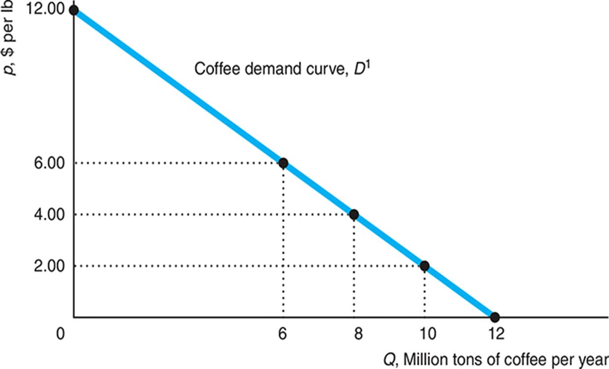
– In Figure 2.1, the demand curve hits the vertical axis at $12, indicating that no quantity is demanded when the price is $12 per lb or higher.
– The demand curve hits the horizontal quantity axis at 12 million lbs, the quantity of avocados that consumers would want if the price were zero.
– The quantity demanded at a price of $2 per lb is 10 million lbs per year.
Figure 2.1 A Demand Curve
2.1
Demand
(4 of 7)
Effects of a Price Change on the Quantity Demanded
• The Law of Demand states that consumers demand more of a good if its price is lower or less when its price is higher.
– The law of demand assumes income, the prices of other goods, tastes, and other factors that influence the amount they want to consume are constant.
– The law of demand is an empirical claim—a claim about what actually happens.
– According to the law of demand, demand curves slope downward, as in Figure 2.1.
• The demand curve is a concise summary of the answer to the question: What happens to the quantity demanded as the price changes, when all other factors are held constant?
– Changes in the quantity demanded in response to changes in price are movements along the demand curve.
2.1
Demand
(5 of 7)
Effects of Other Factors on Demand
• A change in any relevant factor other than the price of the good causes a shift of the demand curve rather than a movement along the demand curve.
• Example and Figure 2.2:
– If average family income goes up from $35,000 to $50,000, the global demand for coffee shifts to the right from 12Dto D.
– The price remains at $2 per pound, but the quantity demanded increases from 10 to 11.5 million pounds per year.
– Verify the same shift of demand would occur if the price of a substitute of coffee, say tea, goes up.
Figure 2.2 A Shift of the Demand Curve
2.1
Demand
(6 of 7)
The Demand Function: , (,) s QDppY
• Q of coffee demanded is a function of its price p, price of sugar ps and income Y. Other factors are constant.
• Estimated Demand Function: Q = 8.56 − p − 0.3ps + 0.1Y
– This specific linear form reflects empirical evidence; p and ps are negative and Y is positive. The constant term, 8.56, represents all other factors.
• Demand Curve: Q = 12 − p
– Straight-line demand curve 1D in Figure 2.1 with ps = 0.20, Y = 35. Notice that ΔQ =−Δp. So, if Δp = −$2, then 2 ( 2) Q million tons per year.
• The Law of Demand and Calculus
– The Law of Demand states that the derivative of the demand function with respect to price is negative, d/d0. Qp
– The demand function for coffee: Q = 12 − p. So, the derivative of the demand with respect to price: d/d1. Qp
2.1
Demand
(7 of 7)
Summing Demand Curves
• The overall demand for coffee is composed of the demand of many individual consumers.
• The total quantity demanded at a given price is the sum of the quantity each consumer demands at that price.
• We can generalize this approach to look at the total demand for more than two consumers, or we can apply it to groups of consumers rather than just to individuals.
2.2 Supply
(1 of 7)
• Firms determine how much of a good to supply on the basis of the price of that good and on other factors, including the costs of producing the good.
• Own Price
– Usually, we expect firms to supply more quantity at a higher price.
• Other Factors
– These other factors usually include costs of production, technological change, government regulations, and other factors.
– Go to next slide for more detail about these other supply factors.
2.2 Supply
(2 of 7)
• Costs of Production
– The costs of labor, machinery, fuel, and other costs affect how much of a product firms want to sell.
– As a firm’s cost falls, it is usually willing to supply more, holding price and other factors constant.Conversely, a cost increase will often reduce a firm’s willingness to produce.
• Technological Change
– If a technological advance allows a firm to produce its good at lower cost, the firm supplies more of that good at any given price, holding other factors constant.
• Government Regulations
– Government rules and regulations can affect supply directly without working through costs.
– For example, in some parts of the world, retailers may not sell most goods and services on particular days of religious significance.
2.2 Supply
The Supply Curve
(3 of 7)
• A supply curve shows the quantity supplied at each possible price, holding constant the other factors that influence firms’ supply decisions.
• The quantity supplied is the amount of a good that firms want to sell at a given price, holding constant other factors that influence firms’ supply decisions, such as costs and government actions.
• Graphical Presentation
– In Figure 2.3, the price on the vertical axis is measured in dollars per physical unit (dollars per lb), and the quantity on the horizontal axis is measured in physical units per time period (millions of tons per year).
– The quantity supplied at a price of $2 per lb is 10 million tons per year and 11 million tons per year when the price is $4.
Figure 2.3 A Supply Curve
2.2 Supply
(4 of 7)
Effects of Price on Supply
• The supply curve is usually upward sloping. There is no “Law of Supply” stating that the supply curve slopes upward.
• We observe supply curves that are vertical, horizontal, or downward sloping in particular situations. However, supply curves are commonly upward sloping.
• Along an upward-sloping supply curve, a higher price leads to more output being offered for sale, holding other factors constant.
• Changes in Quantity Supplied
– An increase in the price of avocados causes a movement along the supply curve, resulting in more coffee being supplied.
– As the price increases, firms supply more.
– In Figure 2.3, if the price rises from $2 per lb to $4 per lb, the quantity supplied rises from 10 to 11 million tons per year.
2.2 Supply
(5 of 7)
Effects of Other Variables on Supply
• A change in a relevant variable other than the good’s own price causes the entire supply curve to shift rather than a movement along the supply curve.
• Example and Figure 2.4:
– When the price of cocoa rises from $3 per lb to $6 per lb, many coffee farmers switch to producing cocoa. As a consequence, the supply curve for coffee shifts leftward, from 12 to SS (Figure 2.4).
– That is, firms want to supply less coffee at any given price than before the cocoa price increase. At a price of $2 per lb for coffee, the quantity supplied falls from 10 million lbs on 1S to 9.4 million tons on 2S (after the cocoa price increase).
Figure 2.4 A Shift of a Supply Curve
2.2 Supply
(6 of 7)
The Supply Function: (,) cQSpp
• Q of coffee demanded is a function of its price p and the price of cocoa pc. Other factors are constant.
• Estimated Supply Function: Q = 9.6 + 0.5p − 0.2pc
– This specific linear form reflects empirical evidence; p is positive and pc is negative. The constant term, 9.6, represents all other factors.
• Supply Curve: Q = 9 + 0.5p
– Straight-line supply curve 1S in Figure 2.3 with pc = $3. Notice that ΔS = 0.5Δp. So, if Δp = $1, then ΔS = 0.5 million tons per year.
– Thus, a $1 increase in price causes the quantity supplied to increase by 0.5 million tons per year.
– This change in q induced by a change in p is a movement along the supply curve.
2.2 Supply
(7 of 7)
Summing Supply Curves
• The total supply curve shows the total quantity produced by all suppliers at each possible price.
• In the coffee case, for example, the overall market quantity supplied at any given price is the sum of the quantity supplied by Brazilian, Vietnamese, Colombian, and other producers in various countries.
2.3 Market Equilibrium
(1 of 4)
• The D curve shows the q consumers want to buy at various p
• The S curve shows the q firms want to sell at various p
– The S and D curves jointly determine the p and q at which a good or service is bought and sold.
– The market is in equilibrium when all market participants are able to buy or sell as much as they want (no participant wants to change its behavior).
– The p at which consumers can buy as much as they want and sellers can sell as much as they want is an equilibrium price.
– The resulting q is the equilibrium quantity becausethe quantity demanded equals the quantity supplied.
2.3
Market Equilibrium
(2 of 4)
Using a Graph to Determine the Equilibrium
• In a graph, the market equilibrium is the point at which the demand and supply curves cross each other. This point gives the q and p of equilibrium.
• Graphical Presentation
– Figure 2.5 shows the supply curve, S, and demand curve, D, for coffee.
– The D and S curves intersect at point e, the market equilibrium.
– The equilibrium price is $2 per lb, and the equilibrium quantity is 10 million tons per year, which is the quantity firms want to sell and the quantity consumers want to buy.
Figure 2.5 Market Equilibrium
2.3 Market Equilibrium
Using Math to Determine the Equilibrium
(3 of 4)
• D and S Curves: Qd = 12 − p and Qs = 9 + 0.5p
– We want to find the p at which Qd = Qs = Q, the equilibrium quantity. In equilibrium, it must be that Qs = Qd.
• In Equilibrium Qd = Qs: 12 − p = 9 + 0.5p
– We use algebra to find the equilibrium price: 3 = 1.5p, so p = $2. We can determine the equilibrium q by substituting this p into either Qd or Qs.
• Using the D Curve: Q = 12 − 2 = 10
– We find that the equilibrium quantity is 10 million tons per year. We can obtain the same result if we use the S curve.
2.3 Market Equilibrium
Forces That Drive the Market to Equilibrium
Excess Demand
(4 of 4)
• Figure 2.5 shows the supply curve, S, and demand curve, D, for coffee.
• If the price of coffee were $1, firms are willing to supply 9.5 million tons per year but consumers demand 11 million tons. The market is in disequilibrium,andthereis excess demand…but not for long.
• Frustrated consumers may offer to pay suppliers more than $1 per lb and some suppliers might raise their prices. Such actions cause the market price to rise until it reaches the equilibrium price, $2 (excess D eliminated).
Excess Supply
• If instead the price were $3, firms are willing to supply 10.5 million tons per year but consumers demand 9 million tons. The market is in disequilibrium again, and there is excess supply…but not for long.
• To avoid unsold coffee to stale, firms lower the price to attract additional customers. The price falls until it reaches the equilibrium level, $2 (excess S eliminated and no more pressure to lower the price further).
2.4 Shocks to the Equilibrium (1 of 5)
• The D curve shows the q consumers want to buy at various p
• The S curve shows the q firms want to sell at various p
– The equilibrium changes only if a shock occurs that shifts the D curve or the S curve.
– These curves shift if one of the variables we were holding constant changes.
– If tastes, income, government policies, or costs of production change, the D curve or the S curve or both may shift, and the equilibrium changes.
2.4 Shocks to the Equilibrium (2
of 5)
Effects of a Shift in the Demand Curve
• Suppose that the average annual income in developed countries increases by $15,000 from $35,000 to $50,000, so consumers can buy more coffee at any given price. As a result, the demand curve for coffee shifts to the right from 12 to DD in Figure 2.6, panel (a).
– At the original equilibrium, e1, price is $2, and there is excess demand of 1.5 million lbs per month. Market pressures drive the price up until it reaches $3 at the new equilibrium, e2.
– Here the increase in income causes a shift of the demand curve, which in turn causes a movement along the supply curve from e1 to e2.
Figure 2.6 Equilibrium Effects of a Shift of a Demand or Supply Curve
2.4 Shocks to the Equilibrium (3 of 5)
Effects of a Shift in the Supply Curve
2.4
Shocks
to the Equilibrium (4 of 5)
Effects of a Shift in the Supply Curve
• Assuming that income remains at its $35,000 original level, an increase in the price of cocoa from $3 to $6 per lb causes some coffee producers to switch to cocoa production. So there are fewer suppliers and less coffee at every price. The supply curve for coffee shifts to the left from 12to,SS in Figure 2.6, panel (b).
– At the original equilibrium, e1, price is $2 per lb, and there is excess demand of 0.6 million tons per year. Market pressures drive the price up until it reaches $2.40 at the new equilibrium, e2.
– Here, a shiftof the supply curve results in a movementalong the demand curve.
2.4
Shocks to
the Equilibrium (5 of 5)
Managerial Implication: Taking Advantage of Future Shocks
• Managers can use the supply-and-demand model to anticipate how shocks to supply or demand will affect future business conditions and can take advantage of that knowledge.
– Mars is one of the world’s largest chocolate producers and managers use a supply-and-demand model to make cocoa buying decisions.
– If they expect prices to increase substantially, they immediately buy a great deal of cocoa at relatively low prices directly from suppliers in Africa.
– Alternatively, if they expect prices to fall, they may hold off buying now and then buy later at a lower price from organized markets such as ICE Futures U.S. or the London International Financial Futures and Options Exchange.
2.5 Effects of Government Interventions
(1 of 6)
Policies that Shift Curves
• Limits on Who can Buy
– For example, governments usually forbid selling alcohol to young people. This decreases the quantity demanded at each price and thereby shifts the demand curve to the left.
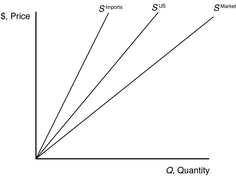
• Restriction of Imports
– The effect of this governmental restriction is to decrease the quantity supplied of imported goods at each price and shifts the importing country’s supply curve to the left.
• Start buying a good
– The effect of governments starting to buy goods is to increase the quantity demanded at each price for the good and shifts the demand curve to the right.
2.5 Effects of Government Interventions
(2 of 6)
Price Controls—Price Ceilings
• When the government sets a price ceiling at p and the unregulated equilibrium price is above it, the price that is actually observed in the market is the price ceiling.
– Price ceilings have no effect if they are set above the equilibrium price that would be observed in the absence of the price controls.
– In Figure 2.7, the new equilibrium gasoline price would be p2 but a price ceiling of p1 is imposed, then the ceiling price of p1 is charged.
• With a binding price ceiling, the supply-and-demand model predicts an equilibrium with a shortage:a persistent excess demand.
– The new equilibrium with a shortage in Figure 2.7 occurs with a quantity Qs and price p1 (the excess demand is Qs −Q1). If the price ceiling were removed, the new equilibrium would be e2.
– Deacon and Sonstelie (1989) found that for every dollar consumers saved during the 1980 gasoline price controls, they lost $1.16 in waiting time and other factors.
Figure 2.7 A Price Ceiling on Gasoline
2.5
Effects of
Government Interventions (3 of 6)
Price Controls—Price Floors
• When the government sets a price floor below the unregulated equilibrium price, the price that is actually observed in the market is the price floor.
– A minimum wage law forbids employers from paying less than the minimum wage, w.
• With a binding price floor, the supply-and-demand model predicts an equilibrium with a persistent excess supply.
– The minimum wage prevents market forces from eliminating this excess supply, so it leads to an equilibrium with unemployment.
– The new equilibrium with unemployment in Figure 2.8 occurs with a quantity Ld and wage w (the excess supply is Ls −Ld). If the price ceiling were removed, the new equilibrium would be e2
Figure 2.8 The Minimum Wage: A Price Floor
2.5 Effects of Government Interventions
(4 of 6)
Why Supply Need Not Equal Demand
• The theory says that the price and quantity in a market are determined by the intersection of the supply curve and the demand curve and the market clears if the government does not intervene.
• However, the theory also tells us that government intervention can prevent market clearing.
– The price ceiling and price floor examples show that the quantity supplied does not necessarily equal the quantity demanded in a supply-and-demand model.
– The quantity that sellers want to sell and the quantity that buyers want to buy at a given price need not equal the actual quantity that is bought and sold.
2.5 Effects of Government Interventions
(5 of 6)
Sales Taxes
Equilibrium Effects of a Specific Tax
• The specific sales tax causes the equilibrium price consumers pay to rise, the equilibrium quantity that firms receive to fall, and the equilibrium quantity to fall (p2, Q2, and T in Figure 2.9)
• Although the consumers and producers are worse off because of the tax, the government acquires new tax revenue, $27.84 billion in Figure 2.9.
Pass-Through
• Common Confusion: Businesses pass-through any sales tax to consumers, so that the price that consumers pay increases by the amount of the tax.
• This belief is not accurate in general. Full pass-through can occur, but partial passthrough is more common.
– In Figure 2.9, after a $2.40 specific tax is imposed on firms, the price consumers pay rises from $7.20 to $8.00. So, firms pass-through $0.80 to consumers and absorb $1.60 of the tax.
• The degree of the pass-through depends on the S and D shapes.
2.5 Effects of Government Interventions
(6 of 6)
Managerial Implication: Cost Pass-Through
• Managers should use pass-through analysis to predict the effect on their price and quantity from not just a new tax but from any per unit increase in costs.
– Suppose that the cost of producing corn rises $2.40 per bushel because of an increase in the cost of labor or other factors of production, rather than because of a tax.
– Then, the same analysis as in Figure 2.9 would apply, so a manager would know that only 80¢ of this cost increase could be passed through to consumers.
2.6 When to Use the Supply-AndDemand Model
(1 of 2)
• The Supply-and-Demand (S-D) model can help us to understand and predict real-world events in many markets. Like a map, it need not be perfect to be useful.
• The model is useful if the market to be analyzed is “competitive enough.”
• It is reliable in markets, such as those for agriculture, financial products, labor, construction, many services, real estate, wholesale trade, and retail trade.
• The S-D model is accurate for perfectly competitive markets.
– It is precisely accurate in perfectly competitive markets, which are markets in which all firms and consumers are price takers (no market participant can affect the market price).
– See next slide for characteristics of perfectly competitive markets.
• The S-D model is not accurate for noncompetitive markets.
• In markets with firms that are price setters, the market price is usually higher than that predicted by the S-D model.
– Monopoly and oligopoly markets have few sellers that are price setters. These markets need a different model.
2.6 When to Use the Supply-AndDemand
Model
(2 of 2)
• Five characteristics of a perfect competitive market:
– Many buyers and sellers, all relatively small with respect to the size of the market.
– Consumers believe all firms produce identical products, so they only care about price.
– All market participants have full information about price and product characteristics, so no participant can take advantage of each other.
– Transaction costs (expenses over and above the price) are negligible.
– Firms can easily enter and exit the market over time, so competition is very high.
Managerial Solution
Carbon Taxes
• What will be the effect of imposing a carbon tax on the price of gasoline?
Solution
• The degree to which a tax is passed through to consumers depends on the shapes of the demand-and-supply curves. Typically, short-run supply and demand curves differ from the long-run curves.
• In the long-run, the supply curve is upward sloping, as in our typical figure. However, the U.S. short-run supply curve of gasoline is very close to vertical.
• From empirical studies, we know that the U.S. federal gasoline specific tax of t = 18.4¢ per gallon is shared roughly equally between gasoline companies and consumers in the long run. However, based on what we learned, we expect that most of the tax will fall on firms that sell gasoline in the short run.
• Manufacturing and other firms that ship goods are consumers of gasoline. They can expect to absorb relatively little of a carbon tax when it is first imposed, but half of the tax in the long run.
opyghtCri


This work is protected by United States copyright laws and is provided solely for the use of instructors in teaching their courses and assessing student learning. Dissemination or sale of any part of this work (including on the World Wide Web) will destroy the integrity of the work and is not permitted. The work and materials from it should never be made available to students except by instructors using the accompanying text in their classes. All recipients of this work are expected to abide by these restrictions and to honor the intended pedagogical purposes and the needs of other instructors who rely on these materials.