Chapter 2: Analysis of Graphs and Functions
2.1: Graphs of Basic Functions and Relations; Symmetry
1. (,).
2. (,); [0,)
3. (0,0)
4. [0,); [0,)
5. increases
6. (,0]; [0,)
7. x-axis
8. even
9. odd
10. y-axis; origin
11. The domain can be all real numbers; therefore, the function is continuous for the interval (,) .
12. The domain can be all real numbers; therefore, the function is continuous for the interval (,) .
13. The domain can only be values where 0; x therefore, the function is continuous for the interval [0,).
14. The domain can only be values where 0; x therefore, the function is continuous for the interval (,0].
15. The domain can be all real numbers except 3; therefore, the function is continuous for the interval (,3)(3,).
16. The domain can be all real numbers except 1; therefore, the function is continuous for the interval (,1)(1,).
17. (a) The function is increasing for the interval 3,
(b) The function is decreasing for the interval ,3
(c) The function is never constant; therefore, none.
(d) The domain can be all real numbers; therefore, the interval (,).
(e) The range can only be values where 0; y therefore, the interval [0,).
18. (a) The function is increasing for the interval 4,
(b) The function is decreasing for the interval ,1
(c) The function is constant for the interval 1,4
(d) The domain can be all real numbers; therefore, the interval (,).
(e) The range can only be values where 3; y therefore, the interval [3,).
19. (a) The function is increasing for the interval ,1
(b) The function is decreasing for the interval 4,
(c) The function is constant for the interval 1,4
(d) The domain can be all real numbers; therefore, the interval (,).
(e) The range can only be values where 3; y therefore, the interval (,3].
20. (a) The function is never increasing; therefore, none.
(b) The function is always decreasing; therefore, the interval (,).
(c) The function is never constant; therefore, none.
(d) The domain can be all real numbers; therefore, the interval (,).
(e) The range can be all real numbers; therefore, the interval (,).
21. (a) The function is never increasing; therefore, none
(b) The function is decreasing for the intervals ,2 and 3,
(c) The function is constant for the interval (2,3).
(d) The domain can be all real numbers; therefore, the interval (,).
(e) The range can only be values where 1.5 y or 2; y therefore, the interval (,1.5][2,).
22. (a) The function is increasing for the interval (3,).
(b) The function is decreasing for the interval (,3).
(c) The function is constant for the interval 3,3
(d) The domain can be all real numbers except 3; therefore, the interval (,3)(3,).
(e) The range can only be values where 1; y therefore, the interval (1,).
23. Graph 5 ().fxx See Figure 23. As x increases for the interval (,), y increases; therefore, the function is increasing.
24. Graph 3 ().fxx See Figure 24. As x increases for the interval (,), y decreases; therefore, the function is decreasing.
25. Graph 4 ().fxx See Figure 25. As x increases for the interval ,0 y decreases; therefore, the function is decreasing on ,0
26. Graph 4 ().fxx See Figure 26. As x increases for the interval 0, , y increases; therefore, the function is increasing on 0, [-10,10] by [-10,10] [-10,10] by [-10,10] [-10,10] by [-10,10] [-10,10] by [-10,10] Xscl = 1 Yscl = 1 Xscl = 1 Yscl = 1 Xscl= 1 Yscl = 1 Xscl = 1 Yscl= 1

Figure 23
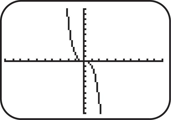
Figure 24

Figure 25
Copyright © 2019 Pearson Education, Inc.

Figure 26
27. Graph ()||.fxx See Figure 27. As x increases for the interval ,0, y increases; therefore, the function is increasing on ,0.
28. Graph ()||.fxx See Figure 28. As x increases for the interval 0, , y decreases; therefore, the function is decreasing on 0, .
29. Graph 3 (). fxx See Figure 29. As x increases for the interval (,), y decreases; therefore, the function is decreasing.
30. Graph (). fxx See Figure 30. As x increases for the interval 0, y decreases; therefore, the function is decreasing.
[-10,10] by [-10,10] [-10,10] by [-10,10] [-10,10] by [-10,10] [-10,10] by [-10,10]
Xscl = 1 Yscl = 1 Xscl = 1 Yscl = 1 Xscl= 1 Yscl = 1 Xscl = 1 Yscl= 1
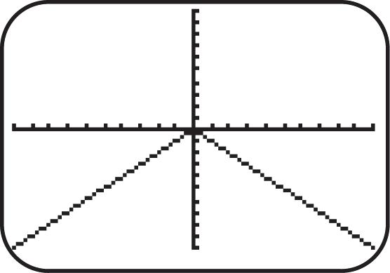
Figure 27
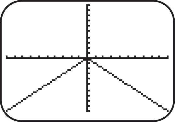
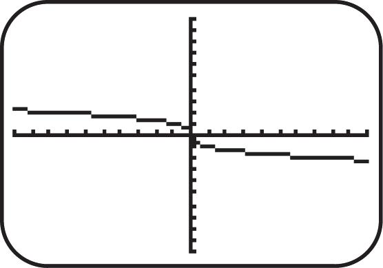
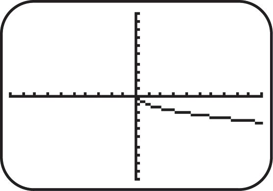
Figure 28 Figure 29 Figure 30
31. Graph 3 ()1.fxx See Figure 31. As x increases for the interval (,), y decreases; therefore, the function is decreasing.
32. Graph 2 ()2. fxxx See Figure 32. As x increases for the interval 1, y increases; therefore, the function is increasing on 1, .
33. Graph 2 ()2.fxx See Figure 33. As x increases for the interval ,0 y increases; therefore, the function is increasing on ,0
34. Graph ()|1|.fxx See Figure 34. As x increases for the interval ,1 y decreases; therefore, the function is decreasing on ,1 . [-10,10] by [-10,10] [-10,10] by [-10,10] [-10,10] by [-10,10] [-10,10] by [-10,10]
Xscl = 1 Yscl = 1 Xscl = 1 Yscl = 1 Xscl= 1 Yscl = 1 Xscl = 1 Yscl= 1
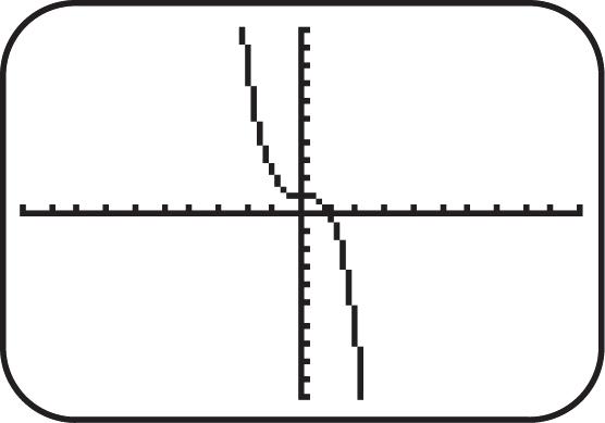
Figure 31

Figure 32
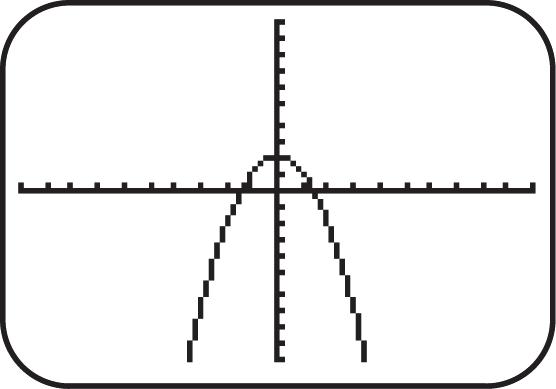
Figure 33
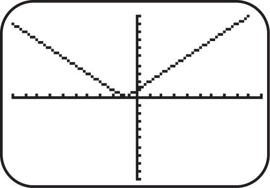
Figure 34
35. (a) No (b) Yes (c) No
36. (a) Yes (b) No (c) No
37. (a) Yes (b) No (c) No
38. (a) No (b) No (c) Yes
39. (a) Yes (b) Yes (c) Yes
40. (a) Yes (b) Yes (c) Yes
41. (a) No (b) No (c) Yes
42. (a) No (b) Yes (c) No
43. Since the graph is symmetric with respect to the y-axis the function is even.
44. Since the graph is symmetric with respect to the origin the function is odd.
45. Since the graph is symmetric with respect to the origin the function is odd.
46. Since the graph is symmetric with respect to the y-axis the function is even.
47. Since the graph is not symmetric with respect to the y-axis or orign, the function is neither even nor odd.
48. Since the graph is not symmetric with respect to the y-axis or orign, the function is neither even nor odd.
49. (a) Since ()(),fxfx this is an even function and is symmetric with respect to the y-axis.
See Figure 49a. (b) Since ()(), fxfx this is an odd function and is symmetric with respect to the origin.
See Figure 49b.

Figure 49a
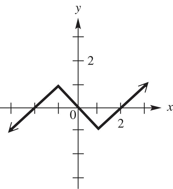
Figure 49b
50. (a) Since this is an odd function and is symmetric with respect to the origin. See Figure 50a. (b) Since this is an even function and is symmetric with respect to the y-axis. See Figure 50b

Figure 50a
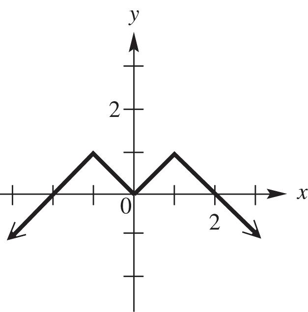
Figure 50b
51. If f is an even function then ()() fxfx or opposite domains have the same range. See Figure 51
52. If g is an odd function then ()() gxgx or opposite domains have the opposite range. See Figure 52
Copyright © 2019 Pearson Education, Inc.
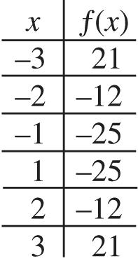
Figure 51

Figure 52
53. This is an even function since opposite domains have the same range.
54. This is an even function since opposite domains have the same range.
55. This is an odd function since opposite domains have the opposite range.
56. This is an odd function since opposite domains have the opposite range.
57. This is neither even nor odd since the opposite domains are neither the opposite or same range.
58. This is neither even nor odd since the opposite domains are neither the opposite or same range.
59. If 42 ()76, fxxx then 4242 ()()7()6()76. fxxxfxxx
Since ()(),fxfx the function is even.
60. If 62 ()28, fxxx then 6262 ()2()8()()28. fxxxfxxx
Since ()(),fxfx the function is even.
61. If 3 ()3, fxxx then 33 ()3()()()3 fxxxfxxx
and 33 ()(3)()3. fxxxfxxx Since ()(), fxfx the function is odd.
62. If 53 ()23, fxxxx then 5353 ()()2()3()()23 fxxxxfxxxx and 5353 ()(23)()23. fxxxxfxxxx Since ()(), fxfx the function is odd.
63. If 64 ()45 fxxx then 6464 ()()4()5()45. fxxxfxxx Since ()(),fxfx the function is even.
64. If ()8,fx then ()8.fx Since ()(),fxfx the function is even.
65. If 53 ()37, fxxxx then 5353 ()3()()7()()37 fxxxxfxxxx and 5353 ()(37)()37. fxxxxfxxxx Since ()(), fxfx the function is odd.
66. If 3 ()4, fxxx then 33 ()()4()()4 fxxxfxxx
and 33 ()(4)()4. fxxxfxxx
Since ()(), fxfx the function is odd.
67. If ()|5|,fxx then ()|5()|()|5|. fxxfxx
Since ()(),fxfx the function is even.
68. If 2 ()1,fxx then 22 ()()1()1. fxxfxx Since ()(),fxfx the function is even.
81. If 3 ()3,fxxx then 33 ()()()3()3 fxxxfxxx and 33 ()(3)()3. fxxxfxxx Since ()()(), fxfxfx the function is not symmetric with respect to the y-axis or the origin.
82. If 4 ()52, fxxx then 44 ()()5()2()52 fxxxfxxx and 44 ()(52)()52. fxxxfxxx Since ()()(), fxfxfx the function is not symmetric with respect to the y-axis or the origin. Graph 4 ()52; fxxx the graph supports no symmetry with respect to the y-axis or the origin.
83. If 63 ()4, fxxx then 6363 ()()4()()4 fxxxfxxx and 6363 ()(4)()4. fxxxfxxx
Since ()()(), fxfxfx the function is not symmetric with respect to the y-axis or the origin. Graph 63 ()4; fxxx the graph supports no symmetry with respect to the y-axis or the origin.
84. If 3 ()3, fxxx then 33 ()()3()()3 fxxxfxxx and 33 ()(3)()3. fxxxfxxx Since ()(), fxfx the function is symmetric with respect to the origin. Graph 3 ()3; fxxx the graph supports symmetry with respect to the origin.
85. If ()6,fx then ()6,fx Since ()(),fxfx the function is symmetric with respect to the yaxis. Graph ()6;fx the graph supports symmetry with respect to the y-axis.
86. If ()||,fxx then ()|()|()||. fxxfxx Since ()(),fxfx the function is symmetric with respect to the y-axis. Graph ()||;fxx the graph supports symmetry with respect to the y-axis.
87. If 3 1 (), 4 fx x then 33 11 ()()4()4 fxfx xx
and 33 11 ()(). 44fxfx xx
Since ()(), fxfx the function is symmetric with respect to the origin. Graph 3 1 (); 4 fx x the graph supports symmetry with respect to the origin.
88. If 2 ()(), fxxfxx then 22 ()()()(). fxxfxxfxx
Since ()(),fxfx the function is symmetric with respect to the y-axis. Graph 2 ();fxx the graph
2.2: Vertical and Horizontal Shifts of Graphs
1. The equation 2 yx shifted 3 units upward is 2 3. yx
2. The equation 3 yx shifted 2 units downward is 3 2. yx
3. The equation yx shifted 4 units downward is 4. yx
4. The equation 3 yx shifted 6 units upward is 3 6. yx
Copyright © 2019 Pearson Education, Inc.
5. The equation ||yx shifted 4 units to the right is |4|.yx
6. The equation ||yx shifted 3 units to the left is |3|.yx
7. The equation 3 yx shifted 7 units to the left is 3 (7).yx
8. The equation yx shifted 9 units to the right is 9. yx
9. The equation 2 yx shifted 2 units downward and 3 units right is 2 32. yx
10. The equation 2 yx shifted 4 units upward and 1 unit left is 2 14. yx
11. The equation yx shifted 3 units upward and 6 units to the left is 63. yx
12. The equation ||yx shifted 1 unit downward and 5 units to the right is |5|1.yx
13. The equation 2 yx shifted 500 units upward and 2000 units right is 2 2000500. yx
14. The equation 2 yx shifted 255 units downward and 1000 units left is 2 1000255. yx
15. Shift the graph of f 4 units upward to obtain the graph of g.
16. Shift the graph of f 4 units to the left to obtain the graph of g.
17. The equation 2 3 yx is 2 yx shifted 3 units downward; therefore, graph B.
18. The equation 2 (3)yx is 2 yx shifted 3 units to the right; therefore, graph C.
19. The equation (3)2yx is 2 yx shifted 3 units to the left; therefore, graph A.
20. The equation || 4 yx is ||yx shifted 4 units upward; therefore; graph A.
21. The equation |4| 3 yx is ||yx shifted 4 units to the left and 3 units downward; therefore, graph B.
22. The equation |4| 3 yx is ()yfx shifted 4 units to the right and 3 units downward; therefore, graph C.
23. The equation (3)3yx is 3 yx shifted 3 units to the right; therefore, graph C.
24. The equation 3 (2)4yx is 3 yx shifted 2 units to the right and 4 units downward; therefore, graph A.
25. The equation 3 (2)4yx is ,.ab shifted 2 units to the left and 4 units downward; therefore, graph B.
26. Using 21 YYk and 0. x we get 19154. kk
27. Using 21 YYk and 0, x we get 532. kk
28. Using 21 YYk and 0 x , we get 5.541.51.5. k
29. From the graphs, (6,2) is a point on 1Y and (6,1) a point on 2Y Using 21 YYk and 6, x we get 123. kk
30. From the graphs, (4,3) is a point on 1Y and (4,8) a point on 2Y Using 21 YYk and4, x we get 835. kk
Copyright © 2019 Pearson Education, Inc.
31. For the equation 2 , yx the Domain is (,) and the Range is [0,). Shifting this 3 units downward gives us: (a) Domain: (,) (b) Range: [3,).
32. For the equation 2 , yx the Domain is (,) and the Range is [0,). Shifting this 3 units to the right gives us: (a) Domain: (,) (b) Range: [0,) .
33. For the equation ||,yx the Domain is (,) and the Range is [0,). Shifting this 4 units to the left and 3 units downward gives us: (a) Domain: (,) (b) Range: [3,)
34. For the equation ||,yx the Domain is (,) and the Range is [0,). Shifting this 4 units to the right and 3 units downward gives us: (a) Domain: (,) (b) Range: [3,).
35. For the equation 3 , yx the Domain is (,) and the Range is (,). Shifting this 3 units to the right gives us: (a) Domain: (,) (b) Range: (,)
36. For the equation 3 , yx the Domain is (,) and the Range is (,) . Shifting this 2 units to the right and 4 units downward gives us: (a) Domain: (,) (b) Range: (,)
37. For the equation 2 , yx the Domain is (,) and the Range is [0,). Shifting this 1 unit to the right and 5 units downward gives us: (a) Domain: (,) (b) Range: [5,)
38. For the equation 2 , yx the Domain is (,) and the Range is [0,). Shifting this 8 units to the left and 3 units upward gives us: (a) Domain: (,) (b) Range: [3,)
39. For the equation , yx the Domain is [0,). and the Range is [0,). Shifting this 4 units to the right gives us: (a) Domain: [4,). (b) Range: [0,)
40. For the equation , yx the Domain is [0,). and the Range is [0,). Shifting this 1 units to the left and 10 units downward gives us: (a) Domain: [1,). (b) Range: [10,)
41. For the equation 3 , yx the Domain is (,) and the Range is (,) . Shifting this 1 unit to the right and 4 units upward gives us: (a) Domain: (,) (b) Range: (,)
42. For the equation 3 , yx the Domain is (,) and the Range is (,) . Shifting this 7 units to the left and 10 units downward gives us: (a) Domain: (,) (b) Range: (,)
43. The graph of ()yfx is the graph of the equation 2 yx shifted 1 unit to the right. See Figure 43.
44. The graph of 2 yx is the graph of the equation yx shifted 2 units to the left. See Figure 44.
45. The graph of 3 1 yx is the graph of the equation 3 yx shifted 1 unit upward. See Figure 45.

Figure 43
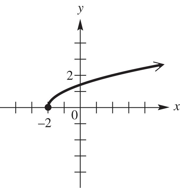
Figure 44

Figure 45
46. The graph of |2|yx is the graph of the equation ||yx shifted 2 units to the left. See Figure 46.
47. The graph of (1)3yx is the graph of the equation 3 yx shifted 1 unit to the right. See Figure 47.
48. The graph of || 3 yx is the graph of the equation ||yx shifted 3 units downward. See Figure 48.
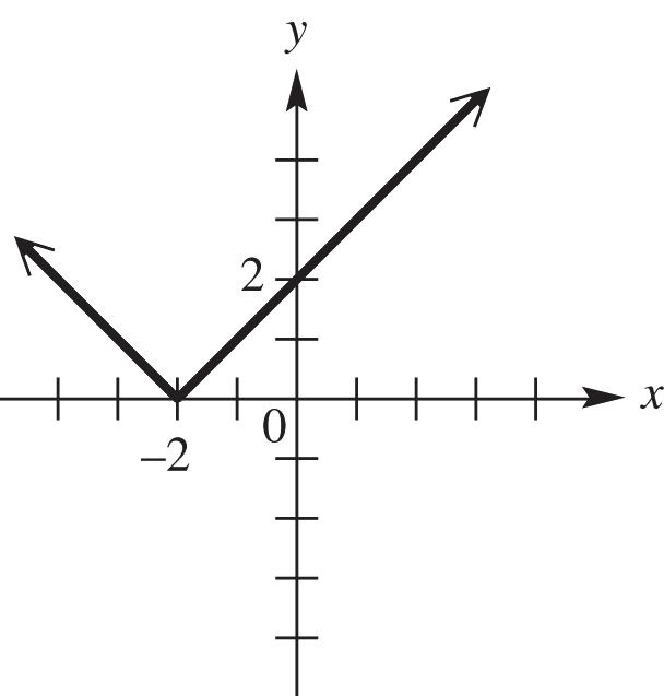
Figure 46

Figure 47
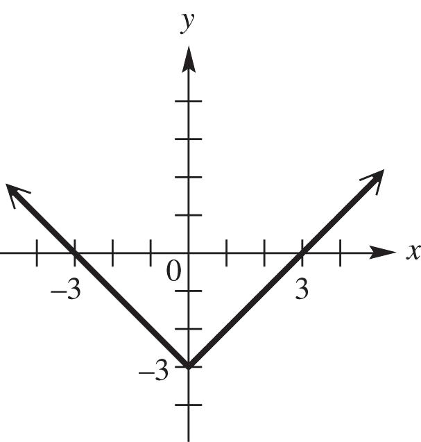
Figure 48
49. The graph of 2 1 yx is the graph of the equation yx shifted 2 units to the right and 1 unit downward. See Figure 49.
50. The graph of 3 4 yx is the graph of the equation yx shifted 3 units to the left and 4 units downward. See Figure 50.
51. The graph of ()fx is the graph of the equation 2 yx shifted 2 units to the left and 3 units upward. See Figure 51.

Figure 49
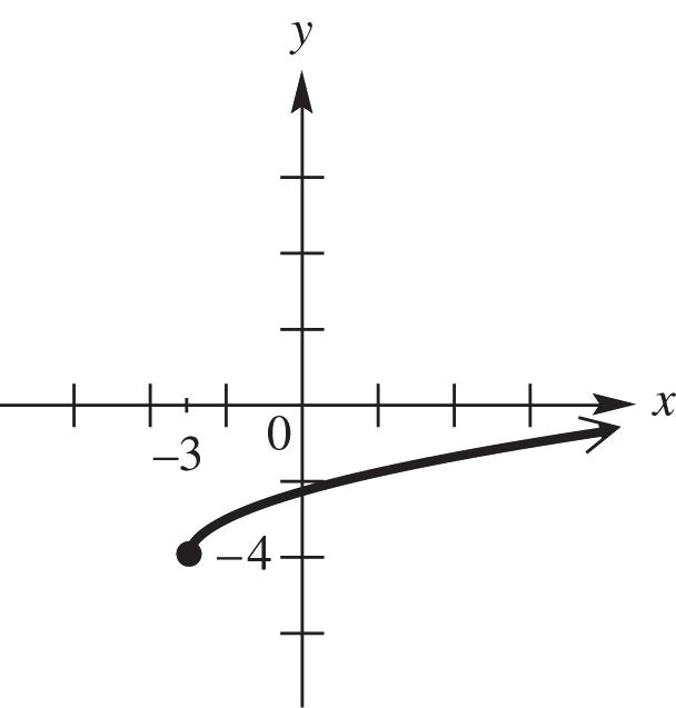
Figure 50

Figure 51
52. The graph of (4)2 4 yx is the graph of the equation 2 yx shifted 4 units to the right and 4 units downward. See Figure 52.
53. The graph of |4| 2 yx is the graph of the equation ||yx shifted 4 units to the left and 2 units downward. See Figure 53.
54. The graph of (3)3 1 yx is the graph of the equation 3 yx shifted 3 units to the left and 1 unit downward. See Figure 54.
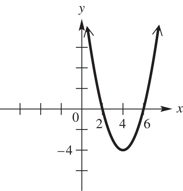
Figure 52

Figure 53
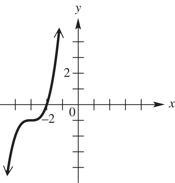
Figure 54
55. Since h and k are positive, the equation is 2 yx shifted to the right and down; therefore, B.
56. Since h and k are positive, the equation is 2 yx shifted to the left and down; therefore, D.
57. Since h and k are positive, the equation is 2 yx shifted to the left and up; therefore, A.
58. Since h and k are positive, the equation is 2 yx shifted to the right and up; therefore, C.
59. The equation ()2yfx is ()yfx shifted up 2 units or add 2 to the y-coordinate of each point as follows: (3,2)(3,0);(1,4)(1,6);(5,0)(5,2). See Figure 59.
60. The equation ()2yfx is ()yfx shifted down 2 units or subtract 2 from the y-coordinate of each point as follows: (3,2)(3,4);(1,4)(1,2);(5,0)(5,2). See Figure 60.
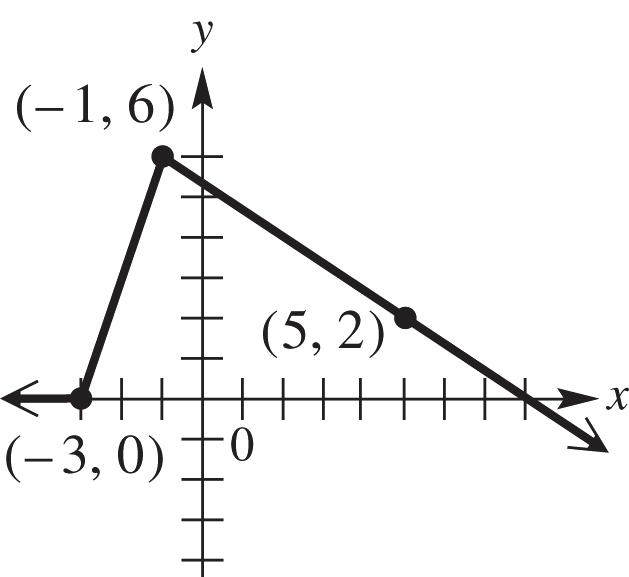
Figure 59
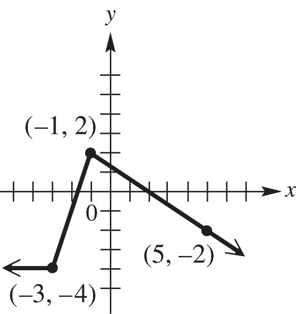
Figure 60
61. The equation (2)yfx is ()yfx shifted left 2 units or subtract 2 from the x-coordinate of each point as follows: (3,2)(5,2);(1,4)(3,4);(5,0)(3,0). See Figure 61.
62. The equation (2)yfx is ()yfx shifted right 2 units or add 2 to the x-coordinate of each point as follows: (3,2)(1,2);(1,4)(1,4);(5,0)(7,0). See Figure 62.

Figure 61

Figure 62
Copyright © 2019 Pearson Education, Inc.
63. The graph is the basic function 2 yx translated 4 units to the left and 3 units up; therefore, the new equation is 2 (4)3.yx The equation is now increasing for the interval: (a) 4, and decreasing for the interval: (b) ,4 .
64. The graph is the basic function yx translated 5 units to the left; therefore, the new equation is 5. yx
The equation is now increasing for the interval: (a) 5, and does not decrease; therefore: (b) none.
65. The graph is the basic function 3 yx translated 5 units down; therefore, the new equation is 3 5. yx
The equation is now increasing for the interval: (a) (,) and does not decrease; therefore: (b) none.
66. The graph is the basic function ||yx translated 10 units to the left; therefore, the new equation is | 10|. yx The equation is now increasing for the interval: (a) 10, and decreasing for the interval: (b) ,10
67. The graph is the basic function yx translated 2 units to the right and 1 unit up; therefore, the new equation is 2 1. yx The equation is now increasing for the interval: (a) 2, and does not decrease; therefore: (b) none.
68. The graph is the basic function 2 yx translated 2 units to the right and 3 units down; therefore, the new equation is 2 (2)3.yx The equation is now increasing for the interval: (a) 2, and decreasing for the interval: (b) ,2 .
69. The translation is 3 units to the left and 1 unit up; therefore, the new equation is |3| 1. yx The form || yxhk will equal |3| 1 yx when: 3 h and 1. k
70. The equation 2 yx has a Domain: (,) and a Range: [0,). After the translation the Domain is still: (,) but now the Range is (38,) , a positive or upward shift of 38 units. Therefore, the horizontal shift can be any number of units, but the vertical shift is up 38. This makes h any real number and 38. k
71. (a) O(9)2649.4(9)13,26037,104.6 ; In 2014, organic food sales totaled $37,104.6 million.
(b) We will use the point (2005, 13260) and the slope of 2649.4 in the point slope form for the equation of a line. 11()136202649.4(2005)2649.4(2005)13620 yymxxyxyx (c) 2649.4(20142005)1362037,104.6 y (d) 12,887 26,5072649.4(2005)1362012,8872649.4(2005)20052009.86 2649.4 xxxx
The organic food sales reached $26,507 around 2010.
72. (a) (3)23.8(3)248176.6 S ; In 2013, 176.6 million units were sold.
Copyright © 2019 Pearson Education, Inc.
(b) We will use the point (2010, 248) and the slope of 23.8 in the point slope form for the equation of a line. 11()24823.8(2010)23.8(2010)248 yymxxyxyx
(c) 23.8(20132010)24823.8(3)248176.6 y ; In 2013, 176.6 million units were sold.
(d) 12923.8(2010)24811923.8(2010)520102015 xxxx
73. 2 (2011)13(20112006)11513(25)115440 U ; The average U.S. household spent $440 on Apple products in 2011.
74. The formula for ()Wx can be found by shifting 2 ()13(2006)115Uxx to the right 4 units. 2 ()13(2010)115Wxx ; 2 ()13(20152010)11513(25)115440Wx
In 2015, the average worldwide household spending on Apple products was $440, which equaled U.S. spending 4 years earlier.
75. (a) Enter the year in 1L and enter tuition and fees in 2L . The year 2000 corresponds to 0 x and so on. The regression equation is 397.23526.yx
(b) Since 0 x corresponds to 2000, the equation when the exact year is entered is 397.2(2000)3526yx
(c) 397.2(20142000)35269087 y
76. (a) Enter the year in 1L and enter the percent of women in the workforce in 2L The year 2015 corresponds to 0 x and so on. The regression equation is 404.129136.25.yx
(b) Since 0 x corresponds to 2015, the equation when the exact year is entered is 404.1220159136.25.yx
(c) 404.12202520159136.2513,177. y
77. See Figure 77.
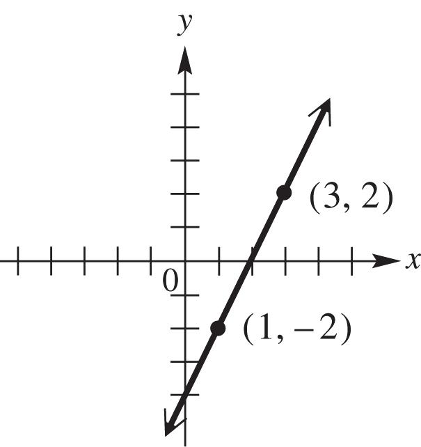
Figure 77
78. 2(2)4 2 312 mm
79. Using slope-intercept form yields: 111 22(3)22624 yxyxyx
Copyright © 2019 Pearson Education, Inc.
80. (1,26) and (3,26)(1,4) and (3,8)
81. 844 2 312 mm
82. Using slope-intercept form yields: 222 42(1)42222 yxyxyx .
83. Graph 1 24yx and 2 22yx See Figure 87. The graph 2y can be obtained by shifting the graph of 1y upward 6 units. The constant 6, comes from the 6 we added to each y-value in Exercise 84. [-10,10] by [-10,10] Xscl = 1 Yscl = 1
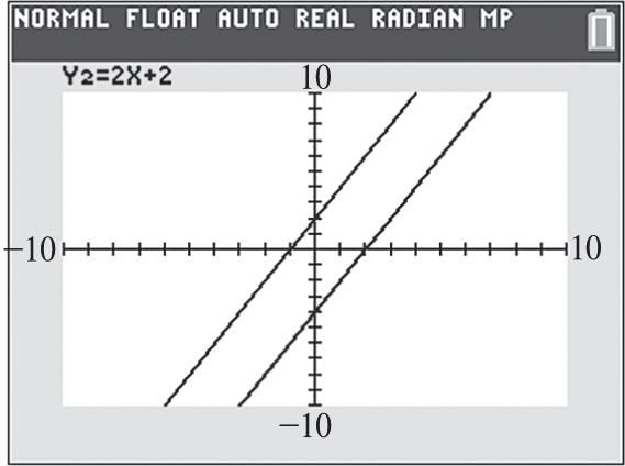
Figure 83
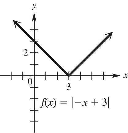
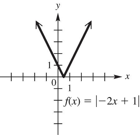
84. c; c; the same as; c; upward (or positive vertical)
2.3: Stretching, Shrinking, and Reflecting Graphs
1. The function 2 yx vertically stretched by a factor of 2 is 2 2.yx
2. The function 3 yx vertically shrunk by a factor of one half is 3 1 2 yx
3. The function yx reflected across the y-axis is yx
4. The function 3 yx reflected across the x-axis is 3 yx
5. The function yx vertically stretched by a factor of 3 and reflected across the x-axis is 3.yx
6. The function yx vertically shrunk by a factor of one-half and reflected across the y-axis is 1 . 3 yx
7. The function 3 yx vertically shrunk by a factor of 0.25 and reflected across the y-axis is 3 0.25()yx or 3 0.25.yx
8. The function yx vertically shrunk by a factor of 0.2 and reflected across the x-axis is 0.2 yx
9. Graph 1 yx , 2 3 yx ( 1y shifted up 3 units), and 3 3 yx ( 1y shifted down 3 units). See Figure 9.
10. Graph 3 1 yx , 3 2 4 yx ( 1y shifted up 4 units), and 3 3 4 yx ( 1y shifted down units).
See Figure 10.
11. Graph 1 yx , 2 3 yx ( 1y shifted right 3 units), and 3 3 yx ( 1y shifted left 3 units). See Figure 11.
Copyright © 2019 Pearson Education, Inc.
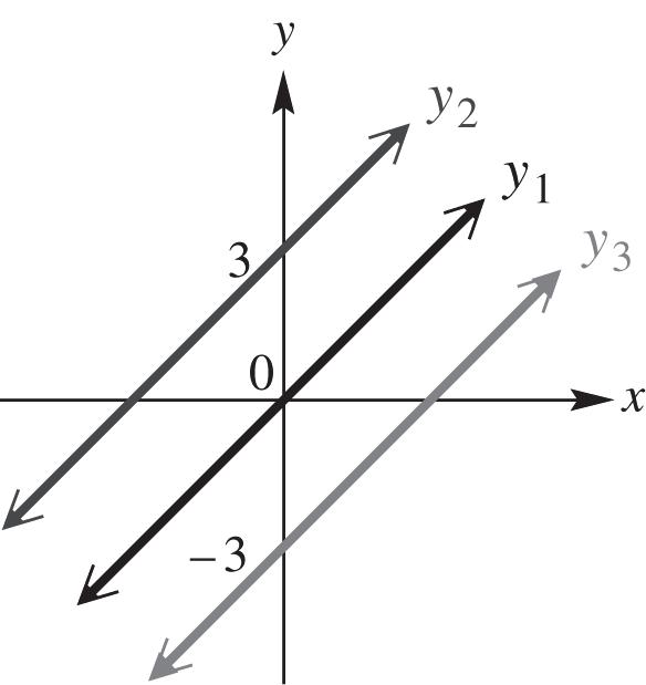
Figure 9
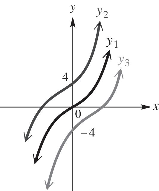
Figure 10
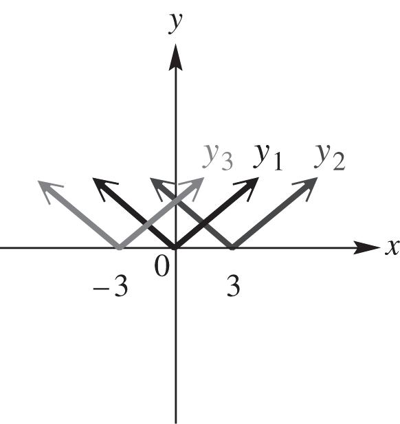
Figure 11
12. Graph 1 , yx 2 3 yx ( 1y shifted down 3 units), and 3 3 yx ( 1y shifted up 3 units).
See Figure 12.
13. Graph 1 , yx 2 6 yx ( 1y shifted left 6 units), and 3 6 yx ( 1y shifted right 6 units). See Figure 13.
14. Graph 1 yx , 2 2 yx ( 1y stretched vertically by a factor of 2), and 3 2.5 yx ( 1y stretched vertically by a factor of 2.5). See Figure 14
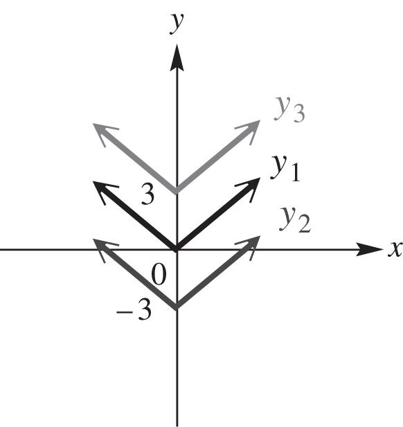
Figure 12

Figure 13
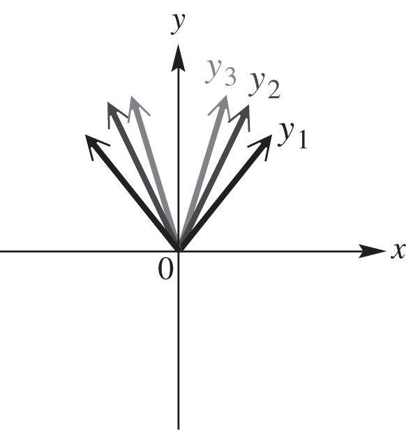
Figure 14
15. Graph 3 1 , yx 3 2 yx ( 1y reflected across the x-axis), and 3 3 2 yx ( 1y reflected across the x-axis and stretched vertically by a factor of 2). See Figure 15
16. Graph 2 1 , yx 2 2 (2) 1 yx ( 1y shifted right 2 units and up 1 unit), and 2 3 (2)yx ( 1y shifted left 2 units and reflected across the x-axis). See Figure 16
17. Graph 1 , yx 2 211yx ( 1y reflected across the x-axis, stretched vertically by a factor of 2, shifted right 1 unit, and shifted up 1 unit), and 3 1 4 2 yx ( 1y reflected across the x-axis, shrunk by factor of 1 , 2 and shifted down 4 units). See Figure 17

Figure 15
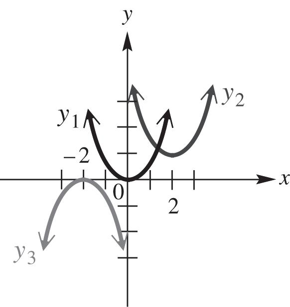
Figure 16

17
18. Graph 1 , yx 2 yx ( 1y reflected across the x-axis), and 3 yx ( 1y reflected across the y-axis). See Figure 18.
19. Graph 2 1 1 yx (which is 2 yx shifted down 1 unit),
( 1y shrunk vertically by A factor of 1 2 ), and 2 3 21yx ( 1y stretched vertically by a factor of 22 or 4). See Figure 19.
20. Graph 1 3 yx (which is yx reflected across the x-axis and shifted up 3 units), 2 33 yx stretched vertically by a factor of 3), and 3 1 3 3 yx ( 1y shrunk vertically by a factor of 1 3 ). See Figure 20
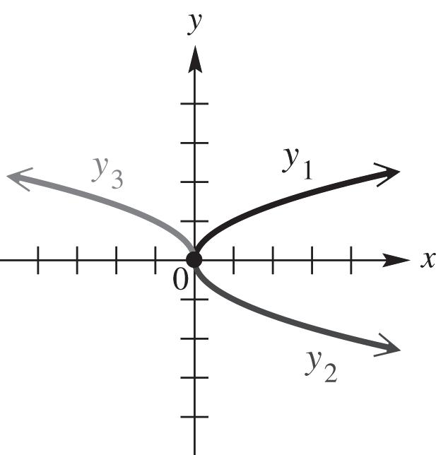
Figure 18
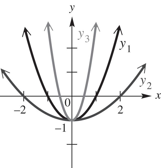
Figure 19

Figure 20
21. Graph 3 1 , yx 3 2 yx ( 1y reflected across the y-axis), and 3 3 (1)yx ( 1y reflected across the y-axis and shifted right 1 unit). See Figure 21.
22. Graph 3 1 , yx 3 2 2 yx ( 1y reflected across the x-axis and shifted up 2 units), and 3 3 1 yx ( 1y shifted up 1 unit). See Figure 22.
Copyright © 2019 Pearson Education, Inc.
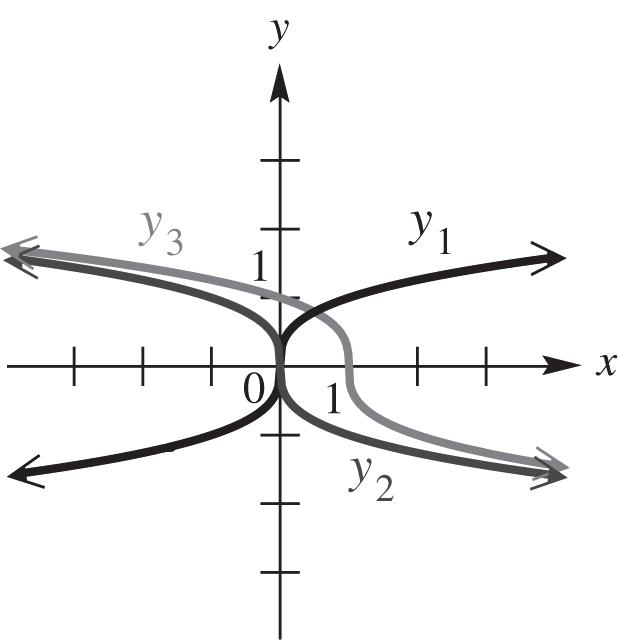
21

22
23. The graph 2 () yfxx has been reflected across the x-axis, shifted 5 units to the right, and shifted 2 units downward; therefore, the equation of ()gx is 2 ()(5)2.gxx
24. The graph 3 () yfxx has been shifted 4 units to the right and shifted 3 units upward; therefore, the equation of ()gx is 3 ()(4)3gxx .
25. The graph () yfxx has been reflected across the y-axis and shifted 1 unit upward; therefore, the equation of ()gx is ()1gxx
26. The graph 3 () yfxx has been reflected across the x-axis and shifted 2 units to the right; therefore, the equation of ()gx is 3 ()2gxx .
27. 4; x
28. 6; x
29. 2; left; 1 ; 4 ; 3; x downward (or negative)
30. 2 ; ; ; 6 5 yx upward (or positive)
31. 3; right; 6
32. 2; left; 0.5
33. The function 2 yx is vertically shrunk by a factor of 1 2 and shifted 7 units down; therefore, 2 1 7 2 yx .
34. The function 3 yx is vertically stretched by a factor of 3 , reflected across the x-axis, and shifted 8 units upward; therefore, 38yx .
35. The function yx is shifted 3 units right, vertically stretched by a factor of 4.5, and shifted 6 units down; therefore, 4.536.yx
36. The function 3 yx is shifted 2 units left, vertically stretched by a factor of 1.5 , and shifted 8 units upward; therefore, 3 1.528.yx
37. The function ()32fxx is () fxx shifted 3 units right and 2 units upward. See Figure 37.
38. The function ()23fxx is () fxx shifted 2 units left and 3 units downward. See Figure 38.
39. The function ()22 fxxx is () fxx stretched vertically by a factor of 2 . See Figure 39.
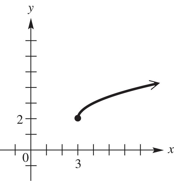
Figure 37
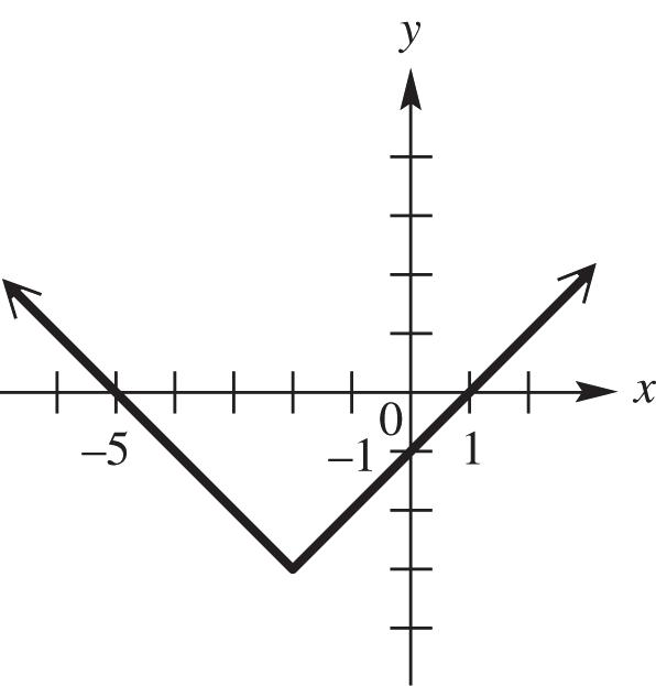
Figure 38

Figure 39
40. The function 2 1 ()(2) 2 fxx is 2 () fxx shifted 2 units left and shrunk vertically by a factor of 1 2
See Figure 40.
41. The function ()22 fxxx is () fxx stretched vertically by a factor of 2. See Figure 41.
42. The function 1 () 2 fxx is () fxx shrunk vertically by a factor of 1 2 . See Figure 42

Figure 40
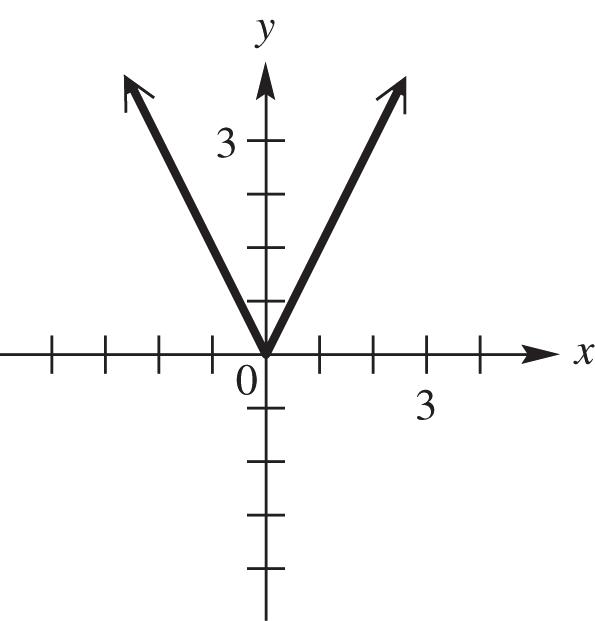
Figure 41

Figure 42
43. The function ()1 fxx is () fxx reflected across the x-axis and shifted 1 unit upward. See Figure 43.
44. The function ()221fxx is () fxx shifted 2 units right, stretched vertically by a factor of 2, and shifted 1 unit downward. See Figure 44.
45. The function ()1(1) fxxx is () fxx reflected across both the x-axis, the y-axis and shifted 1 unit right. See Figure 45.

Figure 43
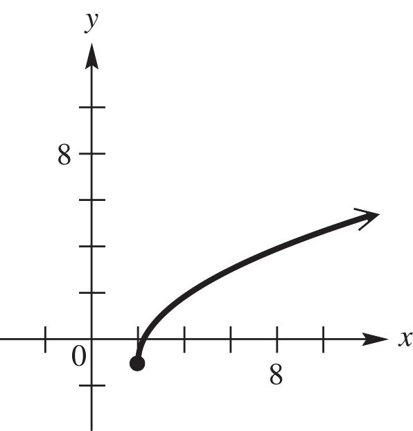
Figure 44
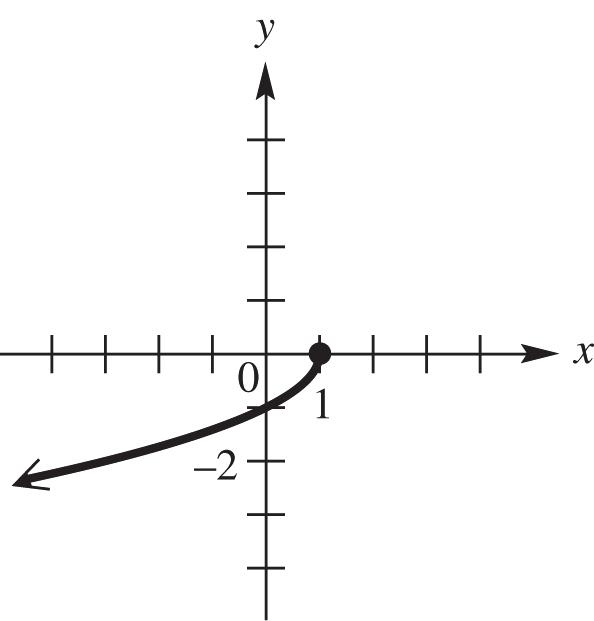
Figure 45
46. The function ()1fxx is () fxx reflected across the y-axis and shifted 1 unit downward.
See Figure 46.
47. The function ()(1)fxx is () fxx reflected across the y-axis and shifted 1 unit left. See Figure 47.
48. The function ()2(3) fxx is () fxx reflected across the y-axis, shifted 3 units right, and shifted 2 units upward. See Figure 48.
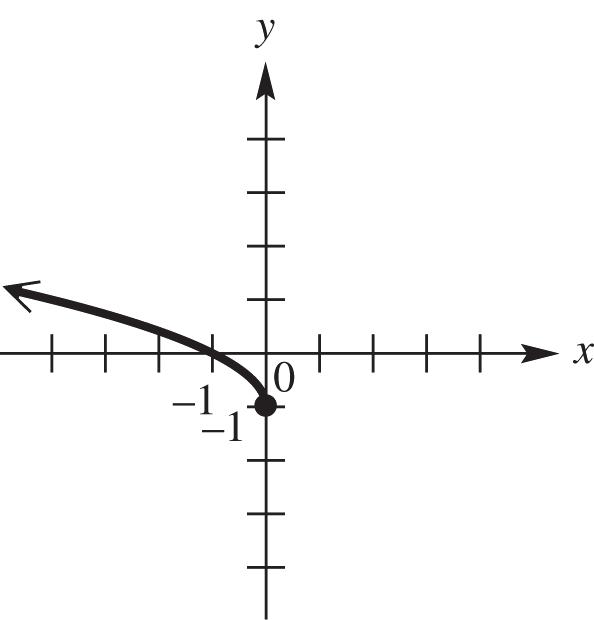
Figure 46
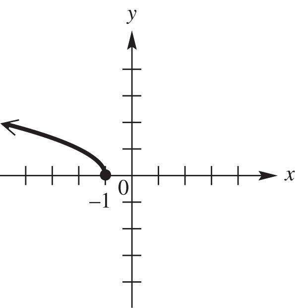
Figure 47
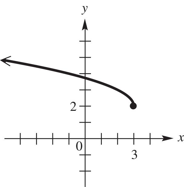
Figure 48
49. The function ()(1)3fxx is 3 () fxx shifted 1 unit right. See Figure 49.
50. The function ()(2)3fxx is 3 () fxx shifted 2 unit left. See Figure 50.
51. The function 3 () fxx is 3 () fxx reflected across the x-axis. See Figure 51.
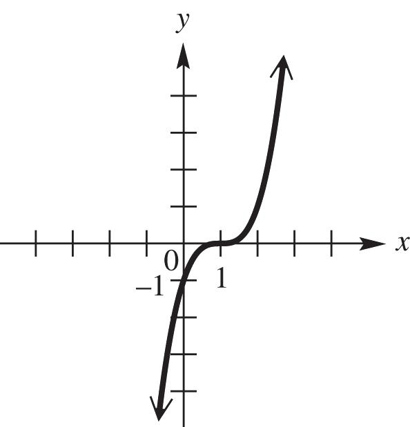
Figure 49
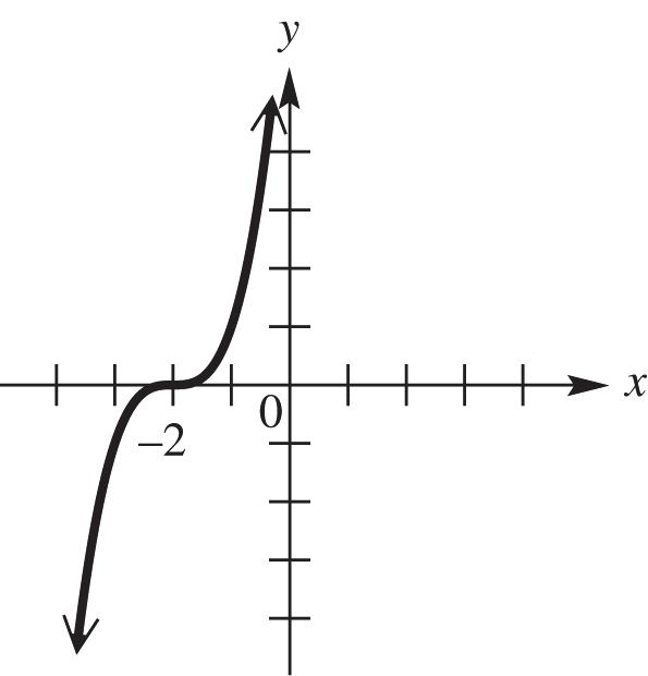
Figure 50
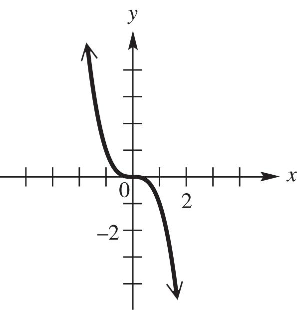
Figure 51
52. The function 3 ()()1fxx is 3 () fxx reflected across the y-axis and shifted 1 unit upward. See Figure 52.

Figure 52
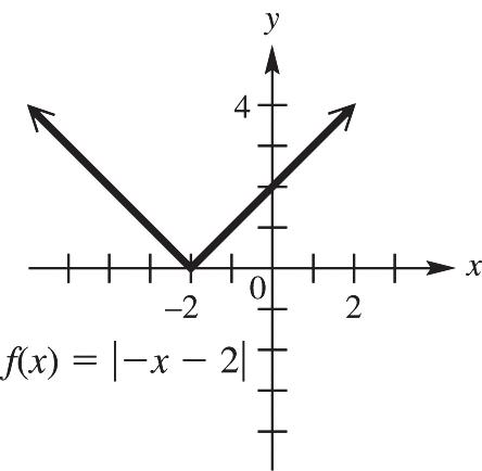
Figure 53
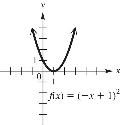
Figure 54
53. The function ()2fxx is () fxx shifted two units to the right and reflected across the y-axis. See Figure 53.
54. The function ()(1)2fxx is 2 () fxx shifted one unit to the left and reflected across the y-axis. See Figure 54.
55. The function ()3fxx is () fxx shifted three units to the left and reflected across the y-axis. See Figure 55.
56. The function ()21fxx is () fxx stretched vertically by a factor of 2, shifted one units to the left and reflected across the y-axis. See Figure 56.
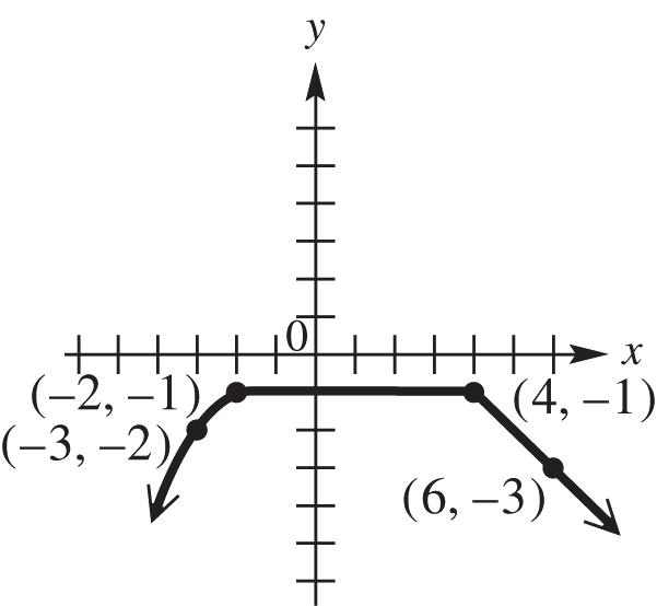
56
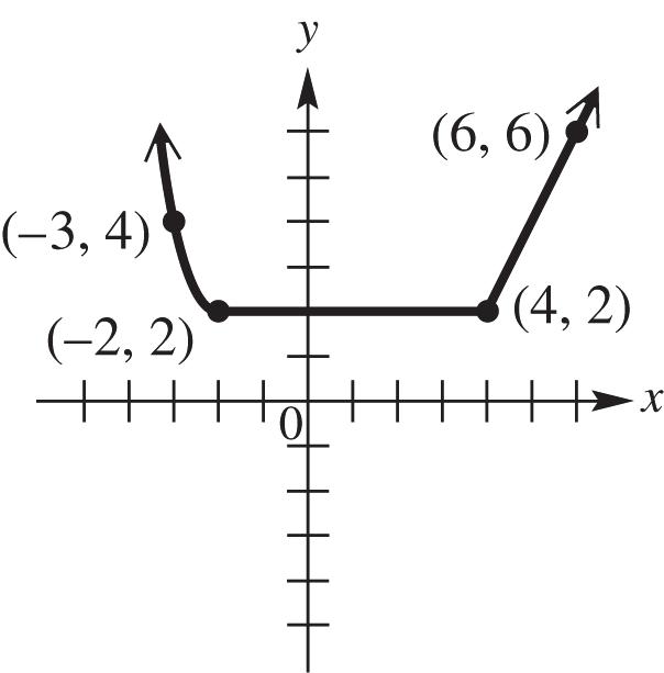
57. (a) The equation ()yfx is ()yfx reflected across the x-axis. See Figure 57a.
(b) The equation ()yfx is ()yfx reflected across the y-axis. See Figure 57b.
(c) The equation 2()yfx is ()yfx stretched vertically by a factor of 2. See Figure 57c.
(d) From the graph (0)1. f
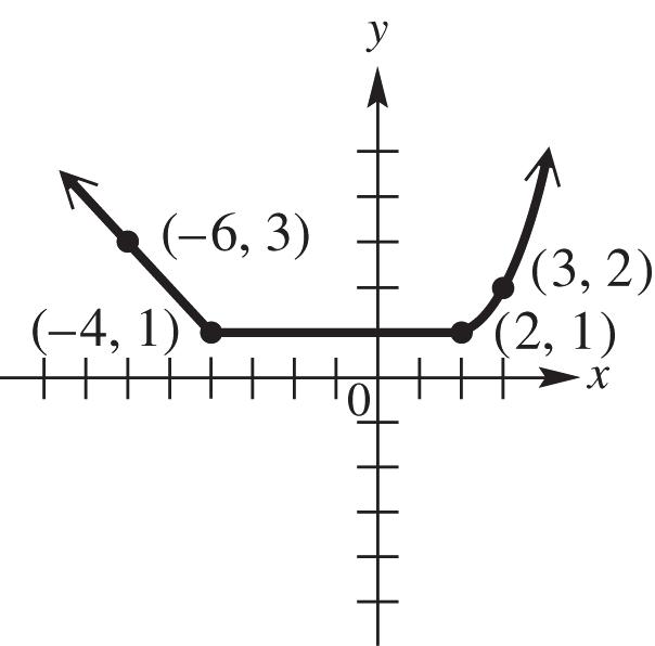
58. (a) The equation ()yfx is ()yfx reflected across the x-axis. See Figure 58a.
(b) The equation ()yfx is ()yfx reflected across the y-axis. See Figure 58b.
(c) The equation 3()yfx is ()yfx stretched vertically by a factor of 3. See Figure 58c.
(d) From the graph (4)1 f

Figure 58a
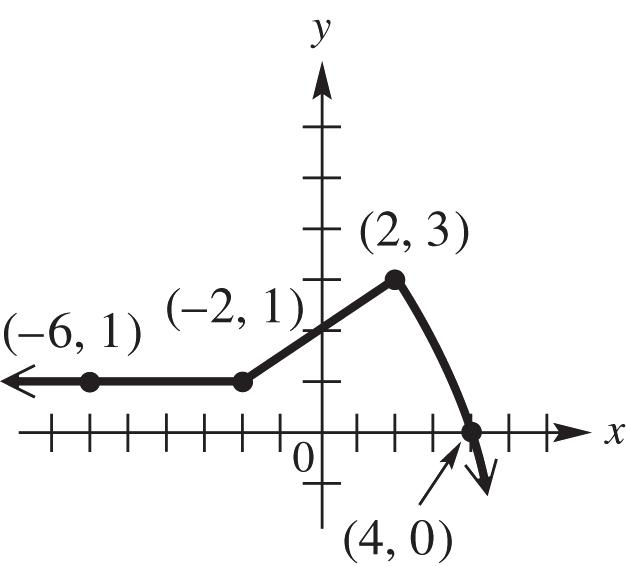
Figure 58b
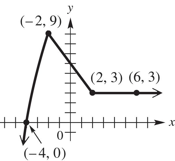
Figure 58c
Copyright © 2019 Pearson Education, Inc.
59. (a) The equation ()fx is ()yfx reflected across the x-axis. See Figure 59a.
(b) The equation ()yfx is ()yfx reflected across the y-axis. See Figure 59b.
(c) The equation (1)yfx is ()yfx shifted 1 unit to the left. See Figure 59c.
(d) From the graph, there are two x-intercepts, 1,0 and 4,0
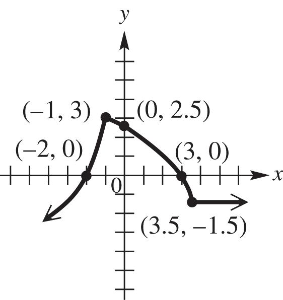
Figure 59a
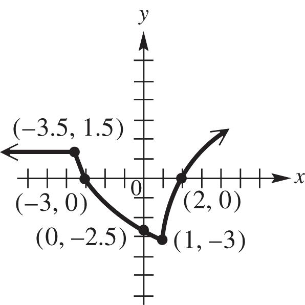
Figure 59b

Figure 59c
60. (a) The equation ()yfx is ()yfx reflected across the x-axis. See Figure 60a.
(b) The equation ()yfx is ()yfx reflected across the y-axis. See Figure 60b.
(c) The equation 1 () 2 yfx is 20,5. shrunk vertically by a factor of 1 . 2 See Figure 60c.
(d) From the graph ()0fx for the interval: ,0.
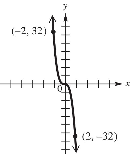
Figure 60a

Figure 60b

Figure 60c
61. (a) The equation ()yfx is ()yfx reflected across the x-axis. See Figure 61a.
(b) The equation 1 3 yfx
is ()yfx stretched horizontally by a factor of 3. See Figure 61b.
(c) The equation 0.5()yfx is ()yfx shrunk vertically by a factor of 0.5. See Figure 61c.
(d) From the graph, symmetry with respect to the origin.
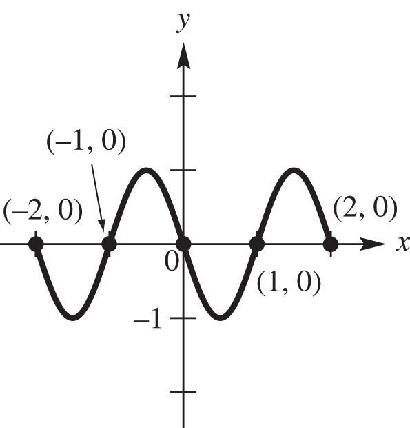
Figure 61a
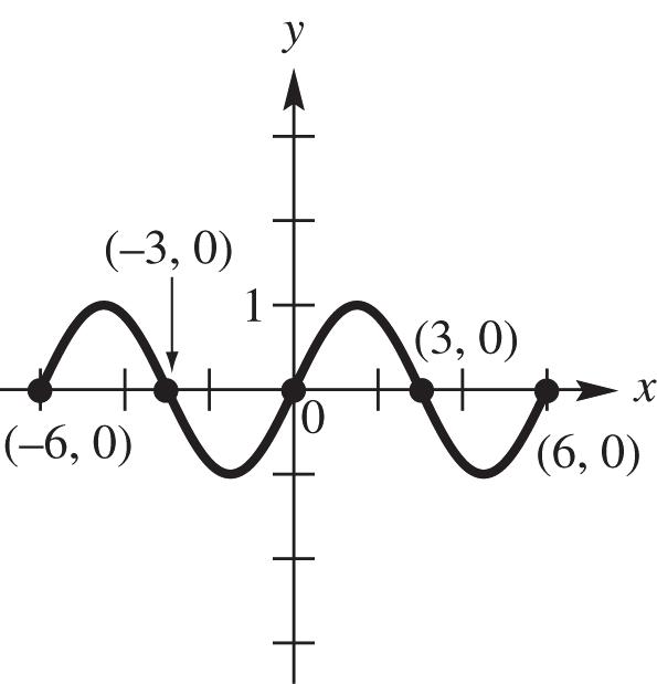
Figure 61b

Figure 61c
62. (a) The equation (2)yfx is ()yfx stretched horizontally by a factor of 1 2 See Figure 62a
(b) The equation ()yfx is ()yfx reflected across the y-axis. See Figure 62b.
(c) The equation 3()yfx is ()yfx stretched vertically by a factor of 3. See Figure 62c.
(d) From the graph, symmetry with respect to the y-axis.
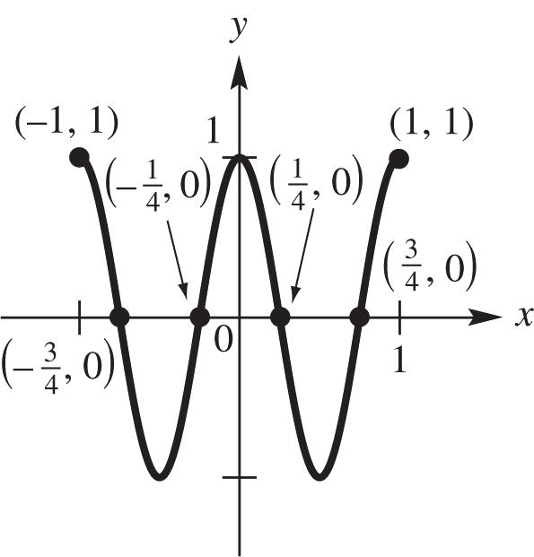
Figure 62a

Figure 62b

Figure 62c
63. (a) The equation ()1yfx is ()yfx shifted 1 unit upward. See Figure 63a.
(b) The equation 30 is ()yfx reflected across the x-axis and shifted 1 unit down. See Figure 63b.
(c) The equation 1 2
is
yfx stretched vertically by a factor of 2 and horizontally by a factor of 2. See Figure 63c.

Figure 63a
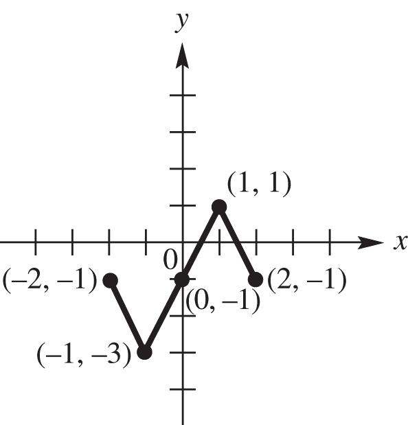
Figure 63b

Figure 63c
64. (a) The equation ()2yfx is ()yfx shifted 2 units downward. See Figure 64a
(b) The equation (1)2yfx is ()yfx shifted 1 unit right and 2 units upward. See Figure 64b.
(c) The equation 2()yfx is ()yfx stretched vertically by a factor of 2. See Figure 64c.
Copyright © 2019 Pearson Education, Inc.
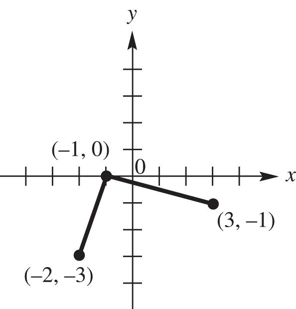
64a
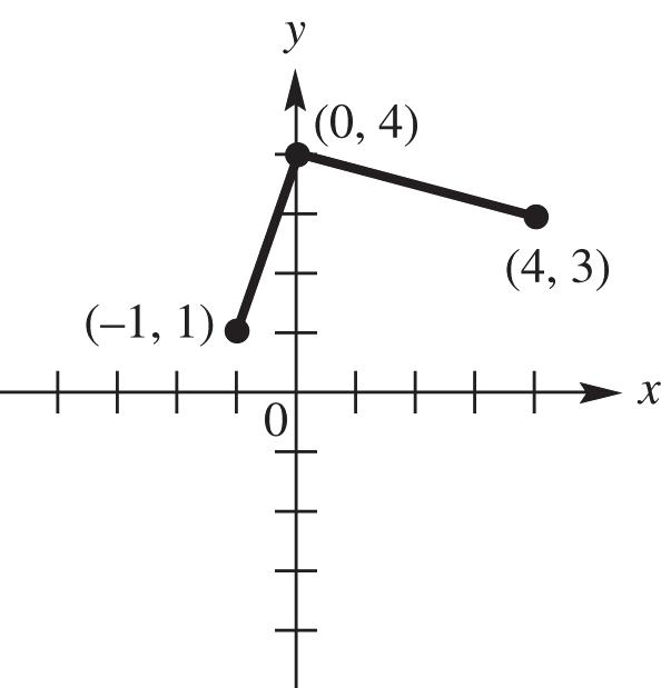
Figure 64b

64c
65. (a) The equation (2)1yfx is x shrunk horizontally by a factor of 2 and shifted 1 unit upward. See Figure 65a.
(b) The equation 1 21 2 yfx
is ()yfx stretched vertically by a factor of 2, stretched horizontally by a factor of 2, and shifted 1 unit upward. See Figure 65b.
(c) The equation 1 (2) 2 yfx is ()yfx shrunk vertically by a factor of 1 2 and shifted 2 units to the right. See Figure 65c.
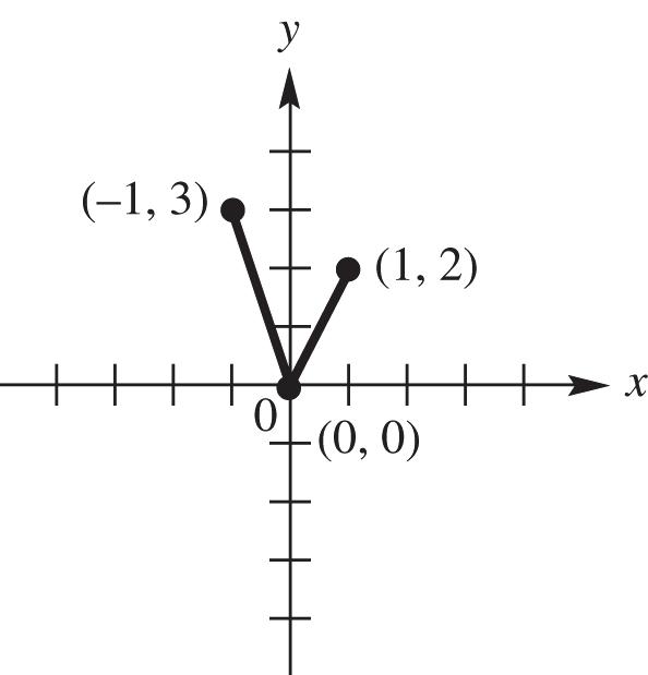
Figure 65a
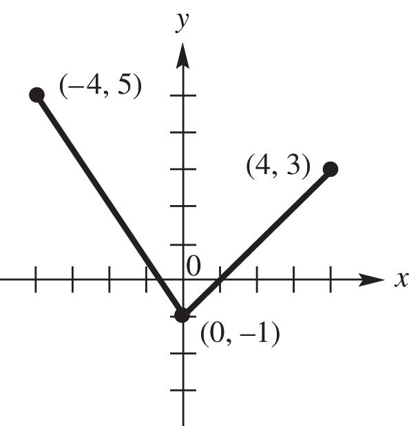
Figure 65b

Figure 65c
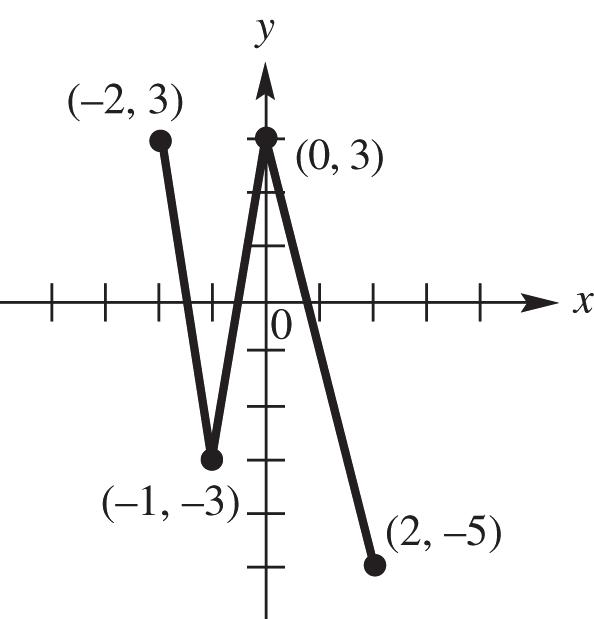
66. (a) The equation (2)yfx is ()yfx shrunk horizontally by a factor of 1 2 See Figure 66a
(b) The equation
stretched horizontally by a factor of 2, and shifted 1 unit downward. See Figure 66b.
(c) The equation 2()1yfx is ()yfx stretched vertically by a factor of 2 and shifted 1 unit downward. See Figure 66c.


67. (a) If (r, 0) is the x-intercept of ()yfx and ()yfx is ()yfx reflected across the x-axis, then (r, 0) is also the x-intercept of ()yfx
(b) If (r, 0) is the x-intercept of ()yfx and ()yfx is ()fx reflected across the y-axis, then ,0 r is the x-intercept of ()yfx
(c) If (r, 0) is the x-intercept of ()yfx and ()yfx is ()yfx reflected across both the x-axis and y-axis, then ,0, r is the x-intercept of ()yfx .
68. (a) If (0,) b is the y-intercept of ()yfx and ()yfx is ()yfx reflected across the x-axis, then 0, b is the y-intercept of ()yfx
(b) If (0,) b is the y-intercept of ()yfx and ()yfx is ()yfx reflected across the y-axis, then (0,) b is also the y-intercept of ()yfx
(c) If (0,) b is the y-intercept of ()yfx and 5()yfx is ()yfx stretched vertically by a factor of 5, then (0,5) b is the y-intercept of 5()yfx
(d) If (0,) b is the y-intercept of ()yfx and 3()yfx is ()yfx reflected across the x-axis and stretched vertically by a factor of 3, then (0,3) b is the y-intercept of 3()yfx
69. Since (2)yfx is ()yfx shifted 2 units to the right, the domain of (2)fx is 12,22 or 1,4 , and the range is the same: 0,3
70. Since 5(1) fx is ()fx shifted 1 unit to the left, the domain of 5(1) fx is 11,21 or 2,1 and, stretched vertically by a factor of 5, the range is 5(0),5(3) or 0,15 .
71. Since ()fx is ()fx reflected across the x-axis, the domain of ()fx is the same: 1,2, and the range is 3,0.
72. Since (3)1fx is ()fx shifted 3 unit to the right, (3)1fx is 13,23 or 2,5, an shifted 1 unit upward, the range is 01,31 or 1,4
Copyright © 2019 Pearson Education, Inc.
73. Since (2)fx is ()fx shrunk horizontally by a factor of 1 2 , the domain of (2)fx is 11 22(1),(2)
or 1 ,1 2
, and the range is the same: 0,3
74. Since 2(1) fx is ()fx shifted 1 unit to the right, the domain of 2(1) fx is 11,21 or 0,3, and stretched vertically by a factor of 3, the range is 2(2),2(3) or 0,6.
75. Since 1 3 4 fx
is ()fx stretched horizontally by a factor of 4 , the domain of 1 3 4 fx
is
4(1),4(2) or 4,8 , and stretched vertically by a factor of 3, the range is 3(0),3(3) or 0,9
76. Since 2(4) fx is ()fx shrunk horizontally by a factor of 1 4 , the domain of 2(4) fx is 11 44(1),(2)
or 11 42,;
and reflected across the x-axis while being stretched vertically by a factor of 2, the range is
2(0),2(3)0,6 or 6,0
77. Since ()fx is ()fx reflected across the y-axis, the domain of ()fx is
(1),(2)1,2 or
2,1; and the range is the same: 0,3
78. Since 2() fx is ()fx reflected across the y-axis, the domain of 2() fx is
(1),(2)1,2 or 2,1, and reflected across the x-axis while being stretched vertically by a factor of 2, the range is
2(0),2(3)0,6 or
6,0
79. Since (3)fx is ()fx reflected across the y-axis and shrunk horizontally by a factor of 1 3 , the domain of (3)fx is 1112 (1),(2), 3333
or 21 , 33
, and the range is the same: 0,3 .
80. Since 1 (3) 3 fx is ()fx shifted 3 units to the right, the domain of 1 (3) 3 fx is 13,23 or 2,5, and shrunk vertically by a factor of 1 , 3 the range is
11
or
0,1.
81. Since yx has an endpoint of (0, 0), and the graph of 10205yx is the graph of yx shifted 20 units right, stretched vertically by a factor of 10, and shifted 5 units upward, the endpoint of 10205yx is 020,1005 or 20,5. Therefore, the domain is [20,) , and the range is [5,).
82. Since yx has an endpoint of (0, 0), and the graph of 21518yx is the graph of yx shifted 15 units left, reflected across the x-axis, stretched vertically by a factor of 2, and shifted 18 units downward, the endpoint of 21518yx is 015,2018 or 15,18. Therefore, the domain is [15,) , and the range, because of the reflection across the x-axis, is ,18.
83. Since yx has an endpoint of (0, 0), and the graph of .5105yx is the graph of yx shifted 10 units left, reflected across the x-axis, shrunk vertically by a factor of .5, and shifted 5 units upward, the endpoint of .5105yx is 010,.505 or 10,5. Therefore, the domain is [10,) , and the range, because of the reflection across the x-axis, is ,5.
84. Using ex. 81, the domain is [,), h and the range is ,. k
85. The graph of ()yfx is ()yfx reflected across the x-axis; therefore, ()yfx is decreasing for the interval ,.ab
86. The graph of ()yfx is ()yfx reflected across the y-axis; therefore, ()yfx is decreasing for the interval , ba .
87. The graph of ()yfx is ()yfx reflected across both the x-axis and y-axis; therefore, ()yfx is increasing for the interval , ba
88. The graph of ()ycfx is ()yfx reflected across the x-axis; therefore, ()ycfx is decreasing for the interval ,.ab
89. (a) the function is increasing for the interval: 1,2 .
(b) the function is decreasing for the interval: ,1.
(c) the function is constant for the interval: 2,.
90. (a) the function is increasing for the interval: ,1.
(b) the function is decreasing for the interval: 1,2.
(c) the function is constant for the interval: 2,.
91. (a) the function is increasing for the interval: 1,.
(b) the function is decreasing for the interval: 2,1.
(c) the function is constant for the interval: ,2.
92. (a) the function is increasing for the interval: ,3.
(b) the function is decreasing for the interval: 3,.
(c) the function is not constant for any interval.
Copyright © 2019 Pearson Education, Inc.
93. From the graph, the point on 2y is approximately 8,10.
94. From the graph, the point on 2y is approximately 27,15.
95. Use two points on the graph to find the slope. Two points are 2,1 and 1,1; therefore, the slope is
The stretch factor is 2 and the graph has been shifted 2 units to the left and 1 unit down; therefore, the equation is 221.yx
96. Use two points on the graph to find the slope. Two points are 1,2 and 5,0; therefore, the slope is 0221 5142
The shrinking factor is 1 , 2 the graph has been reflected across the x-axis, shifted 1 unit to the right, and shifted 2 units upward; therefore, the equation is 1 12. 2 yx
97. Use two points on the graph to find the slope. Two points are 0,2 and 1,1; therefore, the slope is 123 3. 101 mm The stretch factor is 3, the graph has been reflected across the x-axis, and shifted 2 units upward; therefore, the equation is 32.yx
98. Use two points on the graph to find the slope. Two points are 1,2 and 0,1; therefore, the slope is
The stretch factor is 3 and the graph has been shifted 1 unit to the left and 2 units down; therefore, the equation is 312.yx
99. Use two points on the graph to find the slope. Two points are (0,-4) and (3,0); therefore, the slope is 4044 0333
The stretch factor is 4 3 and the graph has been shifted 4 units down.; therefore, the equation is 4 4 3
100. Use two points on the graph to find the slope. Two points are (0,4) and (-3,5); therefore, the slope is 5411
The stretch factor is 1 3 and the graph has been shifted 3 units to the left and 5 units up.; therefore, the equation is 1 35 3 yx .
101. Since ()yfx is symmetric with respect to the y-axis, for every (,) xy on the graph, (,) xy is also on the graph. Reflection across the y-axis reflect onto itself and will not change the graph. It will be the same.
102. The graph is no longer symmetric to the origin since it has been moved away from the origin.
Reviewing Basic Concepts (Sections 2.1—2.3)
1. (a) The function () fxx shifted up one unit yields the function ()1fxx . Therefore, this function has a domain of , and a range of of 1, . The function is increasing from 0, and decreasing from ,0
(b) The function 2 () fxx shifted to the right 2 units yields the function 2 ()2fxx . Therefore, this function has a domain of , and a range of of 0, . The function is increasing from 2, and decreasing from ,2
(c) The function () fxx reflected over the x-axis yields the function () fxx . Therefore, this function has a domain of 0, and a range of of ,0 . The function is never increasing and decreasing from 0,
2. (a) If ()yfx is symmetric with respect to the origin, then another function value is (3)6. f
(b) If ()yfx is symmetric with respect to the y-axis, then another function value is (3)6. f
(c) If ()(),() fxfxyfx is symmetric with respect to both the x-axis and y-axis, then another function value is (3)6. f
(d) If (),yfx ()yfx is symmetric with respect to the y-axis, then another function value is (3)6. f
3. (a) The equation
(b) The equation 2 7 yx is 2 yx shifted 7 units downward: D.
(c) The equation 2 7 yx is 2 yx stretches vertically by a factor of 7: E.
(d) The equation (7)2yx is 2 yx shifted 7 units to the left: A.
(e) The equation
stretches horizontally by a factor of 3: C.
4. (a) The equation 2 2 yx is 2 yx shifted 2 units upward: B.
(b) The equation 2 2 yx is 2 yx shifted 2 units downward: A.
(c) The equation 2 2 yx is
(d) The equation (2)2yx
yx shifted 2 units to the left: G.
shifted 2 units to the right: C.
(e) The equation 2 2 yx is 2 yx stretched vertically by a factor of 2: F.
(f) The equation 2 yx is 2 yx reflected across the x-axis D.
(g) The equation 2 21 yx is 2 yx shifted 2 units to the right and 1 unit upward: H.
(h) The equation 2 21 yx is 2 yx shifted 2 units to the left and 1 unit upward: E.
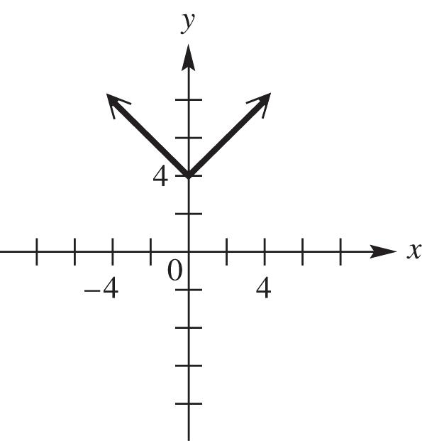
5. (a) The equation 4 yx is yx shifted 4 units upward. See Figure 5a.
(b) The equation 4 yx is yx shifted 4 units to the left. See Figure 5b.
Copyright © 2019 Pearson Education, Inc.
(c) The equation 4 yx is yx shifted 4 units to the right. See Figure 5c.
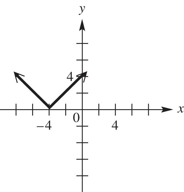
(d) The equation 24 yx is yx shifted 2 units to the left and 4 units down. See Figure 5d.
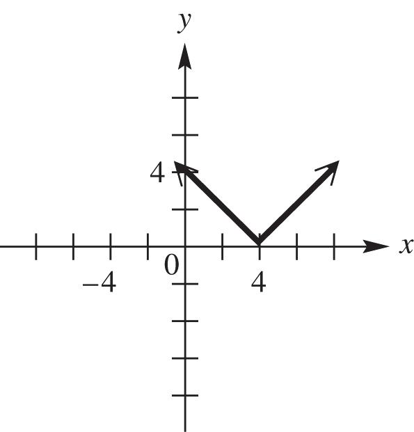
(e) The equation 24 yx is yx reflected across the x-axis, shifted 2 units to the right, and 4 units upward. See Figure 5e.

5d

5e
6. (a) The graph is the function () fxx reflected across the x-axis, shifted 1 unit left and 3 units upward Therefore, the equation is 13. yx
(b) The graph is the function () gxx reflected across the x-axis, shifted 4 units left and 2 units upward. Therefore, the equation is 42. yx
(c) The graph is the function () gxx stretches vertically by a factor of 2, shifted 4 units left and 4 units downward. Therefore, the equation is 244.yx
(d) The graph is the function () fxx shrunk vertically by a factor of 1 , 2 shifted 2 units right and 1 unit downward. Therefore, the equation is 1 21. 2 yx
7. (a) The graph of ()gx is the graph ()fx shifted 2 units upward. Therefore, 2. c
(b) The graph of ()gx is the graph ()fx shifted 4 units to the left. Therefore, 4. c
8. The graph of yFxh is a horizontal translation of the graph of yFx The graph of yFxh is not the same as the graph of , yFxh because the graph of yFxh is a vertical translation of the graph of . yFx
9. (a) If f is even, then ()().fxfx See Figure 9a.
(b) If f is odd, then ()(). fxfx See Figure 9b.
Copyright © 2019 Pearson Education, Inc.

Figure 9a
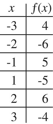
Figure 9b
10. (a) (7)8.25(7)27.585.25 R , In 2017, Google’s ad revenues were $85.25 billion.
(b) Using the point (2010, 27.5) and the slope of 8.255 with the point slope formula we will have 27.58.25(2010)8.25(2010)27.5 yxyx
(c) 8.25(20172010)27.58.25(7)27.585.25 y , In 2017, Google’s ad revenues were $85.25 billion.
(d) 41.5 698.25(2010)27.541.58.25(2010)20102015 8.25 xxxx
11. (a) ()0: {3,4} fx
(b) ()0:fx for the intervals (,3)(4,).
(c) ()0:fx for the interval (3,4).
12. (a) ()0: {2} fx
(b) ()0:fx for the interval 2,.
(c) ()0:fx for the interval ,2.
13. (a) ()0: {4,5} fx
(b) ()0:fx for the intervals ( ] [ ) ,45, -¥-È¥
(c) ()0:fx for the interval [4,5].
14. (a) ()0:fx never; therefore:
(b) ()0:fx for the interval [1,).
(c) ()0:fx never; therefore: .
2.4: Absolute Value Functions
1. We reflect the graph of ()yfx across the x-axis for all points for which 0. y Where 0, y the graph remains unchanged. See Figure 1. The domain and range of ()fx is , and 1, respectively. The domain and range of ()fx is , and 0, respectively.
2. We reflect the graph of ()yfx across the x-axis for all points for which 0. y Where 0, y the graph remains unchanged. See Figure 2. The domain and range of ()fx is , and ,1 respectively. The domain and range of ()fx is , and 0, respectively.
Copyright © 2019 Pearson Education, Inc.
3. We reflect the graph of ()yfx across the x-axis for all points for which 0. y Where 0, y the graph remains unchanged. See Figure 3. The domain and range of ()fx is , and
, respectively. The domain and range of ()fx is
, and 0, respectively.

Figure 1

Figure 2
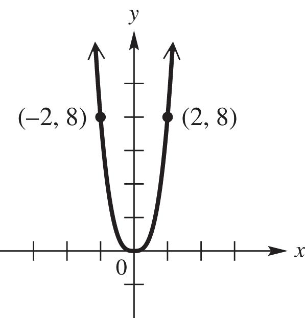
Figure 3
4. We reflect the graph of ()yfx across the x-axis for all points for which 0. y Where 0, y the graph remains unchanged. See Figure 4. The domain and range of ()fx is
, and
, respectively. The domain and range of ()fx is
and
0, respectively.
,
5. Since for all y,y 0, the graph remains unchanged. That is, ()yfx has the same graph as ().yfx The domain and range of ()fx is 0, and 0, respectively. The domain and range of ()fx is
0, and
0, respectively.
6. We reflect the graph of ()yfx across the x-axis for all points for which 0. y Where 0, y the graph remains unchanged. See Figure 6. The domain and range of ()fx is 0, and 0, respectively. The domain and range of ()fx is 0, and 0, respectively.


7. We reflect the graph of ()yfx across the x-axis for all points for which 0. y Where 0, y the graph remains unchanged. See Figure 7. The domain and range of ()fx is ,00, and ,00, respectively. The domain and range of ()fx is ,00, and 0, respectively.
8. We reflect the graph of ()yfx across the x-axis for all points for which 0. y Where 0, y the graph remains unchanged. See Figure 8. The domain and range of ()fx is 0, and 1, respectively.
The domain and range of ()fx is 0, and 0, respectively.
9. We reflect the graph of ()yfx across the x-axis for all points for which 0. y Where 0, y the graph remains unchanged. See Figure 9. The domain and range of ()fx is 2, and 1, respectively. The domain and range of ()fx is 2, and 0, respectively.
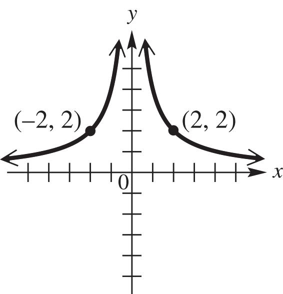
7
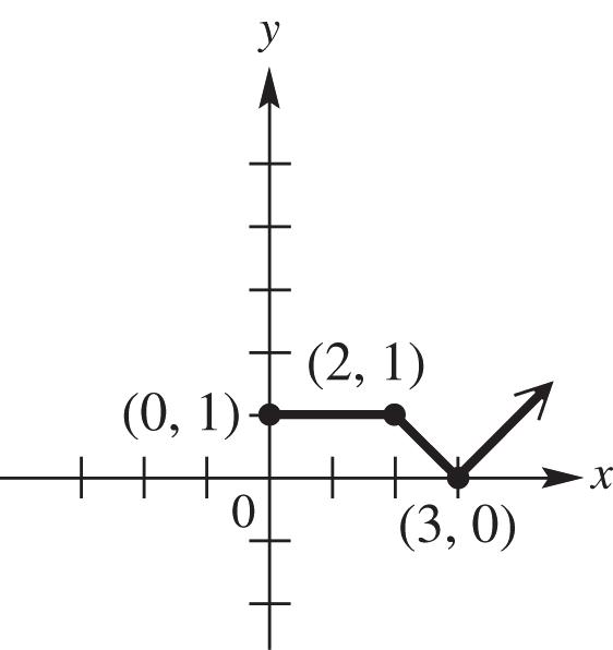
8
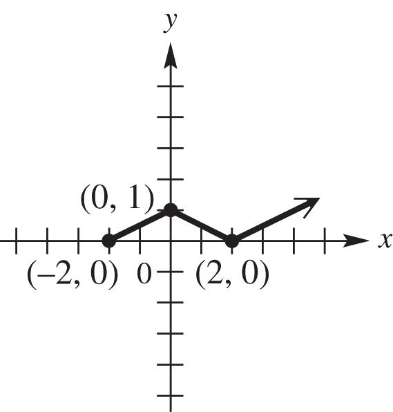
9
10. We reflect the graph of ()yfx across the x-axis for all points for which 0. y Where 0, y the graph remains unchanged.
11. If 5, fa then 55. fa
12. Since 2 fxx is an even function, 2 fxx and 2 fxx are the same graph.
13. If 2 , fxx then 22 yfxyxyx Therefore, the range of yfx is [0,).
14. If the range of ()yfx is [–2, ), the range of yfx is [0,) since all negative values of y are reflected across the x-axis.
15. If the range of ()yfx is ,2, the range of ()yfx is [2,) since all negative values of y are reflected across the x-axis.
16. ()fx is greater than or equal to 0 for any value of x. Since 1 is less than 0, –1 cannot be in the range of f
17 From the graph of 2 (1)2yx the domain of ()fx is (,), and the range is [2,).
From the graph of 2 12 yx the domain of ()fx is (,), and the range is [0,).
18. From the graph of 1 2 2 yx the domain of ()fx is (,), and the range is (,). From the graph of 1 2 2 yx the domain of ()fx is (,), and the range is [0,).
19. From the graph of 2 12yx the domain of ()fx is (,), and the range is (,1]. From the graph of 2 12yx the domain of ()fx is (,), and the range is [1,).
20. From the graph of 22 yx the domain of ()fx is (,), and the range is (,2]. From the graph of 22 yx the domain of ()fx is (,), and the range is [2,).
Copyright © 2019 Pearson Education, Inc.
21. From the graph, the domain of ()fx is 2,3, and the range is 2,3. For the function (),yfx we reflect the graph of ()yfx across the x-axis for all points for which 0 y , and, where 0, y the graph remains unchanged. Therefore, the domain of ()yfx is [–2, 3], and the range is [0, 3].
22. From the graph, the domain of ()fx is [–3, 2], and the range is [–2, 2]. For the function (),yfx we reflect the graph of ()yfx across the x-axis for all points for which 0 y and, where 0, y the graph remains unchanged. Therefore, the domain of ()yfx is [–3, 2], and the range is [0, 2].
23. From the graph, the domain of ()fx is [–2, 3], and the range is [–3, 1]. For the function (),yfx we reflect the graph of ()yfx across the x-axis for all points for which 0 y , and, where 0, y the graph remains unchanged. Therefore, the domain of ()yfx is [–2, 3], and the range is [0, 3].
24. From the graph, the domain of ()yfx is [–3, 3], and the range is [–3, –1]. For the function (),yfx we reflect the graph of ()yfx across the x-axis for all points for which 0 y , and, where 0, y the graph remains unchanged. Therefore, the domain of ()yfx is [–3, 3], and the range is [1, 3].
25. (a) The function ()yfx is the function ()yfx reflected across the y-axis. See Figure 25a.
(b) The function ()yfx is the function ()yfx reflected across both the x-axis and y-axis. See Figure 25b.
(c) For the function ()yfx we reflect the graph of ()yfx (ex. b) across the x-axis for all points for which 0 y , and where 0, y the graph remains unchanged. See Figure 25c.

25a

25b
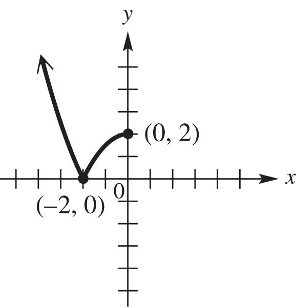
25c
26. (a) The function ()yfx is the function ()yfx reflected across the y-axis. See Figure 26a.
(b) The function ()yfx is the function ()yfx reflected across both the x-axis and y-axis. See Figure 26b
(c) For the function ()yfx we reflect the graph of ()yfx (ex. b) across the x-axis for all points for which 0 y , and, where 0, y the graph remains unchanged. See Figure 26c
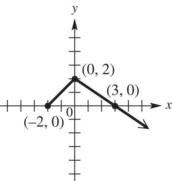
26a
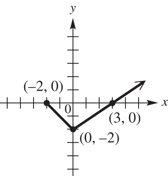
26b

27. The graph of ()yfx can not be below the x-axis; therefore, Figure A shows the graph of (),yfx while Figure B shows the graph of ().yfx
28. The graph of ()yfx can not be below the x-axis; therefore, Figure B shows the graph of (),yfx while Figure A shows the graph of ().yfx
29. See Figure 29a and 29b
30. See Figure 30a and 30b.
31. See Figure 31a and 31b.

29a
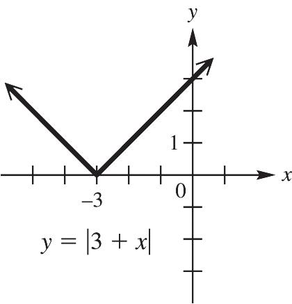
30b
32. See Figure 32a and 32b.
33. See Figure 33a and 33b.
34. See Figure 34a and 34b.
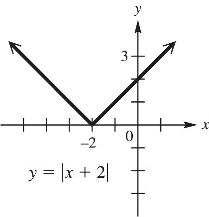
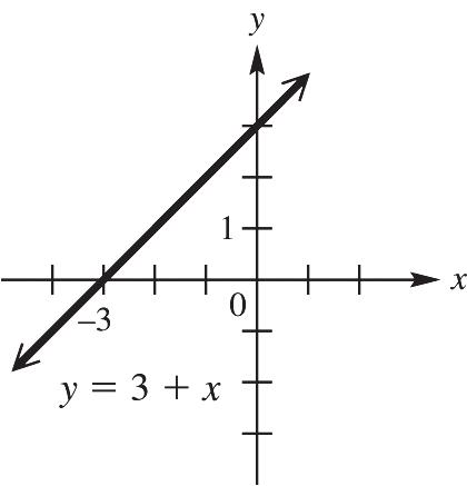

31a
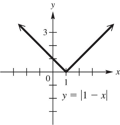
31b
Copyright © 2019 Pearson Education, Inc.
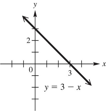
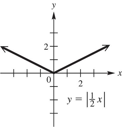
35. See Figure 35a and 35b.
36. See Figure 36a and 36b.
37. See Figure 37a and 37b.

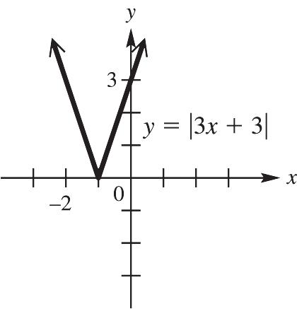
38. See Figure 38a and 38b.
39. See Figure 39a and 39b.
40. See Figure 40a and 40b.
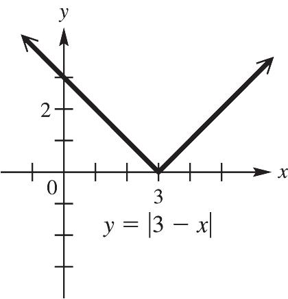
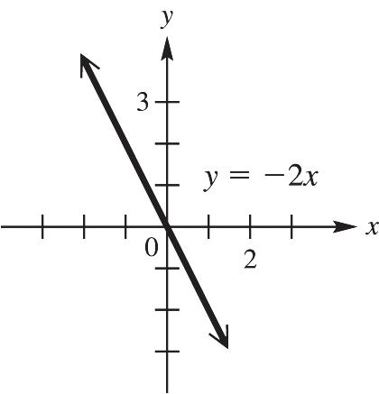

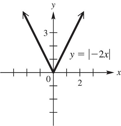

Copyright © 2019 Pearson Education, Inc.
Figure 38a
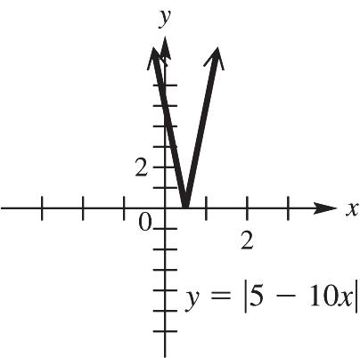
39b
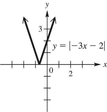
38b
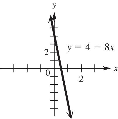
40a

39a
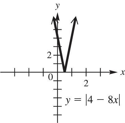
40b
41. (a) From the graph, 12yy at the coordinates 1,5 and 6,5; therefore, the solution set is 1,6.
(b) From the graph, 12yy for the interval 1,6.
(c) From the graph, 12yy for the intervals ,16,.
42. (a) From the graph, 12yy at the coordinates 0,2 and 8,2; therefore, the solution set is 0,8.
(b) From the graph, 12yy for the intervals ,08,.
(c) From the graph, 12yy for the interval 0,8.
43 (a) From the graph, 12yy at the coordinate 4,1; therefore, the solution set is 4.
(b) From the graph, 12yy never occurs; therefore, the solution set is the null set. .
(c) From the graph, 12yy for all values for x except 4; therefore, the solution set is the intervals ,44,.
44. (a) From the graph, 12yy never occurs; therefore, the solution set is
(b) From the graph, 12yy for all values for x; therefore, the solution set is ,.
(c). From the graph, 12yy never occurs; therefore, the solution set is .
45. The V-shaped graph is that of ().56,fxx since this is typical of the graphs of absolute value functions of the form ()|| fxaxb
46. The straight line graph is that of ()314gxx which is a linear function.
47. The graphs intersect at 8,10, so the solution set is 8.
Copyright © 2019 Pearson Education, Inc.
48. From the graph, ()() fxgx for the interval ,8.
49. From the graph, ()() fxgx for the interval 8,.
50. If .563140 xx then .56314. xx Therefore, the solution is the intersection of the graphs, or 8.
51. (a) 4949xx or 495xx or 13. x The solution set is 13,5, which is supported by the graphs of 1 4 yx and 2 9. y
(b) 4949xx or 495xx or 13. x The solution is ,13 5, , which is supported by the graphs of 1 4 yx and 2 9. y
(c) 49949135. xxx The solution is 13,5, which is supported by the graphs of |4| x and 2 9. y
52. (a) 3535xx or 358xx or 2. x The solution set is 2,8, which supported by the graphs of 1 3 yx and 2 5. y
(b) 3535xx or 358xx or 2. x The solution is ,28, which is supported by the graphs of 1 3 yx and 2 5. y
(c) 3553528. xxx The solution is 2,8, which is supported by the graphs of 1 3 yx and 2 5. y
53. (a) 723723 xx or 72324 xx or 2102 xx or 5. x The solution set is 2,5, which is supported by the graphs of 1 72 yx and 2 3. y (b) 723723 xx or 72324 xx or 2102 xx or 5. x The solution set is ,25,, which is supported by the graphs of 1 72 yx and 2 3. y (c) 7233723102452 xxxx
or 25. x The solution is 2,5, which is supported by the graphs of 1 72 yx and 2 3. y
54. (a) 936936 xx
or 936315 xx
or x = -1. The solution set is 5,1, which is supported by the graphs of 1 93 yx and 2 6. y
(b) 936936 xx
or 936315
or 335 xx
or 1. x
The solution is ,51,, which is supported by the graphs of 1 93 yx and 2 6. y
(c) 9366936331515 xxxx
or 51. x The solution is 5,1, which is supported by the graphs of 1 93 yx and 2 6. y
Copyright © 2019 Pearson Education, Inc.
55. (a) 2135212 xx or 21221 xx or 1 23 2 xx
or 3 2 x The solution set is 31 22,,
which is supported by the graphs of 1 213yx and 2 5. y (b) 31 21352212321. 22 xxxx
The solution is 31 22,,
which is supported by the graphs of 1 213yx and 2 5. y
(c) 2135212 xx or 212 x
which is supported by the graphs of 1 213yx and 2
the solution set is ,
which is supported by the graphs of 1 474yx and 2 4.
which is supported by the graphs of 1 57 yx and 2 0. y
(b) 570570 xx or 57075 xx
which is supported by the graphs of 1 57 yx and 2 0. y
(c) 55 5700570575. 77 xxxx The solution set is 5 , 7 which is supported by the graphs of 1 57 yx and 2 0. y
58. (a) Absolute value is always positive; therefore, the solution set is , which is supported by the graphs of 1 8 yx and 2 4. y
(b) Absolute value is always positive, and so cannot be less than 4; therefore, the solution set is , which is supported by the graphs of 1 8 yx and 2 4. y
Copyright © 2019 Pearson Education, Inc.
(c) Absolute value is always positive, and so is always greater than 4; therefore, the solution set is ,, which is supported by the graphs of 1 8 yx and 2 4. y
59. (a) Absolute value is always positive; therefore, the solution set is , which is supported by the graphs of 1 23.6yx and 2 1. y
(b) Absolute value is always positive, and so cannot be less than or equal to 1; therefore, the solution set is , which is supported by the graphs of 1 23.6yx and 2 1. y
(c) Absolute value is always positive, and so is always greater than 1; therefore, the solution is ,, which is supported by the graphs of 1 23.6yx and 2 1. y
60. 24210248248 xxx
or 24824 xx
or 2122 xx
and 6. x Therefore, the solution set is
61. 3434834312434434 xxxx
or 43430
Copyright © 2019 Pearson Education, Inc.
69. 231231 xx or 23124 xx or 2 3(3)45 (3). 9 (3) f g
or 1. x Therefore, the solution is ,12,.
70. 431431 xx or 43133 xx or 351 xx or 5 3 x . Therefore, the solution is
5 ,1, 3
71. 383383 xx or 38335 xx or 5 311 3 xx or 11 3 x Therefore, the solution is 511 ,,. 33
72. Absolute value is always positive, and so is always greater than 1; therefore, the solution is ,.
73. 11 6060 33 xx or 11 606 33 xx or 1 618 3 xx or 18. x Therefore, the solution is every real number except 18: ,1818,.
74. Absolute value is always positive, and cannot be less than 0; therefore, the solution set is
75. Absolute value is always positive, and so cannot be less than or equal to 6; therefore, the solution set is
76. Absolute value is always positive, and so cannot be less than 4; therefore, the solution set is
77. Absolute value is always positive, and so is always greater than 5; therefore, the solution is ,.
78. To solve such an equation, we must solve the compound equation axbcxd or axbcxd . The solution set consists of the union of the two individual solution sets.
79. (a) 3127178
(b) Graph 1 31yx
and 2 27.yx
which is for the interval
(c) Graph 1 31
See Figure 79. From the graph, ()() fxgx
when 12yy
Copyright © 2019 Pearson Education, Inc.
(b) Graph 1 4 yx and 2 712.yx See Figure 80. From the graph, ()() fxgx when 12yy which is for the interval 8 ,1. 3
(c) Graph 1 4 yx and 2 712.yx See Figure 80. From the graph, ()() fxgx when 12yy which is for the interval 8 ,1,. 3
[-20,20] by [-10,50] [-10,10] by [-4,16] Xscl = 2 Yscl = 5 Xscl = 1 Yscl = 1
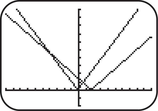
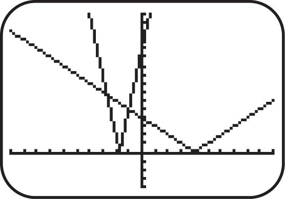
79
Figure 80 81. (a) 2 25332 3 xxxx
the solution
(b) Graph 1225andy3 yxx . See Figure 81. From the graph, ()() fxgx when 12yy , which it is for the
(c) Graph 1225andy3 yxx See Figure 81. From the graph, ()() fxgx when 12yy , which it is for the interval 2 ,8 3
. Therefore, the solution set is 35 , 28
(b) Graph 1 51yx and 2 34.yx See Figure 82. From the graph, ()() fxgx when 12yy , which it is for the interval 35 ,,. 28
(c) Graph 1 51yx and 2 34yx . See Figure 82. From the graph, ()() fxgx when 12yy , which it is for the interval 35 28,.
Copyright © 2019 Pearson Education, Inc.

Figure 81
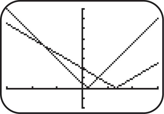
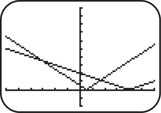
(b) Graph 1 3 yx and 2 1 8 3 yx . See Figure 84. From the
(c) Graph 1 3 yx and 2 1 8 3 yx . See Figure 84. From the graph, ()() fxgx when 12yy , which it is for the interval 3315
(b). Graph 1 41yx or 2 y46.
See Figure 85. From the graph ()() fxgx when 12yy , which it is for the interval 7 , 8
(c) Graph 1 41yx or 2 y46. x See Figure 85. From the graph, ()() fxgx when 12yy , which is for the interval 7 , 8
. [-10,10] by [-10,10] [-10,10] by [-10,10] [-10,10] by [-10,10] Xscl = 1 Yscl = 1 Xscl = 1 Yscl = 1 Xscl= 1 Yscl = 1
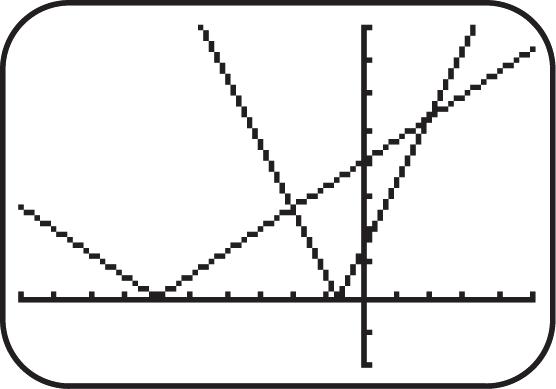
Figure 84

Figure 85
86. (a) 696393 xx

Figure 86
Therefore, the solution set is 1 2
(b) Graph 12 69 and63yxyx . See Figure 86. From the graph, ()() fxgx when 12yy , which it is for the interval 1 ,. 2
(c) Graph 12 69 and63yxyx . See Figure 86. From the graph, ()() fxgx when 12yy , which it is for the interval 1 ,. 2
87. (a) 0.2510.7530.5048 xxxx or 0.251(0.753) xx 0.2510.753 xx
2. x Therefore, the solution set is 2,8.
(b) Graph 12 .251 and.753.yxyx See Figure 87. From the graph, ()() fxgx when 12yy , which it is for the interval (2,8).
(c) Graph 12 .251 and.753.yxyx See Figure 87. From the graph, ()() fxgx when 12yy , which it is for the interval ,28,.
88. (a) .402.60520735 xxxx or .402(.605) xx .402.6053 xxx . Therefore, the solution set is 3,35.
(b) Graph 12 .402 andy.605yxx . See Figure 88. From the graph, ()() fxgx when 12yy , which it is for the interval (3,35).
(c ) Graph 12 .402 andy.605yxx . See Figure 88. From the graph, ()() fxgx when 12yy , which it is for the interval ,335,
Copyright © 2019 Pearson Education, Inc.
[-20,20] by [-4,16] [-30,50] by [-5,30] [-10,10] by [-10,10] [-10,10] by [-10,10]
Xscl = 2 Yscl = 1 Xscl = 5 Yscl = 5 Xscl= 1 Yscl = 1 Xscl = 1 Yscl = 1
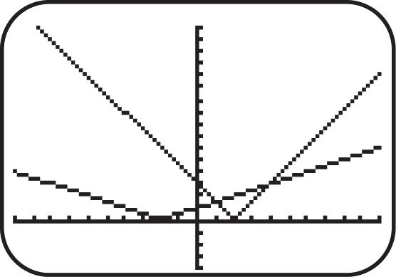
Figure 87

Figure 88

Figure 89
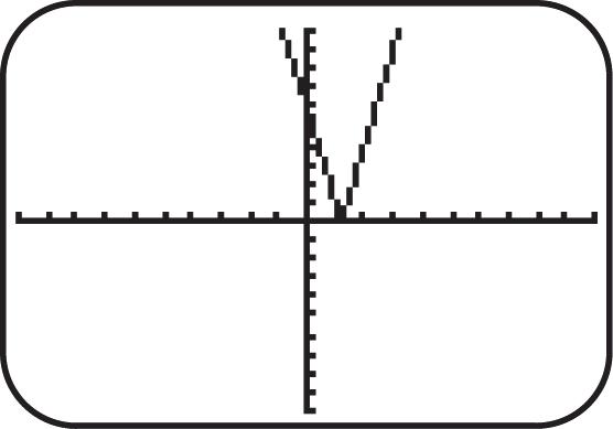
Figure 90
89. (a) 310(310)310310 xxxx there are an infinite number of solutions.
Therefore, the solution set is , .
(b) Graph 12 310 andy310yxx . See Figure 89. From the graph, ()() fxgx when 12yy , for which there is no solution.
(c ) Graph 12 310 andy310yxx . See Figure 89. From the graph, ()() fxgx when 12yy , for which there is no solution.
90. (a) 56(56)5656 xxxx there are an infinite number of solutions.
Therefore, the solution set is , .
(b) Graph 12 56 andy56yxx . See Figure 90. From the graph, ()() fxgx when 12yy , for which there is no solution.
(c ) Graph 12 56 andy56yxx . See Figure 90. From the graph, ()() fxgx when 12yy , for which there is no solution.
91. Graph 1 16yxx and 2 11. y See Figure 91 From the graph, the lines intersect at (3,11) and (2,9). Therefore, the solution set is 3,8.
92. Graph 1 221yxx and 2 9. y See Figure 92. From the graph, the lines intersect at (4,9) and (2,9). Therefore, the solution set is 4,2.
93. Graph 1 4 yxx and 2 8. y See Figure 93. From the graph, the lines intersect at (2,8) and (6,8). Therefore, the solution set is 2,6.
94. Graph 1 .52.254yxx and 2 9. y See Figure 94. From the graph, the lines intersect at (20,9) and (4,9). Therefore, the solution set is 20,4.
Copyright © 2019 Pearson Education, Inc.
[-10,10] by [-4,16] [-10,10] by [-4,16] [-10,10] by [-4,16] [-30,10] by [-4,16] Xscl = 1 Yscl = 1 Xscl = 1 Yscl = 1 Xscl= 1 Yscl = 1 Xscl = 5 Yscl= 1
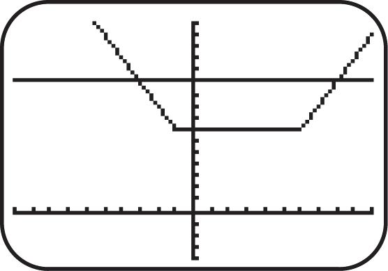
Figure 91
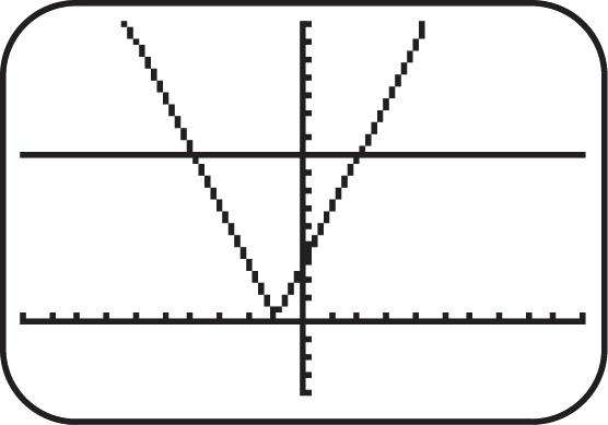
Figure 92

Figure 93
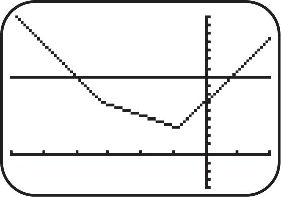
Figure 94
95. (a) 50222250222872. TTT
(b) The average monthly temperatures in Boston vary between a low of 28 F and a high of 72 F. The monthly averages are always within 22 of 50 F.
96. (a) 10363610362646. TTT .
(b) The average monthly temperatures in Chesterfield vary between a low of 26 F and a high of 46 F.
The monthly averages are always within 36 of 10 F.
97. (a) 61.512.512.561.512.54974. TTT
(b) The average monthly temperatures in Buenos Aires vary between a low of 49 F (possibly in July) and a high of 74 F (possibly in January). The monthly averages are always within 12.5 of 61.5 F.
98. (a) 43.58.58.543.58.53552. TTT
(b) The average monthly temperatures in Punta Arenas vary between a low of 35 F and a high of 52 F.
The monthly averages are always within 8.5 of 43.5 F.
99. (a) The max circumference is 10.1 and the minimum circumference is 9.9. This can be represented as 100.1 C (b)
102. (a)
103. (a) 4840.04 x
Copyright © 2019 Pearson Education, Inc.
Chapter 2: Analysis of Graphs of Functions
(b) 4840.044120.040.044120.0411.96412.04 xxxx 2.993.01 x
104. (a)
512100.1 x (b) 512100.15220.10.15220.121.9522.1 xxxx 4.384.42 x
105. (a)
40.50.001 x (b)
40.50.0014.50.0010.0014.50.0014.4994.501 xxxx
106. (a) 71.20.002 x (b)
71.20.0025.80.0020.0025.80.0025.8025.798 xxxx 5.7985.802 x
107. 8.01.51.58.01.56.59.5; xxx therefore, the range is the interval 6.5,9.5.
108. If 680780 730 2 is the midpoint, then 680780680730730780730 FF
507305073050 FF
109. (a) 11612599dd
(b) 1712012017or12017137orP=103 PPPP
.
110. If 98148 123 2 is the midpoint, then 9814898123123123148123 xxx
2512325|123|25 xx (or 12325 x ); and if 1626 2 21 is the midpoint, then 16261621212621 xx 5215 x 215 x (or 215 x ).
11. If 2761 xx then 27(61)0. xx Graph 1 27(61),yxx See Figure 111. The x -intercept is 2; therefore, the solution set is 2.
112. If 3121 xx then 312(1)0. xx Graph 1 312(1),yxx See Figure 112. The equation is 0, or the graph intersects or is above the x-axis, for the interval: 2.75,6.5.
113. If 4.56xx then 4.560.xx Graph 1 4.56,yxx See Figure 113. The equation is 0, or the graph is above the x-axis, for the interval: (,).
114. If 2834 xx then 28340. xx Graph 1 2834,yxx See Figure 114. The equation is 0, or the graph is above the x-axis, for the interval: (,).
Copyright © 2019 Pearson Education, Inc.
[-10,10] by [-10,10] [-10,10] by [-10,10] [-10,10] by [-10,10] [-10,10] by [-4,16]
Xscl = 1 Yscl = 1 Xscl = 1 Yscl = 1 Xscl= 1 Yscl = 1 Xscl = 1 Yscl= 1
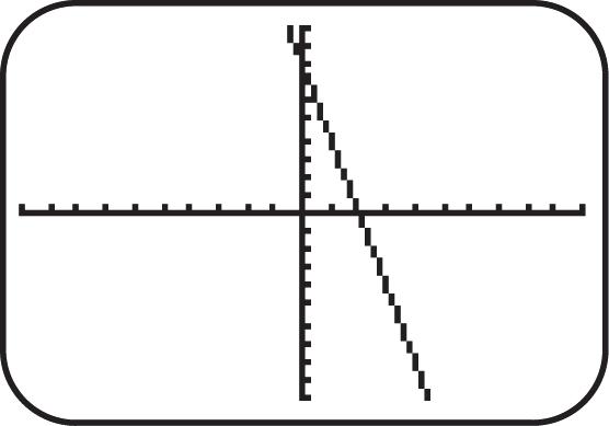
Figure 111
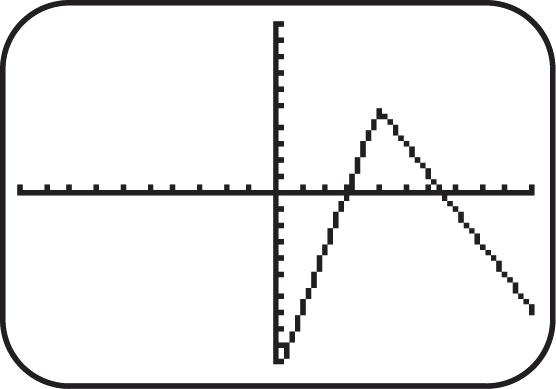
Figure 112

113
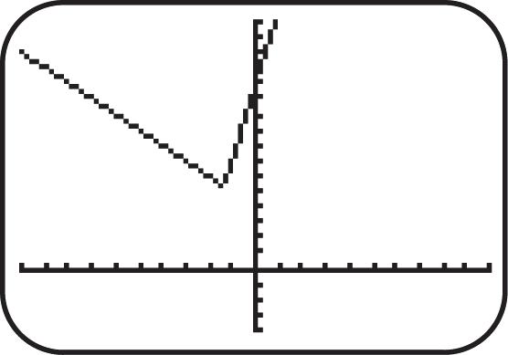
114
115. If 34314 xx then 343140. xx Graph 1 34314,yxx See Figure 115. The equation is 0, or the graph is below the x-axis, never or for the solution set: .
116. If 13610xx then 136100.xx Graph
1 13610yxx See Figure 100. The equation is 0, or the graph intersects or is below the x-axis, never or for the solution set:
[-10,10] by [-10,10] [-10,10] by [-10,10] Xscl = 1 Yscl = 1 Xscl = 1 Yscl = 1

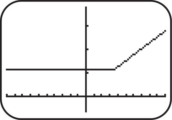
2.5: Piecewise-Defined Functions
1. (a) From the graph, the speed limit is 40 mph.
(b) From the graph, the speed limit is 30 mph for 6 miles.
(c) From the graph, (5)40mph; f (13)30mph; f and (19)55mph. f
(d) From the graph, the graph is discontinuous at 4,6,8,12,and16. x The speed limit changes at each discontinuity.
2. (a) From the graph, the Initial amount was: $1,000; and the final amount was: $600.
(b) From the graph, (10)$900;(50)$600. ff The function f is not continuous.
(c) From the graph, the discontinuity shows 3 drops or withdrawals.
(d) From the graph, the largest drop or largest withdrawal of $300 occurred after 15 minutes.
(e) From the graph, the one increase or deposit was $200.
3. (a) From the graph, the Initial amount was: 50,000 gal.; and the final amount was: 30,000 gal.
(b) From the graph, during the first and fourth days.
(c) From the graph, (2)45,000gal;(4)40,000gal ff .
Copyright © 2019 Pearson Education, Inc.
(d) From the graph, between days 1 and 3 the water dropped: 50,00040,00010,000 5,000 22 gal./day.
4. (a) From the graph, when x = 1 the tank had 20 gallons of gas.
(b) Since x = 0 represents 3:15 pm and 3 hours later the tank was filled to 20 gallons, the time was 6:15 pm
(c) When the graph is horizontal, the engine is not running; when the graph is decreasing, the engine is burning gasoline; and when the graph is increasing, gasoline is being put into the tank.
(d) When the graph is decreasing, gasoline was burned the fastest between 1 and 2.9 hours
5. (a)
7. (a) (5)2(5)3 f
(0)(0)0 f
8. (a) (5)2(5)10 f
(c) (0)3(0)11 f
(b) (1)3(1)14 f
9. Yes, continuous. See Figure 9.
10. Yes, continuous. See Figure 10.
11. Not continuous. See Figure 11
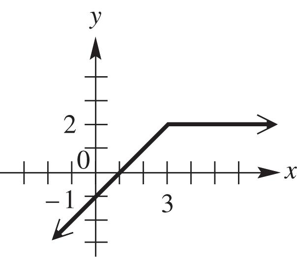
Figure 9
12. Not continuous. See Figure 12.
13. Not continuous. See Figure 13.
14. Not continuous. See Figure 14.
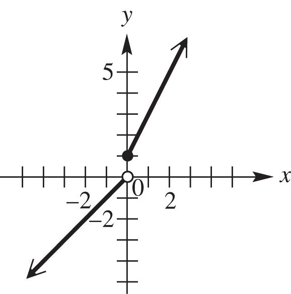
Figure 12
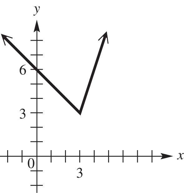
Figure 10

Figure 11

Figure 13
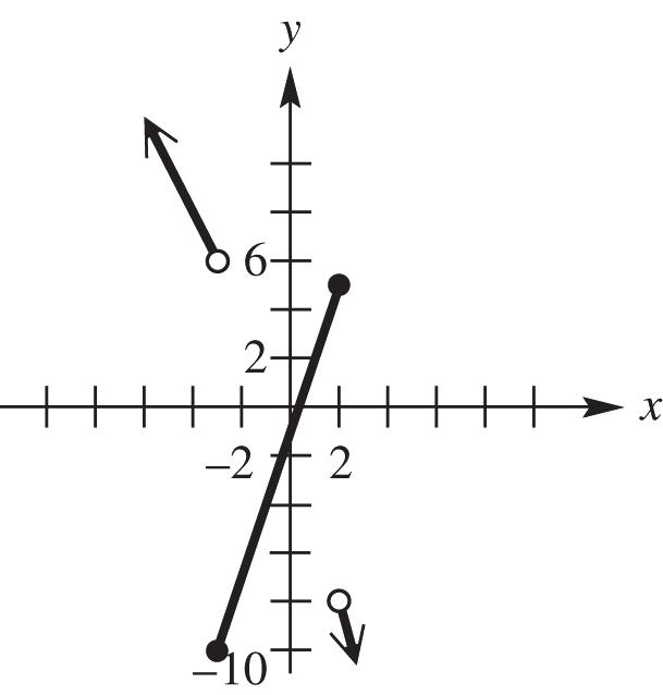
Figure 14
Copyright © 2019 Pearson Education, Inc.
15. Not continuous. See Figure 15.
16. Not continuous. See Figure 16.
17. Yes, continuous. See Figure 17.
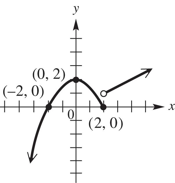
15
18. Not continuous. See Figure 18.
19. Yes, continuous. See Figure 19.
20. Yes, continuous. See Figure 20.

18
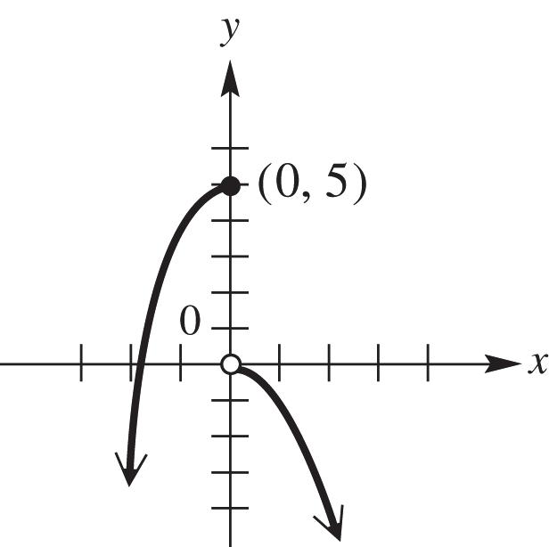
16

17
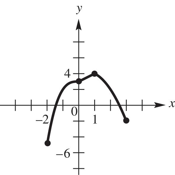
19

20
21. Look for a 2 yx graph if 0; x and a linear graph if 0 x . Therefore: B.
22. Look for a yx graph if 1; x and a reflected 2 yx graph if 1 x . Therefore: A.
23. Look for a horizontal graph above the x-axis if 0; x and a horizontal graph below the x-axis if 0 x .Therefore: D.
24. Look for a yx graph if 0; x and a reflected 2 yx graph if 0 x .Therefore: C.
25. Graph 1 (1)(3)(2)(3),yxxx See Figure 25.
26. Graph 1 (6)(3)(36)(3),yxxxx See Figure 26.
27. Graph 1 (4)(2)(12)(2),yxxxx See Figure 27.
28. Graph 1 (21)(0)()(0),yxxxx See Figure 28.
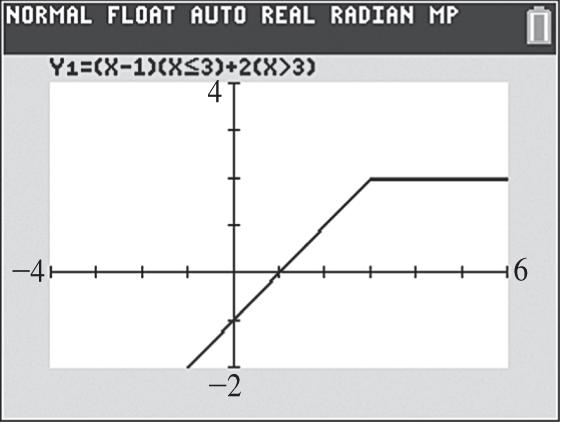
Figure 25
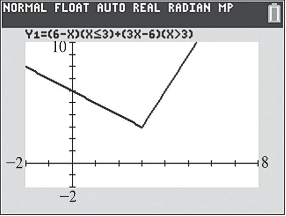
Figure 26
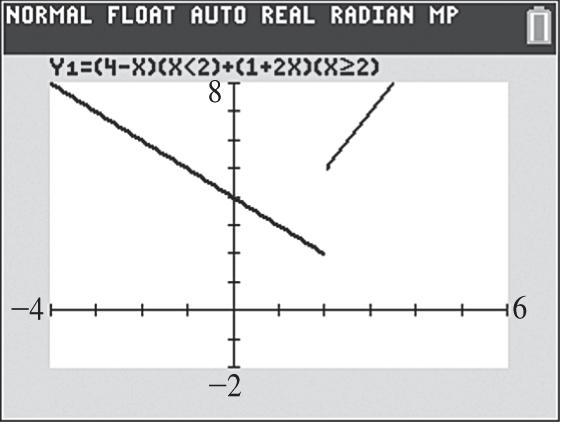
Figure 27
29. Graph 1 (2)(4)()(4and5)(3)(5), yxxxxxxx
See Figure 29.
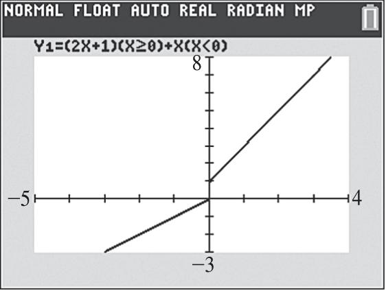
Figure 28
30. Graph 1 (2)(3)(31)(3and2)(4)(2), yxxxxxxx See Figure 30.
31. Graph 1 11 222(2)(2),yxxxx
See Figure 31.
32. Graph 32 1 (5)(0)()(0),yxxxx See Figure 32.


Figure 29
33. From the graph, the function is
34. From the graph, the function
35. From the graph, the
36. From the graph, the function
37. From the graph, the function is
38. From the graph, the function is
39. There is an overlap of intervals since the number 4 satisfies both conditions. To be a function, every x-value is used only once.
40. The value (4) f cannot be found since using the first formula, (4)11, f and using the second formula, (4)16. f To have two different values violates the definition of function.
41. The graph of yx = is shifted 1.5 units downward.
42. The graph of yx = is reflected across the y-axis.
43. The graph of yx = is reflected across the x-axis.
44. The graph of yx = is shifted 2 units to the left.
45. Graph 1.5, yx=- See Figure 45.
46. Graph , yx =- See Figure 46.
47. Graph , yx =- See Figure 47.
48. Graph 2, yx=+ See Figure 48.

Figure 45
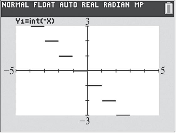
Figure 46
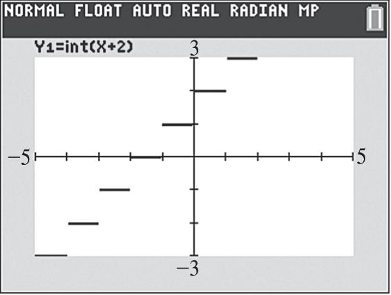
Figure 47
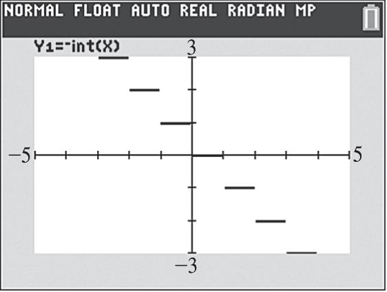
Figure 48
49. (a) In 2012 there were 200 million users (2012, 200) and in 2015 there were 700 million users (2015, 700). The slope is given as 700200500 201520123 . The equation is given as
500 2002012 3 Wx
500 2012200 3 Wx between 2012 and 2015 inclusively. In 2018 there were 1000 million users (2018, 1000). The slope is given as 1000700300 100 201820153
The equation is 7001002015Wx 100(2015)700Wx between 2015 and 2018.
(b) See Figure 49. The function is continuous on this time period.
(c) From 2012 to 2015, the number of active WhatsApp users increased , on average, by about 166.7 million users per year. From 2015 to 2018, this increase slowed to 100 million per year, on average.
50. (a) In January 2014 there were 46 million users (0, 46) and in July 2015 there were 94 million users (17, 94). The slope is given as 9446488 180183 . The equation is given as 8 46 3 Sx between 0 and 18 months inclusively.
Copyright © 2019 Pearson Education, Inc.
In January 2017 there were 160 million users (36, 160). The slope is given as 160946611 3618183 . The equation is given as 1111 160(36)28 33 SxSx between 18 and 36 months.
(b) See Figure 50. The function is continuous on the time interval.
(c) From January 2014 to July 2015, the number of daily active Snapchat users increased, on average, by about 2.7 million per month. From July 2015 to January 2017, this increased to 3.7 million per month, on average.

Figure 49

Figure 50
51. When 03 x the slope is 5, which means the inlet pipe is open and the outlet pipe is closed; when 35 x the slope is 2, which means both pipes are open; when 58 x the slope is 0, which means both pipes are closed; when 810 x the slope is 3 , which means the inlet pipe is closed and the outlet pipe is open.
52. (a) Since for each year given the shoe size is 1 size smaller than his age, the formula is 1 yx
(b) From the table and question, graph the function. See figure 50.
53. (a) (1.5)0.70,(3)0.91, ff It costs $0.70 to mail 1.5 oz and $0.91 to mail 3 oz.
(b) Domain: 0,5; Range: 0.49,0.70,0.91,1.12,1.33 . See figure 53.
54. (a) (1967)0.0475(1967)93.30.1325 f , In 1967, the average Super Bowl ad cost $0.1325 million.
(b) (1998)0.475(1998)93.31.605 f , In 1998, the average Super Bowl ad cost $1.605 million.
(c) (2013)0.179(2013)356.0375.01 f , In 2013, the average Super Bowl ad cost $5.01 million
(d) The function ()fx is continuous on its domain since there are no breaks in the graph of ()fx .
(e) See Figure 54.
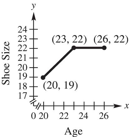
Figure 52
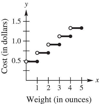
Figure 53
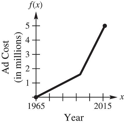
Figure 54
Copyright © 2019 Pearson Education, Inc.
55. (a) From the table, graph the piecewise function. See Figure 55.
(b) The likelihood of being a victim peaks from age 16 up to age 20, then decreases.
56. (a) From the table, graph the piecewise function. See Figure 56.
(b) Housing starts increased, decreased, and increased, with the maximum occurring during the 1960’s.
57. (a) From the graph, the highest speed is 60 mph and the lowest speed is 20 mph.
(b) There are approximately 4 miles of highway with a speed of 55 mph.
(c) Fromt the graph, (4)40;(12)20;(18)7. fff
56. From the table, graph the piecewise function. See Figure 56.

Figure 55

Figure 56
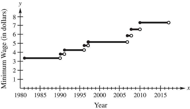
Figure 58
59. (a) A 3.5 minute call would round up to 4 minutes. A 4 minute call would cost: .503(.25)$1.25.
(b) We use a piecewise defined function where the cost increases after each whole number as follows: .50if 01 .75if 12 () 1.00if 23 1.25if 34 1.50if 45 x x fxx x x
. Another possibility is
.50if 01 () .50.251if 15 x fx xx
60. (a) Since cost is rounded down to the nearest 2 foot interval, we can use the greatest integer function. The function is ().80 2 fxx =
(b) Graph ().80 2 fxx =
(c)
from 618. x ££
from 618. x ££ See Figure 60.
8.5 (8.5).80.804.25.80(4)(8.5)$3.20 2 ff====
15.2 (15.2).80.807.6.80(7)(15.2)$5.60 2 ff
Copyright © 2019 Pearson Education, Inc.
[6,18] by [0,8]
Xscl = 1 Yscl = 1

Figure 60
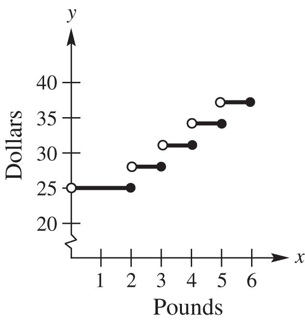
61. For x in the interval 0,2,25. y For x in the interval 2,3,25328. y For x in the interval 3,4,28331 y and so on. The graph is a step function. In this case, the first step has a different width. See Figure 61.
62. Sketch a piecewise function that measures miles over minutes. The first piece increases at a rate of 40 mph or 402 603 miles per minute, for 30 minutes (the time it takes to travel 20 miles at that rate). The second piece stays at a constant distance of 20 miles for the 2 hour period at the park. The third piece decreases (returns home) at a rate of 20 mph or 201 603 miles per minute, for 60 minutes (the time it takes to travel 20 miles at that rate). See Figure 62.
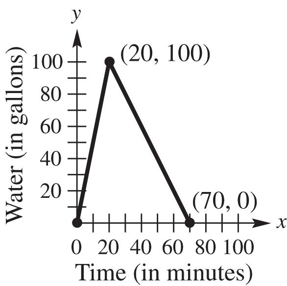
63. Sketch a piecewise function that fills a tank at a rate of 5 gallons a minute for the first 20 minutes (the time it takes to fill the 100 gallon tank) and then drains the tank at a rate of 2 gallons per minute for 50 minutes (the time it takes to drain the 100 gallon tank). See Figure 63.

64. (a) Use the points (1990, 1.3) and (2007, 2.7) to find the slope. 2.71.31.4 0.082 2007199017
11()1.30.082(1990)0.082161.88 yymxxyxyx
Use the points (2007, 2.7) and (2016, 1.5) to find the slope. 1.52.71.2 0.13 201620079 m
1.50.13(2016)0.13263.58 yxyx
(b) Use the two functions above to create 0.082161.8819902007 () 0.13263.5820072016
Copyright © 2019 Pearson Education, Inc.
2.6: Operations and Composition
1. 22(25)25. xxxxE
2. 22(25)25. xxxxB
3. 232 (25)25. xxxxF
4. 2 . 25 x D x
5. 22 (25)42025 xxxA
6. 22 (2()5)25. xxC
7. 2 (3)((3))(2(3)1)(5)53(5)40fgfgff
8. 2 (2)((2))((2)3(2))(2)2(2)15gfgfgg
9. 222 ()(())(21)(21)3(21)44163422 fgxfgxfxxxxxxxx
10. 222 ()(())(3)2(3)1261 gfxgfxgxxxxxx
11. 2 3(3)(3)((3)3(3))(2(3)1)23fgfg
12. 2 (5)(5)(5)53(5)(2(5)1)1fgfg
13.
14.
15.
16.
2 (4)(4)(4)43(4)2(4)1196fgfg
2 13(1) (1)2 (1) (1)2(1)13
2 43(4) (4)28 (4)4 (4)2(4)17
22. Because the two compositions are opposites of each other.
23. (a)
()()(41)(63)102 fgxxxx , ()()(41)(63)24 fgxxxx 22 ()()(41)(63)2412632463 fgxxxxxxxx
(b) All values can replace x in all three equations; therefore, the domain is (,) in all cases.
(c) 41 (); 63 fx x gx
all values can replace x, except 1 ; 2 therefore, the domain is 11 ,,. 22
(d)
()()()4(63)1241212411; fgxfgxxxx all values can be input for x; therefore, the domain is (,)
(e)
24. (a)
()()()6(41)32463243; gfxgfxxxx all values can replace x; therefore, the domain is (,)
()()(92)(52)711 fgxxxx , ()()(92)(52)37 fgxxxx
22 ()()(92)(52)4518104104918 fgxxxxxxxx
(b) All values can replace x in all three equations; therefore, the domain is (,) in all cases.
(c) 92 (); 52 fx x gx
all values can replace x, except 2 5 ; therefore, the domain is 22 ,,. 55
(d) ()()()92(52)9104105; fgxfgxxxx all values can replace x; therefore, the domain is (,)
(e) ()()()5(92)2451021043; gfxgfxxxx all values can replace x; therefore, the domain is (,)
25. (a) ()()32 fgxxx , ()()32 fgxxx , ()()3(2) fgxxx
(b) All values can replace x in all three equations; therefore, the domain is (,) in all cases.
(c) 3 (); 2 fx x gx
all values can replace x, except 0; therefore, the domain is (,0)(0,)
(d) ()()()(2)323; fgxfgxxx all values can replace x; therefore, the domain is (,). (e) ()()()2323; gfxgfxxx all values can replace x; therefore, the domain is (,)
26. (a) ()()24(1)241 fgxxxxx , ()()24(1)241 fgxxxxx ()()24(1)(1)24 fgxxxxx
(b) All values can replace x in all three equations; therefore, the domain is (,) in all cases.
(c) 24 () 1 fx x gx
all values can replace x, except 1; therefore, the domain is (,1)(1,).
(d) ()()()2(1)422; fgxfgxxx all values can replace x, so the domain is (,).
(e) ()()()241; gfxgfxx all values can replace x, so the domain is (,).
Copyright © 2019 Pearson Education, Inc.
27. (a) 3333 ()()4(5)45 fgxxxxx , 3333 ()()4(5)45 fgxxxxx 3 3 ()()4(5) fgxxx
(b) All values can replace x in all three equations; therefore, the domain is (,) in all cases.
(c) 3 3 4 () (5) fx x gx
all values can replace x, except 3 5 , so the domain is 33 (,5)(5,).
(d) 3 33 3 ()()()(5)49; fgxfgxxx all values can replace x, so the domain is (,).
(e) 3 3 ()()()45459; gfxgfxxxx all values can replace x, so the domain is (,). 28. (a)
3333 ()()63(21)6321 fgxxxxx
3333 ()()63(21)6321 fgxxxxx
3 3 ()()63(21) fgxxx
(b) All values can replace x in all three equations; therefore, the domain is (,) in all cases.
(c) 3 3 63 (); (21) fx x gx
all values can replace x, except 3 1 2 , so the domain is 33 11 ,, 22
(d)
(e)
3 33 3 ()()()63(21)63; fgxfgxxx all values can replace x, so the domain is (,).
3 3 ()()()26312(63)1613; gfxgfxxxx all values can replace x; therefore, the domain is (,).
29. (a) 22 ()()3(1)31 fgxxxxx , 22 ()()3(1)31 fgxxxxx 2 ()()3(1) fgxxx
(b) All values can replace x in all three equations; therefore, the domain is (,) in all cases.
(c) 2 3 (); (1) fx x gx
all values can replace x, except 1; therefore, the domain is ,11,
(d) 222 ()()()(1)321324; fgxfgxxxxxx all values can replace x; therefore, the domain is (,).
(e) 22 ()()()3131; gfxgfxxx all values can replace x; therefore, the domain is, (,).
Copyright © 2019 Pearson Education, Inc.
30. (a) ()()24()2422 fgxxxxx , ()()24()2422 fgxxxxx ()()24()2422 fgxxxxx
(b) All values can replace x in all three equations; therefore, the domain is (,) in all cases.
(c) 2 24 ();fx x gx
all values can replace x, except 0; therefore, the domain is ,00,.
(d) 22 ()()()24()24; fgxfgxxx all values can replace x; therefore, the domain is (,).
(e) 22 ()()()2424; gfxgfxxx all values can replace x; therefore, the domain is (,).
31. (a) From the graph, 4(2)2.
(b) From the graph, 1(3)4.
(c) From the graph, (0)(4)0.
(d) From the graph, 11 . 33
32. (a) From the graph, 022.
(b) From the graph, 213.
(c) From the graph, (2)(1)2.
(d) From the graph, 4 2. 2
33. (a) From the graph, 033.
(b) From the graph, 145.
(c) From the graph, (2)(1)2.
(d) From the graph, 3 0 undefined.
34. (a) From the graph, 312.
(b) From the graph, 202.
(c) From the graph, (3)(1)3.
(d) From the graph, 3 3. 1
35. (a) From the table, 7(2)5.
(b) From the table, 1055.
(c) From the table, (0)(6)0.
(d) From the table, 5 0 undefined.
Copyright © 2019 Pearson Education, Inc.
36. (a) From the table, 549.
(b) From the table, 000.
(c) From the table, (4)(2)8.
(d) From the table, 8 8. 1
37. See Table 37.
38. See Table 38.


39. (a) ()(4)(4), fgfg so from the graph find (4)0. g Now find (0)4; f therefore, ()(4)4. fg
(b)
()(3)(3), gfgf so from the graph find (3)2. f Now find 22; g therefore, ()(3)2. gf
(c) ()(2)(2), ffff so from the graph find (2)0. f Now find (0)4; f therefore, ()(2)4. ff
40. (a) ()(2)(2), fgfg so from the graph find (2)2. g Now find (2)4; f therefore, ()(2)4. fg
(b) ()(0)(0), gggg so from the graph find (0)2. g Now find (2)2; g therefore, ()(0)2. gg
(c) ()(4)(4), gfgf so from the graph find (4)2. f Now find (2)2; g therefore, ()(4)2. gf
41. (a) ()(1)(1), fgfg so from the graph find (1)2. g Now find (2)3; f therefore, ()(1)3. fg
(b)
()(2)(2), gfgf so from the graph find (2)3. f Now find (3)2; g therefore, ()(2)2. gf
(c) ()(2)(2), gggg so from the graph find (2)1. g Now find (1)0; g therefore, ()(1)0. gg
42. (a) ()(2)(2), fgfg so from the graph find (2)4. g Now find (4)2; f therefore, ()(2)2. fg
(b)
(c)
43. (a)
(b)
()(1)(1), gfgf so from the graph find (1)1. f Now find (1)1; g therefore, ()(1)1. gf
()(0)(0), ffff so from the graph find (0)0. f Now find (0)0; f therefore, ()(0)0. ff
()(1)(1), gfgf so from the table find (1)4. f Now find (4)5; g therefore, ()(1)5. gf
()(4)(4), fgfg so from the table find (4)5. g (5) f is undefined; therefore, ()(4) fg is undefined.
Copyright © 2019 Pearson Education, Inc.
2: Analysis of Graphs of Functions
(c) ()(3)(3), ffff so from the table find (3)1. f Now find (1)4; f therefore, ()(3)4. ff
44. (a) ()(1)(1), gfgf so from the table find (1)2. f Now find (2)4; g therefore, ()(1)4 gf . (b) ()(4)(4), fgfg so from the table we find 4 g is undefined; therefore, ()(4) fg is undefined.
(c) ()(3)(3), ffff so from the table find (3)6. f Now find (6)7; f therefore, ()(3)7. ff
45. From the table, (3)4 g and (4)2. f
46. From the table, (6)7 f and (7)0. g
47. Since 312 YYY and 1, X we solve 12 (1). YY First solve 2 2 (1)1, Y now solve 1 2153; Y therefore, 3 3. Y
48. Since 312 YYY and 2, X we solve 12 (2). YY First solve 2 2 (2)4, Y now solve 1 2(4)53; Y therefore, 3 3. Y
49. Since 312 YYY and 7, X we solve 12 (7). YY First solve 2 2 749, Y now solve 1 2(49)593; Y therefore, 3 93. Y
50. Since 312 YYY and 8, X we solve 12 (8). YY First solve 2 2 864, Y now solve 1 2(64)5123; Y therefore, 3 123. Y
51. (a)
23 ()()()(31); fgxfgxxx all values can be input for x; therefore, the domain is (,). (b) 32363 ()()()()3()131; gfxgfxxxxx all values can be input for x; therefore, the domain is (,).
(c) 339 ()()()(); ffxffxxx all values can be input for x; therefore, the domain is (,).
52. (a) 22 11 ()()()22; fgxfgx xx
all values can be input for x, except 0; therefore, the domain is (,0)(0,).
(b) 2 1 ()()(); (2) gfxgfx x all values can be input for x, except 2; therefore, the domain is (,2)(2,).
(c) ()()()2(2); ffxffxxx all values can be input for x; therefore, the domain is (,).
53. (a) 2 ()()()11; fgxfgxxx all values can be input for x; therefore, the domain is (,).
(b) 22 ()()()1()1; gfxgfxxx only values where 2 1 x can be input for x; therefore, the domain is 1,1.
(c) 224 ()()()(); ffxffxxx all values can be input for x; therefore, the domain is (,).
Copyright © 2019 Pearson Education, Inc.
54. (a) 4242 ()()()(34)232; fgxfgxxxxxxx all values can be input for x; therefore, the domain is (,).
(b) 42 ()()()(2)(2)3(2)4; gfxgfxxxx all values can be input for x; therefore, the domain is (,).
(c) ()()()(2)24; ffxffxxx all values can be input for x; therefore, the domain is (,).
55. (a) 11 ()()[()]; (5)151 fgxfgx
all values can be input for x, except 1 ; 5 therefore, the domain is 11 ,,. 55
(b) 15 ()()[()]5; 11 gfxgfx xx
all values can be input for x, except, −1; therefore, the domain is (.1)(1,). (c) 1111 ()()[()]; 112 1 2 1 111 1 ffxffxx
all values can be input for x, except those that make 1 0 2 x x or undefined. That would be −1 and −2; therefore, the domain is (,2)(2,1)(1,).
56. (a) 22 ()()[()](4)444; fgxfgxxx only values where 2 4 x can be input for x; therefore, the domain is [−2, 2].
(b) 2 ()()[()]4(4); gfxgfxx only values where 2 (4)4 x can be input for x; therefore, the domain is [−6, −2].
(c) ()()[()](4)48; ffxffxxx all values can be input for x; therefore, the domain is (,).
57. (a) 3232 ()()[()]2(45)18101; fgxfgxxxxx all values can be input for x; therefore, the domain is (,).
(b) 32 ()()[()]4(21)5(21) gfxgfxxx 322 4(81261)5(441) xxxxx 32232 3248244(20205)322841; xxxxxxxx all values can be input for x; therefore, the domain is (,).
(c) ()()[()]2(21)143; ffxffxxx all values can be input for x; therefore, the domain is (,).
58. (a) (23)32 ()()[()]; 23 fxx gxfgxx all values can be input for x; therefore, the domain is (,).
Copyright © 2019 Pearson Education, Inc.
(b) 3 ()()[()]23(3)3; 2 x gfxgfxxx
all values can be input for x; therefore, the domain is (,).
all values can be input for x; therefore, the domain is (,).
59. (a) ()(())(5)5,fgxfgxf
all values can be input for x, thefore the domain is ,
.
(b) ()(())(5)5,gfxgfxg all values can be input for x, therefore the domain is
(c) ()(())(5)5,ffxffxf all values can be input for x, therefore the domain is ,
60. (a) 1 ()()[()] 1 fgxfgx x all values can but 1 can be input for x; therefore, the domain is
,11,.
(b) 11 ()()[()]1 gfxgfxx xx
all values but 0 can be input for x; therefore, the domain is ,00,.
(c) 1 ()()[()] 1 ffxffxx x all values can be input for x; therefore, the domain is (,).
61. (a) 1 ()()[()] 2 fgxfgx x all values can but 4 can be input for x; therefore, the domain is
,44,.
(b) 112 ()()[()] 22 2 gfxgfxx xx x
all values bigger than 2 can be input for x; therefore, the domain is
all values but 5 2 can be input for x; therefore, the domain is 55 ,,. 22
62. (a) 11 ()()[()] 36146 fgxfgx xx
all values can but 2 3 can be input for x; therefore, the domain is 22 ,,. 33
Copyright © 2019 Pearson Education, Inc.
(b) ()()[()]3631611 gfxgfx xx
all values but –1 can be input for x; therefore, the domain is ,11,.
()()[()]
all values but 2 can be input for x; therefore, the domain is
63. Let () fxc
then
Therefore, there is only one value in the range of ()ffx
64. Let () fxk and g()xmxb
Therefore, there is only one value k in the range of ()fgx
65. 1 ()()[()]4(2)222 4
66.
69. Graph 3 3 12 6, 6, yxyx and 3 yx in the same viewing window. See Figures 69. The graph of 2 y can be obtained by reflecting the graph of 1y across the line 3 .yx
70. Graph 12 1 53, 3, 5 yxyx and 3 yx in the same viewing window. See Figures 70. The graph of 2 y can be obtained by reflecting the graph of 1y across the line 3 .yx [-10,10] by [-10,10] [-10,10] by [-10,10] Xscl = 1 Yscl = 1 Xscl = 1 Yscl = 1
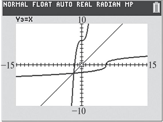
Figure 69

Figure 70
71. (a) 2222 ()4()()424; fxxfxhxhxxhh
Copyright © 2019 Pearson Education, Inc.
(b)
Chapter 2: Analysis of Graphs of Functions
2222 ()()448 fxfhxhxh
72. (a) 222222 ()5()5()()5(2)()5105; fxxxfxhxhxhxxhhxhxxhhxh (b)
73. (a)
2222 ()()5555 fxfhxxhhxxhh
222222 ()3()3()()332233 fxxxfxhxhxhxhxxhhxxhxhh ; (b)
74. (a)
2222 ()()3333 fxfhxxhhxxhh
()()()23333223223 fxxfxhxhxxhhxhxhxhxh (b) 33 ()() fxfhxh
75. Using fxhfx h gives:
76. Using fxhfx h gives:
77. Using
gives:
443434
Using
= 2 1 4 1 2 4. 2 xhhh xh h
79. Using ()() fxhfx h gives: 3332233223 22 ()3333 33. xhxxxhxhhxxhxhh xxhh hhh
80.
81. Using ()() fxhfx h gives:
Copyright © 2019 Pearson Education, Inc.
82. Using ()() fxhfx h gives:
83. Using ()() fxhfx h gives:
84. Using ()() fxhfx h gives:
85. Using ()() fxhfx h gives:
2(22)2 11 222222 1 2()2 2() xxhh xhxxxhxxh hhhxxh
86. Using ()() fxhfx h gives:
222222 22 ()22 11 () xxhxxxhhxhh xhxxxhxxhxxh
87. One possible solution is 2 () fxx and ()62.gxx Then 2 ()()[()](62). fgxfgxx
88. One possible solution is 2 () fxx and 2 ()1112. gxxx Then 22 ()()[()](1112). fgxfgxxx
89. One possible solution is () fxx and 2 ()1.gxx Then 2 ()()[()]1. fgxfgxx
90. One possible solution is 3 () fxx and ()23.gxx Then 3 ()()[()](23). fgxfgxx
91. One possible solution is ()12fxx and ()6. gxx Then ()()[()]612. fgxfgxx
92. One possible solution is 3 ()4fxx and ()23.gxx Then 3 ()()[()]234. fgxfgxx
93. (a) There are 5280 feet in a mile. ()5280 Fxx
(b) There are 12 inches in a foot. ()12 Ixx
(c) ()()(())I(5280)12(5280)63,360 IFxIFxxxx
(d) The number of inches in a mile.
94. (a) There are 2000 pounds in a ton. ()2000 Txx
(b) There are 16 ounces in a pound. ()16 Oxx
(c) ()(())(2000)16(2000)32,000 OTxOTxOxxx
(d) The number of ounces in a ton.
95. (a) With a cost of $10 to produce each item and a fixed cost of $500, the cost function is ()10500.Cxx
(b) With a selling price of $35 for each item, the revenue function is ()35. Rxx
(c) The profit function is ()()()()35(10500)()25500. PxRxCxPxxxPxx
(d) A profit is shown when ()02550002550020. Pxxxx Therefore, 21 items must be produced and sold to realize a profit.
(e) Graph 1 25500.yx The smallest whole number for which ()0Px is 21. Use a window of [0,30] by [1000,500], for example.
96. (a) With a cost of $11 to produce each item and a fixed cost of $180, the cost function is ()11180.Cxx
(b) With a selling price of $20 for each item, the revenue function is ()20. Rxx
(c) The profit function is ()()()()20(11180)()9180. PxRxCxPxxxPxx
(d) A profit is shown when ()091800918020. Pxxxx Therefore, 21 items must be produced and sold to realize a profit.
(e) Graph 1 9180.yx The smallest whole number for which ()0Px is 21. Use a window of [5,30] by [200,200], for example.
97. (a) With a cost of $100 to produce each item and a fixed cost of $2700, the cost function is ()1002700.Cxx
(b) With a selling price of $280 for each item, the revenue function is ()280. Rxx
(c) The profit function is ()()()()280(1002700)()1802700. PxRxCxPxxxPxx
(d) A profit is shown when ()018027000180270015. Pxxxx
Therefore, 16 items must be produced and sold to realize a profit.
(e) Graph 1 1802700,yx the smallest whole number for which ()0Px is 16. Use a window of [0,30] by [3000,500], for example.
98. (a) With a cost of $200 to produce each item and a fixed cost of $1000, the cost function is ()2001000.Cxx
(b) With a selling price of $240 for each item, the revenue function is ()240. Rxx
(c) The profit function is ()()()()240(2001000)()401000. PxRxCxPxxxPxx
(d) A profit is shown when ()0401000040100025. Pxxxx Therefore, 26 items must be produced and sold to realize a profit.
(e) Graph 1 401000,yx the smallest whole number for which ()0Px is 26. Use a window of [5,40] by [1200,600], for example.
99. (a) If 3 4 (), 3 Vrr then a 3 inch increase would be 3 4 ()(3), 3 Vrr and the volume gained would be 4433 ()(3). 33 Vrrr
(b) Graph 33 1 44 (3) 33 yxx in the window [0,10] by [0,1500]. See Figure 99. Although this appears to be a portion of a parabola, it is actually a cubic function.
(c) From the graph in exercise 91b, an input value of 4 x results in a gain of 1168.67. y
Copyright © 2019 Pearson Education, Inc.
(d) 33 444413722561116 (4)(43)(4)(343)(64)3721168.67. 3333333 V
100. If 2 ()4,Srr then doubling the radius would give us a surface area gained function of 22222 ()4(2)416412. Srrrrrr
101. (a) If x width, then 2 x length. Since the perimeter formula is 22 PWL our perimeter function is ()2()2(2)24()6. PxxxxxPxx This is a linear function.
(b) Graph ()6 Pxx in the window [0,10] by [1,100]. See Figure 101b. From the graph when 4,24.xy The 4 represents the width of a rectangle and 24 represents the perimeter.
(c) If 4 x is the width of a rectangle then 28 x is the length. See Figure 101c. Using the standard perimeter formula yields 2(4)2(8)24. P This compares favorably with the graph result in part b.
(d) (Answers may vary.) If the perimeter y of a rectangle satisfying the given conditions is 36, then the width x is 6. See Figure 101d.

99
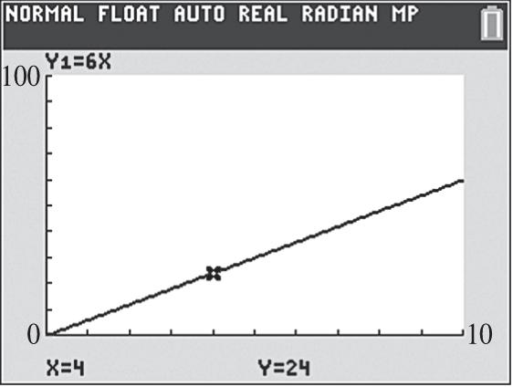
101b
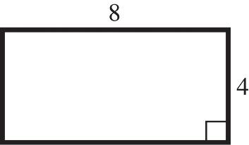
102. (a) If 4 xs then . 4 x s
(b) If 2 ys and , 4 x s then
()(). 416 xx yxyx
(c) Sine x is the perimeter and 2 (6)369 6,(6)2.25. 16164 xy
(d) Show that the point (6,2.25) is on the graph
A square with perimeter 6 will have area 2.25 square u nits.
103. (a) 33222 (2)(2)(4)(2)3 44 AxxxAxx
(b) 2 33 ()(16)(256)()643 44 AxAx
square units.
(c) On the graph of 2 3 , 4 yx locate the point where 16 x to find 110.85, y an approximation for 643.
Copyright © 2019 Pearson Education, Inc.
104. (a) If 2 () Arr and ()2 rtt then 22 ()()[()][2](2)4. ArtArtAttt
(b) ()() Art is a composite function that expresses the area of the circular region covered by the pollutants as a function of time t (in hours).
(c) Since 0 t is 8 A.M., noon would be 22 4.()(4)4(4)64mi.tAr
(d) Graph 2 1 4 yx and show that for 4,201xy (an approximation for 64).
105. (a) (2100)42,A ; The average age of a person in 2100 is projected to be 42 years. (2100)430 T , In 2100, the living world’s population will have a combined life experience of 430 billion years.
(b) (2100)430 10.2 (2100)42 T A , The world population will be about 10.2 billion in 2100.
(c) P(x) gives the world’s population during year x.
106. (a) The domain is the years. See table below. Therefore, D= { 2013, 2014, 2015, 2016 }.
(b) The function h computes the number of acres of soybeans harvested in the U.S. in millions of acres.
107. (a) ()(2010)13.074.387.3 fg
(b) The function ()() fgx computes the total SO2 and Carbon Monoxide during year x
(c) Add functions f and g
108. (a) The function h is the addition of functions f and g
(b) The function h is the addition of functions f and g. Therefore, ()()(). hxfxgx
109. (a) The function h is the subtraction of function f from g. Therefore, ()()(). hxgxfx (b) (2000)(2000)(2000)403010 hgf
, (2014)(2014)(2014)1008020 hgf
(c) Using the points (2014, 100) and (2000, 40), the slope is 100406030 20142000147 m The equation is 30 1002014 7 yx Using the points (2014, 80) and (2000, 30), the slope is
Copyright © 2019 Pearson Education, Inc.
. The difference between the two equations is given as
110. (a) Graph
in the window [1982, 1994] by [0, 1] See Figure 11-a.
Approximately 59% of the people who contracted AIDS during this time period died.
(b) Divide number of deaths by number of cases for each year. The results compare favorably with the graph. See Figure 110b. Xscl = 1 Yscl = 1
110a
Reviewing Basic Concepts (Sections 2.4—2.6)
1.
Therefore, the solution set is 12,4.
(b) 111 242424 222 xxxx
Therefore, the solution interval is (,12)(4,). (c) 111 2442462124. 222 xxxx
Therefore, the solution interval is [-12,4].
2. For the graph of |()|,yfx we reflect the graph of ()yfx across the x-axis for all points for which 0. y Where 0, y the graph remains unchanged. See Figure 2.

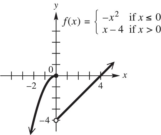
3. 3 2413241353or24(13)24315 5 xxxxxxxxxxx
The solution set is 3 ,5 5
4. (a) (3)2(3)33 f (b) 2 (0)(0)44 f (c) 2 (2)(2)48 f
5. (a) See Figure 5a.
(b) Graph 2 1 ()*(0)(4)*(0)yxxxx in the window [-10,10] by [-10,10]. See Figure 5b. [-10,10] by [-10,10] Xscl = 1 Yscl = 1
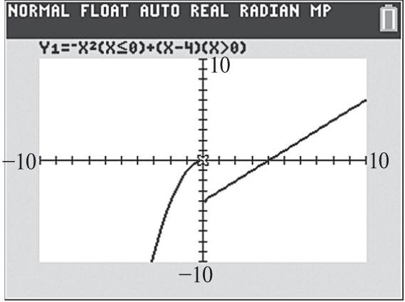
5b
6. (a) 22 ()()(34)()34. fgxxxxx Therefore, 2 ()(1)(1)3(1)46. fg
(b) 22 ()()(34)()34. fgxxxxx Therefore, 2 ()(3)(3)3(3)422. fg
(c) 232 ()()(34)()34. fgxxxxx Therefore, 32 ()(1)3(2)4(2)24168. fg
(d) 2 34 ().fx x gx
Therefore, 2 3(3)45 (3). 9 (3)
(e) 22 ()()[()]3()4()()34 fgxfgxxfgxx
(f) 22 ()()[()](34)()()92416 gfxgfxxgfxxx
7. (a) ()()[()]4 fgxfgxx
(b) (g)()[f()]4fxgxx
8. One of many possible solutions for ()()() fgxhx is 4 () fxx and ()2.gxx Then 4 ()()[()](2). fgxfgxx
9. 22222 2()3()5(235)2(2)335235 xhxhxxxxhhxhxx hh 2222 242335235423 423. xxhhxhxxxhhh xh hh
10. (a) At 4% simple interest the equation for interest earned is 1 .04.yx
(b) If he invested x dollars in the first account, then he invested x+500 in the second account. The equation for the amount of interest earned on this account is 22.025(500).02512.5. yxyx
(c) It represents the total interest earned in both accounts for 1 year.
Copyright © 2019 Pearson Education, Inc.
Section 2.R 139
(d) Graph 1212.04(.02512.5).04.02512.5 yyxxyyxx in the window [0,1000] by [0,100]. See Figure 10. An input value of 250, x results in $28.75 earned interest.
(e) At 12 250,.04(250).025(250)12.5106.2512.5$28.75.xyy [0,1000] by [-20,100] Xscl = 100 Yscl = 10
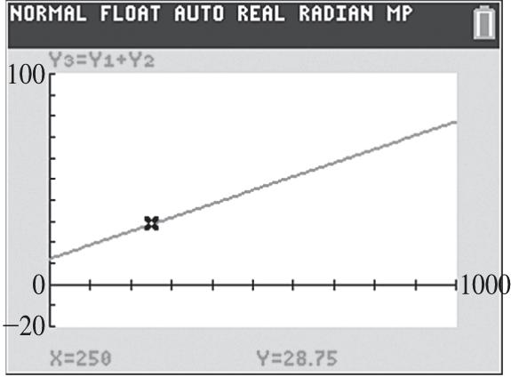
Figure 10
11. If the radius is r, then the height is 2r and the equation is 222222 (2)455.SrrrrrrrrSr
Chapter 2 Review Exercises
The graphs for exercises 1–10 can be found in the “Function Capsule” boxes located in section 2.1 in the text.
1. True Both 2 () fxx and ()||fxx have the interval: [0,) as the range.
2. True Both 2 () fxx and ()||fxx increase on the interval: [0,) .
3. False The function () fxx has the domain: [0,) and 3 () fxx the domain: (,)
4. False The function 3 () fxx increases on its entire domain.
5. True The function () fxx has a domain and range of: (,)
6. False The function () fxx is not defined on (,0) , so certainly cannot be continuous.
7. True All of the functions show increases on the interval: [0,)
8. True Both () fxx and 3 () fxx have graphs that are symmetric with respect to the origin.
9. True Both 2 () fxx and ()||fxx have graphs that are symmetric with respect to the y-axis.
10. True No graphs are symmetric with respect to the x-axis.
11. Only values where 0 x can be input for x, therefore the domain of () fxx is: [0,)
12. Only positive solution are possible in absolute value functions, therefore the range of () fxx is: [0,)
13. All solution are possible in cube root functions, therefore the range of 3 () fxx is: (,)
14. All values can be input for x, therefore the domain of 2 () fxx is: (,)
15. The function 3 () fxx increases for all inputs for x, therefore the interval is: (,)
16. The function ()||fxx increases for all inputs where 0 x , therefore the interval is: [0,)
17. The equation is the equation yx . Only values where 0 x can be input for x, therefore the domain of yx is: [0,)
Copyright © 2019 Pearson Education, Inc.
18. The equation 2 yx is the equation yx Square root functions have both positive and negative solutions and all solution are possible, therefore the range of yx is: (,)
19. The graph of ()(3)1fxx is the graph yx shifted 3 units to the left and 1 unit downward.
See Figure 19.
20. The graph of 1 ()1 2 fxx is the graph reflected yx across the x-axis, vertically shrunk by a factor of 1 2 , and shifted 1 unit upward. See Figure 20.
21. The graph of 2 ()(1)2fxx is the graph 2 yx shifted 1 unit to the left and 2 units downward.
See Figure 21.
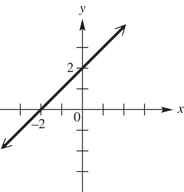
Figure 19

Figure 20
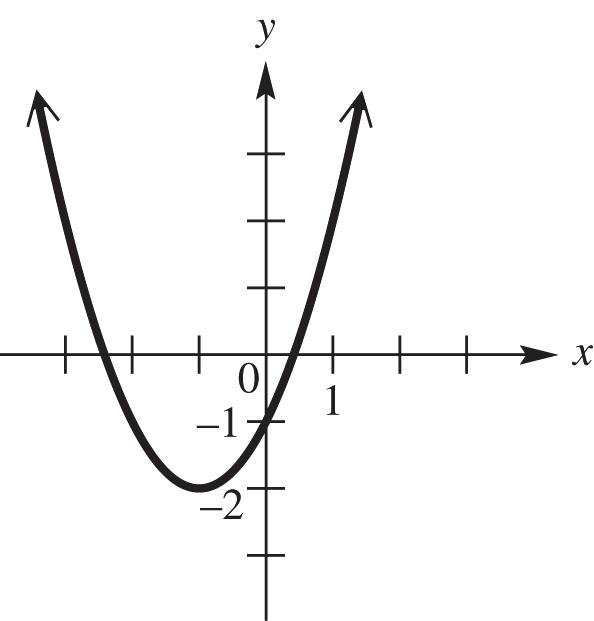
Figure 21
22. The graph of 2 ()23fxx is the graph 2 yx reflected across the x-axis, vertically stretched by a factor of , and shifted 3 units upward. See Figure 22.
23. The graph of 3 2 fxx is the graph 3 yx reflected across the x-axis and shifted 2 units upward.
See Figure 23.
24. The graph of 3 3 fxx is the graph 3 yx shifted 3 units to the right. See Figure 24.
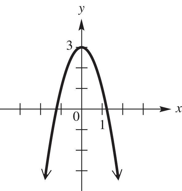
Figure 22
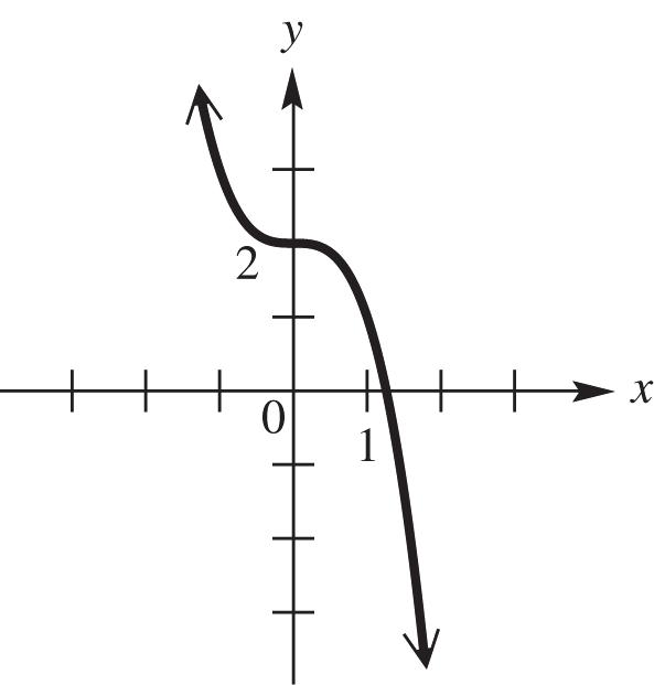
Figure 23
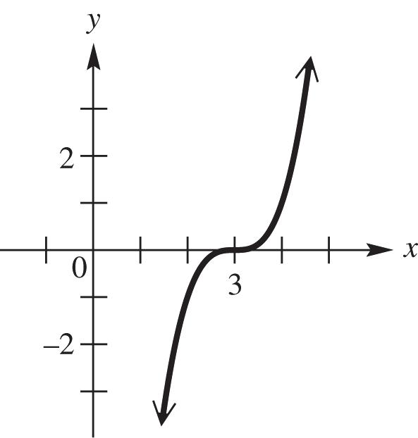
Figure 24
25. The graph of 1 2 fxx is the graph yx horizontally stretched by a factor of 2. See Figure 25.
26. The graph of 21 fxx is the graph yx shifted 2 units to the right and 1 unit upward.
See Figure 26.
Copyright © 2019 Pearson Education, Inc.
27. The graph of 3 2 fxx is the graph 3 yx vertically stretched by a factor of . See Figure 27.
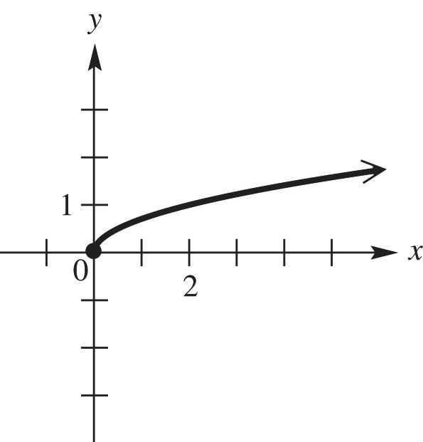
Figure 25
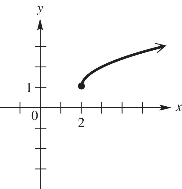
Figure 26
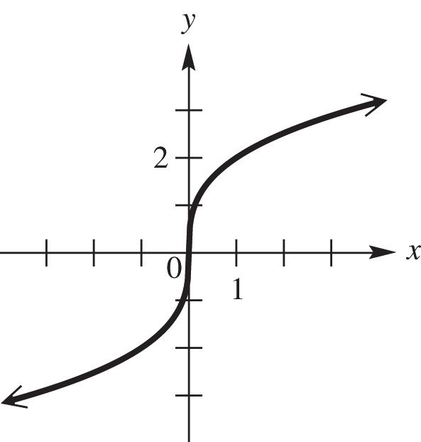
Figure 27
28. The graph of 3 2 fxx is the graph 3 yx shifted 2 units downward. See Figure 28.
29. The graph of |2|1fxx is the graph ||yx shifted 2 units right and 1 unit upward. See Figure 29.
30. The graph of |23|fxx is the graph ||yx horizontally shrunk by a factor of 1 2 , shifted
or 3 2 units to the left, and reflected across the y-axis. See Figure 30.

Figure 28
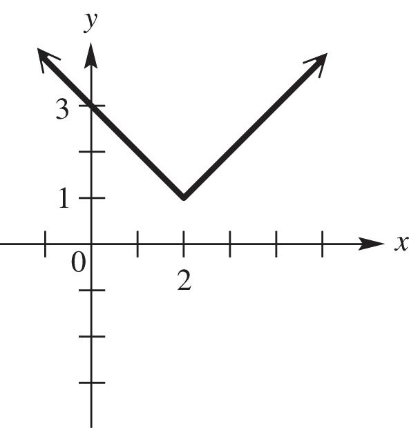
Figure 29
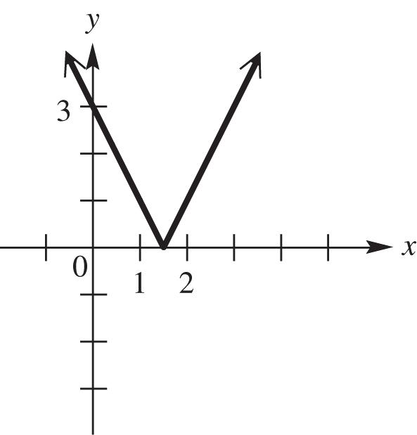
Figure 30
31. (a) From the graph, the function is continuous for the intervals: ,2,2,1 and 1,
(b) From the graph, the function is increasing for the interval: 2,1
(c) From the graph, the function is decreasing for the interval: ,2
(d) From the graph, the function is constant for the interval: 1,
(e) From the graph, all values can be input for x, therefore the domain is: ,
(f) From the graph, the possible values of y or the range is:
32. 22444xyyxyx and 4 yx .
21,12,
33. From the graph, the relation is symmetric with respect to the x-axis, y-axis, and origin. The relation is not a function since some inputs x have two outputs y.
34. If 3 6 Fxx ,then 3 3 66FxxFxx
and
3366FxxFxx
. Since FxFxFx the function has no symmetry and is neither an ever nor an odd function.
35. If ||4fxx ,then ||4||4fxxfxx
and ||4fxx Since fxfx the function is symmetric with respect to the y-axis and is an even function.
36. If 5 fxx then 5 fxx and 5 fxx .Since fxfxfx , the function has no symmetry and is neither an even nor an odd function.
37. If 2 5 yx then 5 yx . Since 5 fxx is the reflection of 5 fxx across the x-axis, the relation has symmetry with respect to the x-axis. Also, one x inputs can produce two y outputs the relation is not a function.
38. If 42 321fxxx then 42 42 321321 fxxxfxxx
and 42 321fxxx Since fxfx the function is symmetric with respect to the y-axis and is an even function.
39. True, a graph that is symmetrical with respect to the x-axis means that for every , xy there is also , xy
40. True, since an even function and one that is symmetric with respect to the y-axis both contain the points , xy and , xy .
41. True, since an odd function and one that is symmetric with respect to the origin both contain the points , xy and , xy
42. False, for an even function, if , ab is on the graph, then , ab is on the graph and not , ab . For example, 2 fxx is even, and (2, 4) is on the graph, but (2, 4) is not.
43. False, for an odd function, if , ab is on the graph, then , ab is on the graph and not , ab For example, 3 fxx is odd, and 2,8 is on the graph, but 2,8 is not.
44. True, if ,0x is on the graph of 0 fx then ,0x is on the graph.
45. The graph of 2 348yx is the graph of 2 yx shifted 4 units to the left, vertically stretched by a factor of 3, reflected across the x-axis, and shifted 8 units downward.
46. The equation yx reflected across the y-axis is: () fxx then reflected across the x-axis is: yx now vertically shrunk by a factor of 2 3 is: 2 3 yx , and finally shifted 4 units upward is: 2 4 3 yx .
47. Shift the function f upward 3 units. See Figure 47.
Copyright © 2019 Pearson Education, Inc.
48. Shift the function f to the right 2 units. See Figure 48.
49. Shift the function f to the left 3 units and downward 2 units. See Figure 49.
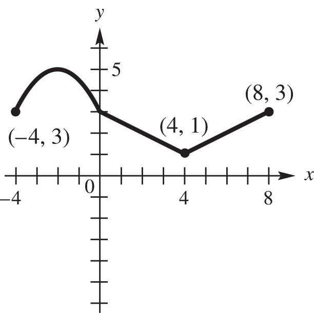
Figure 47
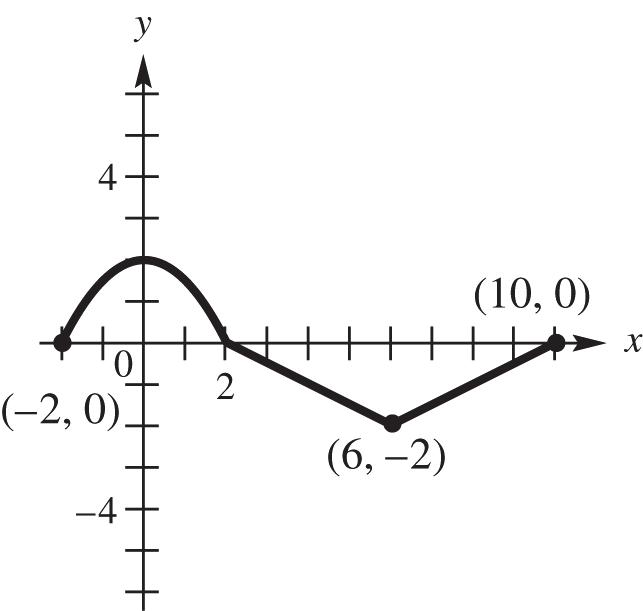
Figure 48
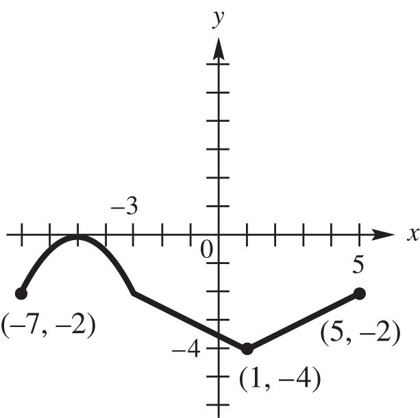
49
50. For values where 0 fx the graph remains the same. For values where 0 fx reflect the graph across the x-axis. See Figure 50.
51. Horizontally shrink the function f by a factor of 1 4 . See Figure 51.
52. Horizontally stretch the function f by a factor of 2. See Figure 52.
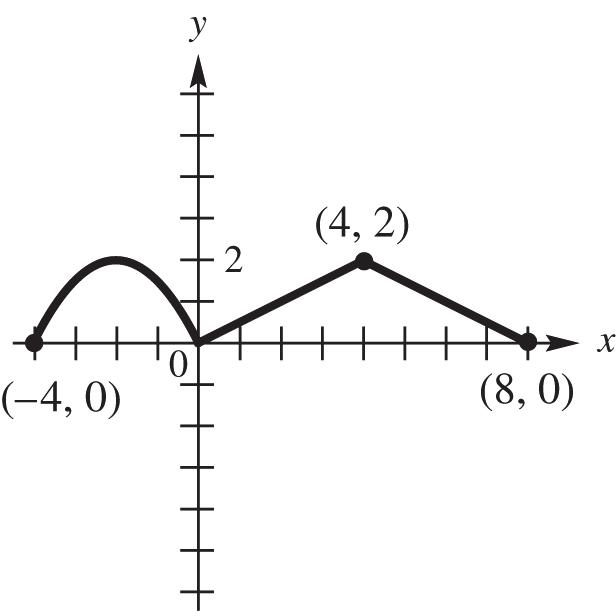
Figure 50

Figure 51
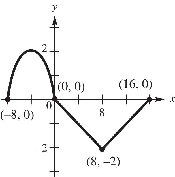
Figure 52
53. The function is shifted upward 4 units, therefore the domain remains the same: 3,4 and the range is increased by 4 and is: 2,9
54. The function is shifted left 10 units, therefore the domain is decreased by 10 and is 13,6; and the function is stretched vertically by a factor of 5, therefore the range is multiplied by 5 and is: 10,25.
55. The function is horizontally shrunk by a factor of 1 , 2 therefore the domain is divided by 2 and is: 3 ,2; 2
and the function is reflected across the x-axis, therefore the range is opposites of the original and is:
5,2.
56. The function is shifted right 1 unit, therefore the domain is increased by 1 and is: 2,5; and the function is also shifted upward 3 units, therefore the range is increased by 3 and is: 1,8.
57. We reflect the graph of yfx across the x-axis for all points for which 0. y Where 0, y the graph remains unchanged. See Figure 57.
58. We reflect the graph of yfx across the x-axis for all points for which 0. Where 0, y the graph remains unchanged. See Figure 58.
59. Since the range is 2,0, y so the graph remains unchanged.
60. Since the range is 2,0, y so we reflect the graph across the x-axis. See Figure 60.
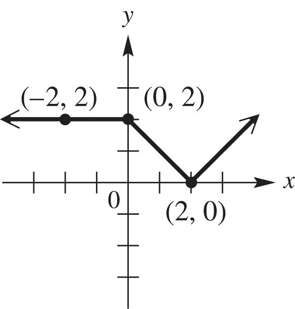


4312431249 4
or 15 4312415, 4 xxx
therefore the solution set
62. 2641263. xx
Since an absolute value equation can not have a solution less than zero, the solution
63. 53115311482
therefore the solution set is: 7 ,2. 3
64. 257257221 xxxx
or 2572126, xxx
63
therefore the solution set is:
65. 2577257122261, xxxx
therefore the interval is:
66. 257257221 xxxx +³+³³³ or 2572126, xxx +£-£-£- therefore the solution is the interval: ( ] [ ) ,61,.-¥-¥
67. 12 51205120512 5 xxxx
or 12 5120512, 5 xxx
therefore the solution is the interval: 1212 ,, 55
68. Since an absolute value equation can not have a solution less than zero, the solution set is:
Copyright © 2019 Pearson Education, Inc.
69. 11 2311212312031103110311 3 xxxxxx or 3110393, xxx
therefore the solution set is: 11 3,. 3
70. 21312131500 xxxxxx or 213122, xxxx therefore the solution set is: 0,2.
71. The x-coordinates of the points of intersection of the graphs are 6 and 1.Thus, 6,1 is the solution set of 12yy The graph of 1y lies on or below the graph of 2y between 6 and 1, so the solution set of 12yy is 6,1 The graph of 1y lies above the graph of 2y everywhere else, so the solution set of 12yy is
72. Graph 1 13yxx and {3,1} See Figure 72. The intersections are 3 x and 5, x therefore the solution set is: 3,5. Check:
3133826826888
and
5153862862888
[-10,10] by [-4,16] Xscl = 1 Yscl = 1

73. Initially, the car is at home. After traveling 30 mph for 1 hr, the car is 30 mi away from home. During the second hour the car travels 20 mph until it is 50 mi away. During the third hour the car travels toward home at 30 mph until it is 20 mi away. During the fourth hour the car travels away from home at 40 mph until it is 60 mi away from home. During the last hour, the car travels 60 mi at 60 mph until it arrives home.
74. See Figure 74
75. See Figure 75
76. See Figure 76

Figure 74
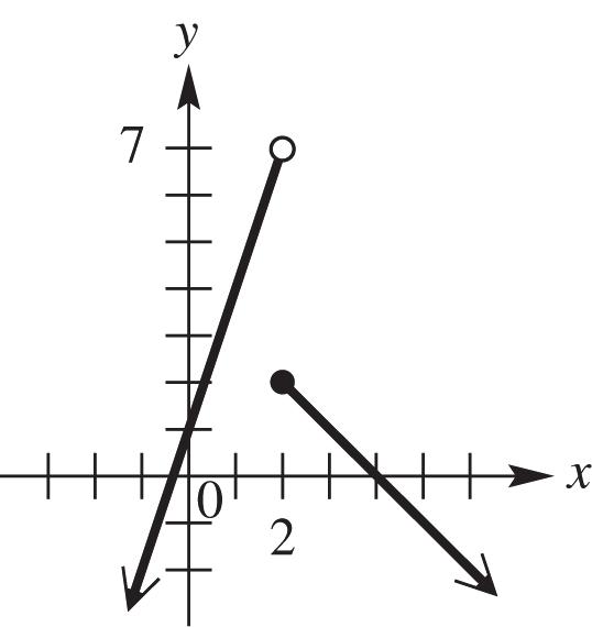
Figure 75
77. Graph 1 31*24*2yxxxx in the window
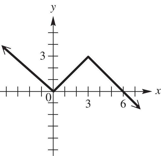
Figure 76
78. See Figure 78.
[-10,10] by [-10,10] [-5,5] by [-5,5] Xscl = 1 Yscl = 1 Xscl = 1 Yscl = 1
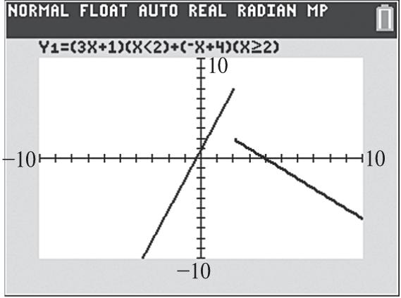

Figure 77 Figure 78
79. From the graphs ()(1)235 fg
80. From the graphs ()(0)143 fg
81. From the graphs ()(1)(0)(3)0 fg
82. From the graphs 3 (2) 2 f g
83. From the graphs ()(2)[(2)](2)3 fgfgf
84. From the graphs ()(2)[(2)](3)2 gfgfg
85. From the graphs ()(4)[(4)](2)2 gfgfg
86. From the graphs ()(2)[(2)](2)3 fgfgf
87. From the table ()(1)718 fg
88. From the table ()(3)910 fg
89. From the table ()(1)(3)(2)6 fg
90. From the table 5 (0) 0 f g , which is undefined.
91. From the tables ()(2)[(2)](1)2 gfgfg
92. From the graphs ()(3)[(3)](2)1 fgfgf
Copyright © 2019 Pearson Education, Inc.
93. 2()9(29)229292 2 xhxxhxh hhh
94. 22222 ()5()3(53)255353 xhxhxxxxhhxhxx hh 2 25 25 xhhh xh h
95. One of many possible solutions for ()()() fgxhx is: 2 () fxx and 3 ()3 gxxx Then 2 3 ()3 fgxxx
96. One of many possible solutions for ()()() fgxhx is 1 ()fx x and ()5gxx Then 1 ()()[()] 5 fgxfgx x
97. If 3 4 () 3 Vrr , then a 4 inch increase would be: 3 4 ()(4) 3 Vrr , and the volume gained would be: ()(4)4433 33 Vrrr
98. (a) Since , 2 d hdr and the formula for the volume of a can is: 2 Vrh , the function is: 2 3 ()()24 dd VddVd
(b) Since ,,2 2 d hdrcr and the formula for the surface area of a can is: 2 22 Arhr , the function is: 2 22 2 3 ()22()()2222 dddd SddSddSd
99. The function for changing yards to inches is: ()36 fxx and the function for changing miles to yards is: ()1760 gxx The composition of this which would change miles into inches is: [()]36[1760()]()()63,360 fgxxfgxx .
100. If x width, then length 2 x A formula for Perimeter can now be written as: 22 Pxxxx and the function is: ()6 Pxx This is a linear function.
Chapter 2 Test
1. (a) D, only values where 0 x can be input into a square root function.
(b) D, only values where 0 y can be the solution to a square root function.
(c) C, all values can be input for x in a squaring function.
(d) B, only values where 3 y can be the solution to 2 ()3fxx
(e) C, all values can be input for x in a cube root function.
(f) C, all values can be a solution in a cube root function.
(g) C, all values can be input for x in an absolute value function.
(h) D, only values where 0 y can be the solution to an absolute value function.
(i) D, if 2 xy then yx and only values where 0 x can be input into a square root function.
(j) C, all values can be a solution in this function.
2. (a) This is ()fx shifted 2 units upward. See Figure 2a.
(b) This is ()fx shifted 2 units to the left. See Figure 2b.
(c) This is ()fx reflected across the x-axis. See Figure 2c.
(d) This is ()fx reflected across the y-axis. See Figure 2d.
(e) This is ()fx vertically stretched by a factor of 2 . See Figure 2e.
(f) We reflect the graph of ()yfx across the x-axis for all points for which $2.75 Where 0 y the graph remains unchanged. See Figure 2f.
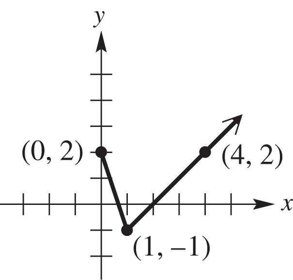
Figure 2a

Figure 2d
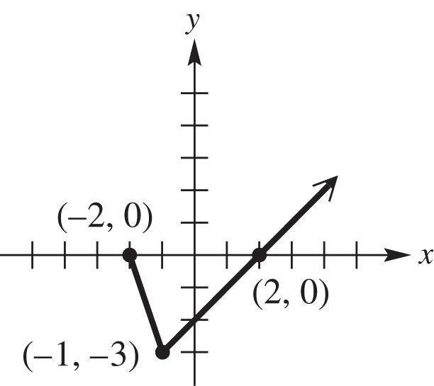
Figure 2b
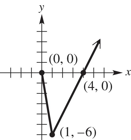
Figure 2e
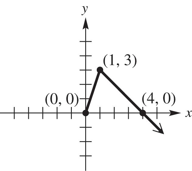
Figure 2c

Figure 2f
3. (a) Since (2)yfx is ()yfx horizontally shrunk by a factor of 1 2 , the point (2,4) on ()yfx becomes the point (1,4) on the graph of (2)yfx .
(b) Since 1 2 yfx
is ()yfx horizontally stretched by a factor of 2, the point (2,4) on ()yfx becomes the point (4,4) on the graph of 1 2 yfx
4. (a) The graph of 2 ()(2)4fxxx is the basic graph 2 () fxx reflected across the x-axis, shifted 2 units to the right, and shifted 4 units upward. See Figure 4a.
(b) The graph of ()2 fxx is the basic graph () fxx reflected across the y-axis and vertically stretched by a factor of 2 . See Figure 4b.
Copyright © 2019 Pearson Education, Inc.
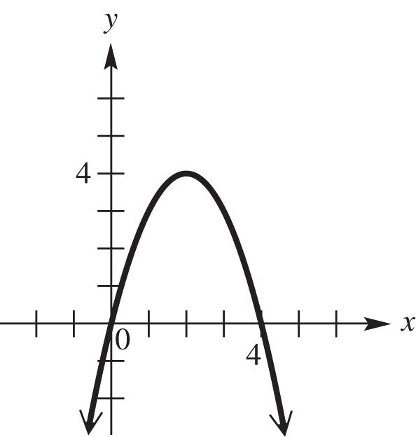
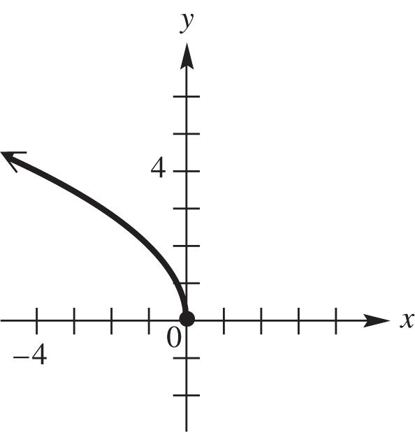
5. (a) If the graph is symmetric with respect to the y-axis, then (,)(,) xyxy therefore (3,6)(3,6)
(b) If the graph is symmetric with respect to the x-axis, then (,)(,) xyxy therefore (3,6)(3,6) .
(c) See Figure 5. We give an actual screen here. The drawing should resemble it.
= 1 Yscl = 1
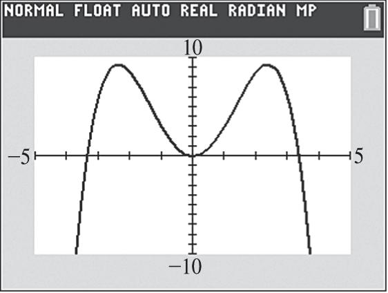
5
6. (a) Shift the graph of 3 yx to the left 2 units, vertically stretch by a factor of 4 , and shift 5 units downward.
(b) Graph yx reflected across the x-axis, vertically shrunk by a factor of 1 2 shifted 3 units to the right, and shifted up 2 units. See Figure 6. From the graph the domain is: (,) ; and the range is: (,2] .
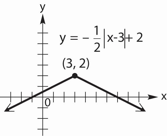
6
7. (a) From the graph, the function is increasing for the interval: (,3)
(b) From the graph, the function is decreasing for the interval: (4,)
(c) From the graph, the function is constant for the interval: 3,4
(d) From the graph, the function is continuous for the intervals: (,3),3,4,(4,) .
(e) From the graph, the domain is: (,)
(f) From the graph, the range is: (,2)
Copyright © 2019 Pearson Education, Inc.
8. (a) 484484441 xxxx
or 4844123 xxx
, therefore the solution set is: {3,1}
(b) 4844484124431 xxxx
, therefore the solution is: (3,1) .
9.
(c) 484484441 xxxx
or 4844123 xxx
therefore the solution is: (,3)(1,) .
(b) 2 232 () 21 fxx x gx
(c) The domain can be all values for x, except any that make ()gx =0. Therefore 1
(d) 22 ()()2(21)3(21)22(441)632 fgxfgxxxxxx
-++-+=-+
(e) 222 ()()2(232)14641463 gfxgfxxxxxxx
(f) 22222 2()3()2(232)2(2)332232 xhxhxxxxhhxhxx hh 2222 242332232423 423 xxhhxhxxxhhh xh
10. (a) ()()[()]211 fgxfgxx D:
(b) (g)()[f()]2112 fxgxxx
11. (a) See Figure 11a.
(b) Graph
See Figure 11b.
(c) The graph is not connected at x = 1 and thus f is not continuous when x =1.
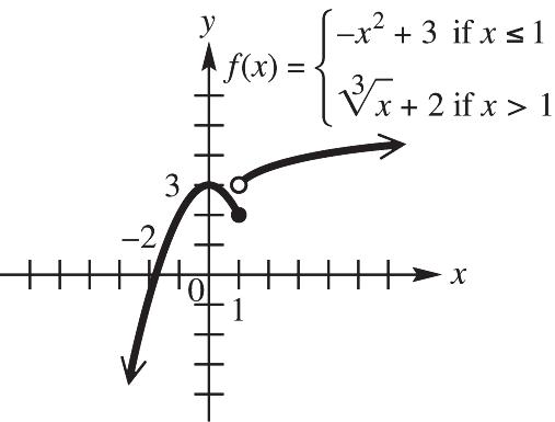
Figure 11a
Copyright © 2019 Pearson Education, Inc.
[-4.7,4.7] by [-5.1,5.1]
[0,10] by [0,6]
Section 2.T 151
[0,1,000] by [-4,000,4000]
Xscl = 1 Yscl = 1 Xscl = 1 Yscl = 1 Xscl = 50 Yscl = 500
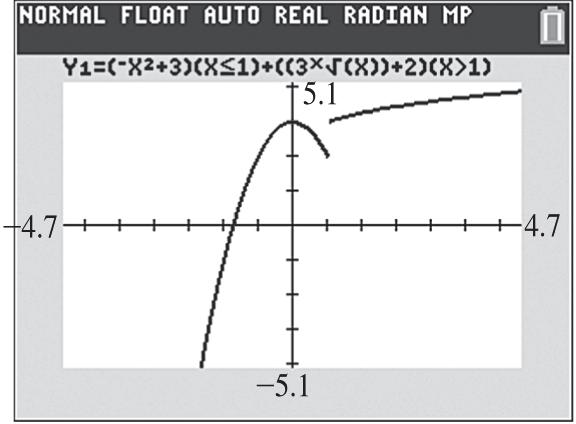
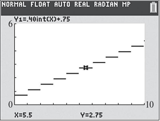

12. (a) See Figure 12.
(b) Set 5.5 x then $2.75 is the cost of a 5.5 minute international call. See the display at the bottom of the screen.
13. (a) With an initial set-up cost of $3300 and a production cost of $4.50 the function is: ()33004.50 Cxx
(b) With a selling price of $10.50 the revenue function is: ()10.50 Rxx
(c) ()()()()10.50(33004.50)()63300 PxRxCxPxxxPxx
(d) To make a profit ()0,Px therefore 63300063300550 xxx Tyler needs to sell 551 before he earns a profit.
(e) Graph 1 63300,yx See Figure 13. The first integer x-value for which ()0Px is 551
Copyright © 2019 Pearson Education, Inc.
