Solutions for Differential Equations And Linear Algebra 2nd Us Edition by Farlow by 6alsm

Linearity and Nonlinearity

2.1 Linear Equations: The Nature of Their Solutions

Classification

1. First-order, nonlinear

2. First-order, linear, nonhomogeneous, variable coefficients

3. Second-order, linear, homogeneous, variable coefficients

4. Second-order, linear, nonhomogeneous, variable coefficients

5. Third-order, linear, homogeneous, constant coefficients

6. Third-order, linear, nonhomogeneous, constant coefficients

7. Second-order, linear, nonhomogeneous, variable coefficients

8. Second-order, nonlinear

9. Second-order, linear, homogeneous, variable coefficients

10. Second-order, nonlinear

Linear Operation Notation

11. Using the common differential operator notation that D(y) = dy dt , we have the following:

(a) 30ytyy′′′+−= can be written as L(y) = 0 for L = D2 + tD 3.

(b) y ′ + y 2 = 0 is not a linear DE.

(d) y ′ + t2 y = 0 can be written as L(y) = 0 for L = D + t2

SECTION 2.1 Linear Equations: The Nature of Their Solutions 93

(e) y ′ + (sin t)y = 1 can be written as L(y) = 1 for L = D + sin t

(f) 3 yyy ′′′−+ = sin t can be written as L(y) = sin t for L = D2 3D + 1.

Linear and Nonlinear Operations

12. ( ) 2 Lyyy ′ =+

Suppose 12 , yy and y are functions of t and c is any constant. Then ()()()

Hence, L is a linear operator.

13. ( ) 2 Lyyy ′ =+

To show that ( ) 2 Lyyy ′ =+ is not linear we can pick a likely function of t and show that it does not satisfy one of the properties of linearity, equations (2) or (3). Consider the function yt = and the constant 5 c = :

Hence, L is not a linear operator.

14. ( ) 2 Lyyty ′ =+

Suppose 12 , yy and y are functions and c is any constant. ()()()

Hence, L is a linear operator. This problem illustrates the fact that the coefficients of a DE can be functions of t and the operator will still be linear.

15. ( ) t Lyyey ′ =−

Suppose 12 , yy and y are functions of t and c is any constant.

Hence, L is a linear operator. This problem illustrates the fact that a linear operator need not have coefficients that are linear functions of t

16. ( ) ( ) sin Lyyty ′′ =+

Hence, L is a linear operator. This problem illustrates the fact that a linear operator need not have coefficients that are linear functions of t.

17. ( ) ( ) 2 1 Lyyyyy ′′′ =+−+

Hence, ( ) Ly is not a linear operator.

Pop Quiz

() 2 1 21

SECTION 2.1 Linear Equations: The Nature of Their Solutions 95

22. 51yy ′ += , ()() 5 1 10 5 yytcet=⇒=+ , () 5 1 10 5 yce =⇒=− . Hence, () () () 51 1 1 5 ytet =−

23. 24yy ′ += , ( ) ( ) 2 012yytcet=⇒=+ , ( ) 011yc = ⇒=− . Hence, () 2 2 ytet =−

Superposition Principle

24. If 1y and 2y are solutions of ( ) 0 ypty ′ + = , then ( ) () 11 22 0 0. ypty ypty ′ + = ′ + =

Adding these equations gives ( ) ( ) 1212 0 yyptypty ′′ + ++= or ()()() 1212 0 yyptyy ′ + ++= , which shows that 12yy + is also a solution of the given equation. If 1y is a solution, we have ( ) 11 0 ypty ′ + = and multiplying by c we get ( ) ( ) () ()()() 11 11 11 0 0 0, cypty cycpty cyptcy ′ + = ′ + = ′ + = which shows that 1cy is also a solution of the equation.

Second-Order Superposition Principle

25. If 1y and 2y are solutions of ( ) ( ) 0 yptyqty ′′′ + += , we have ( ) ( ) ()() 111 222 0 0. yptyqty yptyqty ′′′ + += ′′′ + +=

Multiplying these equations by 1c and 2c respectively, then adding and using properties of the derivative, we arrive at ()()()()() 112211221122 0 cycyptcycyqtcycy ′′′ +++++= , which shows that 1122 cycy + is also a solution.

Verifying Superposition

26. 90;yy ′′ −= 3 1 t ye = ⇒ 3 1 3 t ye ′ = ⇒ 3 1 9, t ye ′′ = so that 33 119990 tt yyee ′′ =−= 3 2 t ye = ⇒ 3 2 3 t ye ′ =− ⇒ 3 2 9, t ye ′′ = so that 33 229990 tt yyee ′′ =−= .

Let y3 = c1y1 + c2y2 = c1e 3t + c2e 3t , then 333123(3)tt ycece ′ =+− 3331299tt ycece ′′ =+

Thus, 3333 331212 9(99)9()0 tttt yycececece ′′ −=+−+=

27. 40;yy ′′ +=

For y1 = sin 2t, 1 2cos2 yt ′ = ⇒ 1 4sin2,yt ′′ = so that 1144sin24sin20 yytt ′′ + =−+= .

For y2 = cos 2t, 2 2sin2 yt ′ =− ⇒ 2 4cos2, yt ′′ = so that 2244cos24cos20 yytt ′′ + =−+= .

Let y3 = c1 sin 2t + c2 cos 2t, then 3122cos2(2sin2) yctct ′ = +− 312(4sin2)(4cos2) yctct ′′ = −+−

Thus, 331212 4(4sin2)(4cos2)4(sin2cos2)0 yyctctctct ′′ +=−+−++= .

28. 20; yyy′′′+−=

For y1 = e t/2 , /2 1 1 2 t ye ′ = , /2 1 1 4 t ye ′′ = .

Substituting: 11/2/2/2 20 42 ttt eee ⎛⎞ +−= ⎜⎟ ⎝⎠ .

For y2 = e t , 2 , t ye ′ =− 2 t ye ′′ =

Substituting: ( ) ( ) 2 ttt eee +−− = 0.

For c1 and c2, let y = c1e t/2 + c2e t

Substituting: ()/2/2/2 121212 11 2 42 tttttt cececececece ⎛⎞⎛⎞ ⎜⎟⎜⎟++−−+ ⎝⎠⎝⎠ = 0.

SECTION 2.1 Linear Equations: The Nature of Their Solutions

29. 560yyy ′′′−+=

For y1 = e 2t , 2 1 2 t ye ′ = , 2 1 4 t ye ′′ =

Substituting: 222 45(2)6()0 ttt eee−+= .

For y2 = e 3t , 3 2 3, t ye ′ = 3 2 9 t ye ′′ = .

Substituting: 333 95(3)60 ttt eee−+=

For y = c1e 2t + c2e 3t , ( ) ( ) 232323 121212 564952360 tttttt yyycececececece ′′′−+=+−+++=

30. 60yyy ′′′ −−=

For y1 = e 3t , 3 1 3, t ye ′ = 3 1 9 t ye ′′ =

Substituting: 33)3 (9)(3)6()0 ttt eee−−=

For y2 = e 2t , 2 2 2, t ye ′ =− 2 2 4 t ye ′′ =

Substituting: 222 (4)(2)60 ttt eee−−−=

For y = c1e 3t + c2e 3t ( ) ( ) ( ) 323233 12112 6943260 tttttt yyycececeecece ′′′−−=+−−−+=

31. 90yy ′′ −=

For y1 = cosh 3t, 1 3sinh3 yt ′ = 1 9cosh3 yt ′′ = .

Substituting: (9cosh3)9(cosh3)0 tt−=

For y2 = sinh 3t, 2 3cosh3, yt ′ = 2 9sinh3 yt ′′ = .

Substituting: (9sinh3)9(sinh3) tt = 0.

For y = c1 cosh 3t + c2 sinh 3t, ( ) ( ) 1212 99cosh39sinh39cosh3sinh30 yyctctctct ′′ −=+−+=

2 Linearity and Nonlinearity

Different Results?

32. The solutions of Problem 31, cosh 3t = 333 2 tt e + and sinh 3t = 33 2 tt ee , are linear combinations of the solutions of Problem 26 and vice-versa, i.e., e 3t = cosh 3t + sinh 3t and e 3t = cosh 3t sinh 3t.

Many from One

33. Because ( ) 2 ytt = is a solution of a linear homogeneous equation, we know by equation (3) that 2 ct is also a solution for any real number c

Guessing Solutions

We can often find a particular solution of a nonhomogeneous DE by inspection (guessing). For the firstorder equations given for Problems 27–31 the general solutions come in two parts: solutions to the associated homogeneous equation (which could be found by separation of variables) plus a particular solution of the nonhomogeneous equation. For second-order linear equations as Problems 32–35 we can also sometimes find solutions by inspection.

34. () 1 2 ttt yyeytcee ′ +=⇒=+

36. ( ) ttt yyeytcete ′ −=⇒=+

38. () 4 3 5 yctytyt tt ′ +=⇒=+

( ) ttt yyeytcete ′ +=⇒=+

39. ( ) 2 12 0 atatyayytcece ′′ −=⇒=+ . An alternative form is ( ) ( ) ( ) 12 sinhcosh ytcatcat =+ .

40. ( ) 2 12 0sincos yayytcatcat ′′ +=⇒=+ 41. ( ) 12 0 yyytccet ′′′+=⇒=+

42. ( ) 12 0 tyyytcce ′′′−=⇒=+

Nonhomogeneous Principle

In these problems, the verification of p y is a straightforward substitution. To find the rest of the solution we simply add to p y all the homogeneous solutions hy , which we find by inspection or separation of variables.

43. 3 t yye ′ −= has general solution ()3tt hp ytyycete =+=+ .

44. 210sin yyt ′ += has general solution ( ) 2 4sin2cos t hp ytyycett =+=+− .

45. 2 2 yyy t ′ −= has general solution ( ) 23 hp ytyyctt = +=+ .

46. 1 2 1 yy t ′ += + has general solution () 2 2 11 hp ctt ytyy tt + =+=+ + + .

Third-Order Examples

47. (a) For y1 = e t, we substitute into 0 yyyy ′′′′′′−−+= to obtain e t e

For y2 = tet, we obtain 2 , ttytee ′ = + 2 (), ttt yteee ′′ = ++ 2 ()2, ttt yteee ′′′ =++ and substitute to verify (tet + 3e t) (tet + 2et) (tet + e t) + tet = 0. For y3 = e t, we obtain 333,,, ttt yeyeye ′′′′′′ =−==− and substitute to verify

Given

: 2 22 t p ye ′ =+ 2 4 t p ye ′′ = 2 8 t p ye ′′′ =

verify:

100 CHAPTER 2 Linearity and Nonlinearity (e)

(0) y ′ = 2

Equation (1)

Equation (2) (0) y ′′ = 3

Add Equation (2) to (1) and (3)

12 12 23 233 cc cc +=− ⎫ ⎬ +=− ⎭ ⇒

Thus, y = 2 31 21. 22 ttt eete −++++

48. 4sin3yyyyt ′′′′′′+−−=+

(a) For y1 = e t, we obtain by substitution 0 tttt yyyyeeee ′′′′′′+−−=+−−=

For y = e t, we obtain by substitution

()()0tttt yyyyeeee ′′′′′′+−−=−+−−−=

For y = tet we obtain by substitution

Equation (3)

(3)(2)()0 ttttttt yyyyteeteeteete ′′′′′′+−−=−++−−−+−= .

(b) yh = c1e t + c2e t + c3tet

To verify:

(sincos)(cossin)(sincos)(cossin3) 4sin3 pppp yyyytttttttt t ′′′′′′+−−=++−+−−−−−− =+

(d) y(t) = yh + yp = c1e t + c2e t + c3tet + cos t sin t 3

SECTION 2.1 Linear Equations: The Nature of Their Solutions 101

Add Equation (2) to (1) and (3)

Suggested Journal Entry

49. Student Project

Equation (1)

Equation (2)

Equation (3)

2.2 Solving the First-Order Linear Differential Equation

General Solutions

The solutions for Problems 1–15 can be found using either the Euler-Lagrange method or the integrating factor method. For problems where we find a particular solution by inspection (Problems 2, 6, 7) we use the Euler-Lagrange method. For the other problems we find it more convenient to use the integrating factor method, which gives both the homogeneous solutions and a particular solution in one swoop. You can use the Euler-Lagrange method to get the same results.

1. 20yy ′ +=

By inspection we have ( ) 2 ytcet =

2. 23 t yye ′ +=

We find the homogeneous solution by inspection as 2 t h yce = . A particular solution on the nonhomogeneous equation can also be found by inspection, and we see t p ye = . Hence the general solution is ( ) 2 ttytcee =+

3. 3 t yye ′ −=

We multiply each side of the equation by the integrating factor () ()() 1 ptdtdtt teee μ ∫∫ === giving ( ) 3 t eyy ′ −= , or simply () 3 dt dtye = .

Integrating, we find 3 t yetc =+ , or ( ) 3 tt ytcete =+ .

4. sin yyt ′ +=

We multiply each side of the equation by the integrating factor ( ) t te μ = , giving () sin tt eyyet ′ += , or, () sin dtt dtyeet = .

Integrating by parts, we get () 1 sincos 2 tt yeettc =−+ .

Solving for y, we find () 11 sincos 22 t ytcett =+−

5. 1 1 yyt e ′ += +

We multiply each side of the equation by the integrating factor ( ) t te μ = , giving

Integrating, we get ( ) ln1 tt yeec =++

Hence, () ( ) ln1 ttt ytceee =++ .

6. 2 ytyt ′ +=

In this problem we see that () 1 2 p yt = is a solution of the nonhomogeneous equation (there are other single solutions, but this is the easiest to find). Hence, to find the general solution we solve the corresponding homogeneous equation, 20yty ′ + = , by separation of variables, getting 2 dytdt y =− , which has the general solution 2 t yce = , where c is any constant.

Adding the solutions of the homogeneous equation to the particular solution 1 2 p y = we get the general solution of the nonhomogeneous equation:

7. 22 3 ytyt ′ +=

In this problem we see that () 1 3 p yt = is a solution of the nonhomogeneous equation (there are other single solutions, but this is the easiest to find). Hence, to find the general solution, we solve the corresponding homogeneous equation, 2 30yty ′ + = , by separation of variables, getting 2 3 dytdt y =− , which has the general solution () 3 ytcet = , where c is any constant. Adding the solutions of the homogeneous equation to the particular solution

p y = , we get the general solution of the nonhomogeneous equation

104 CHAPTER 2 Linearity and Nonlinearity

8. 2 11 yy tt ′ += , ( ) 0 t ≠

We multiply each side of the equation by the integrating factor () ln dttt teet μ ∫ = == , giving () 111 , or, . d tyytyttdtt ⎛⎞ ′ + == ⎜⎟ ⎝⎠

Integrating, we find ln tytc =+

Solving for y, we get () 1 ln c ytt tt

9. 2 tyyt ′ +=

We rewrite the equation as 1 2 yy t ′ += , and multiply each side of the equation by the integrating factor () ln dttt teet μ ∫ === , giving () 1 2, or, 2. d tyyttyt tdt

Integrating, we find 2 tytc =+

Solving for y, we get () c ytt t =+ .

10. ( ) cossin1 tyty ′ +=

We rewrite the equation as ( ) tansec ytyt ′ += , and multiply each side of the equation by the integrating factor () ()() 1 lncoslncos tan sec tdttt teeet μ ∫ ==== , giving () () () () sectansec,22 or, secsec. d tytyttyt dt ′ +==

Integrating, we find ( ) sectantytc =+ . Solving for y, we get ( ) cossin ytctt =+

SECTION 2.2 Solving the First-Order Linear Differential Equation

11. 2 2 cos yytt t ′ −= , ( ) 0 t ≠

We multiply each side of the equation by the integrating factor () () 2 2 2lnln2tdttt teeet μ ∫ ==== , giving

22 2 cos, or, cos. d tyyttyt tdt

Integrating, we find 2 sin tytc =+ . Solving for y, we get ( ) 22 sin ytcttt =+ .

12. 3 3sin t yy tt ′ += , ( ) 0 t ≠

We multiply each side of the equation by the integrating factor () () ( ) 3 ln 3 3ln3tdtt t teeet μ ∫ = === , giving

33 3 sin, or, sin. d tyyttyt tdt

Integrating, we find 3 cos tytc =−+ .

Solving for y, we get () 33 1 cos c ytt tt =− .

13. ( ) 10 tt eyey ′ ++=

We rewrite the equation as 0 1 t t e yy e

′ + = ⎜⎟ + ⎝⎠ , and then multiply each side of the equation by the integrating factor () ( ) ( ) 1ln1 1 ttt eedtet teee μ ++ ∫ = ==+ , giving () ( ) 10dt dtey + =

Integrating, we find ( ) 1 t eyc+= . Solving for y, we have () 1 t c yt e = + .

14. ( ) 2 90tyty ′ ++=

We rewrite the equation as 2 0 9 t yy t ⎛⎞ ′ += ⎜⎟ + ⎝⎠ , and then multiply each side of the equation by the integrating factor

, giving ( ) 2 90 d dtty+=

Integrating, we find 2 9 tyc += .

Solving for y, we find ()

yt t = +

15. 21 2 t yyt t + ⎛⎞ ′ += ⎜⎟ ⎝⎠ , ( ) 0 t ≠

We multiply each side of the equation by the integrating factor

, giving

Integrating, we find

Solving for y, we have

Initial-Value Problems

16. 1 yy ′ −= , ( ) 01 y =

By inspection, the homogeneous solutions are t h yce = . A particular solution of the nonhomogeneous can also be found by inspection to be 1 p y = . Hence, the general solution is

t hp yyyce = +=− .

Substituting ( ) 01 y = gives 11 c −= or 2 c = . Hence, the solution of the IVP is ( ) 21 t yte =

SECTION 2.2 Solving the First-Order Linear Differential Equation 107

17. 3 2 ytyt ′ += , ( ) 11 y =

We can solve the differential equation using either the Euler-Lagrange method or the integrating factor method to get

2 2 11 22 yttcet =−+ .

Substituting ( ) 11 y = we find 1 1 ce = or c = e. Hence, the solution of the IVP is () 2 1121 22 yttet =−+ .

18. 3 3 yyt t ⎛⎞ ′ −= ⎜⎟

, ( ) 14 y =

We find the integrating factor to be

Multiplying the DE by this, we get

3 1 d dtty =

Hence, 3 tytc =+ , or, 34 () ytctt = +

Substituting ( ) 14 y = gives 14 c + = or 3 c = . Hence, the solution of the IVP is ( ) 34 3 yttt = + .

19. 2 ytyt ′ += , ( ) 01 y =

We solved this differential equation in Problem 6 using the integrating factor method and found () 2 1 2 ytcet = +

Substituting ( ) 01 y = gives 1 1 2 c + = or 1 2 c = . Hence, the solution of the IVP is () 2 11 22ytet = +

20. ( ) 10 tt eyey ′ ++= , ( ) 01 y =

We solved this DE in Problem 13 and found () 1 t c yt e = +

Substituting ( ) 01 y = gives 1 2 c = or 2 c = . Hence, the solution of the IVP is () 2 1 ytt e = +

Synthesizing Facts

21. (a) () () 2 2 , 1 1 tt ytt t + =>− +

(b) ( ) ( ) 1, 1 yttt=+>−

Hence, when 1 t ≠− we have 1 yt = + .

(d) The solution passing through the origin ( ) 0, 0 asymptotically approaches the line 1 yt=+ as t →∞ , which is the solution passing through ( ) 01 y = . The entire line 1 yt=+ is not a solution of the DE, as the slope is not defined when 1 t =− . The segment of the line 1 yt=+ for 1 t >− is the solution passing through ( ) 01 y = .

On the other hand, if the initial condition were ( ) 54 y =− , then the solution would be the segment of the line 1 yt = + for t less than –1. Notice in the direction field the slope element is not defined at ( ) 1, 0 .

Using Integrating Factors

In each of the following equations, we first write in the form ( ) ( ) yptyft ′ += and then identify ( ) pt

22. 20yy ′ +=

Here ( ) 2 pt = , therefore the integrating factor is ()

= ==

Multiplying each side of the equation 20yy ′ + = by 2 t e yields

Integrating gives 2 t yec = . Solving for y gives ( ) 2 ytcet =

23. 23 t yye ′ +=

Here ( ) 2 pt = , therefore the integrating factor is ()

2 2 ptdtdtt teee μ

= ==

Multiplying each side of the equation 23 t yye ′ += by 2 t e yields

23 3 dtt dtyee =

Integrating gives 23 tt yeec =+ . Solving for y gives ( ) 2 ttytcee = +

SECTION 2.2 Solving the First-Order Linear Differential Equation

24. 3t yye ′ −=

Here ( ) 1 pt =− , therefore the integrating factor is () () ptdtdtt teee μ ∫∫ ===

Multiplying each side of the equation 3t yye ′ = by t e yields () 2 dtt dtyee = .

Integrating gives 2 1 2 tt yeec =+ . Solving for y gives () 3 1 2 ttytcee =+ .

25. sin yyt ′ +=

Here ( ) 1 pt = therefore the integrating factor is () () ptdtdtt teee μ ∫∫ = == .

Multiplying each side of the equation sin yyt ′ + = by t e gives () sin dtt dtyeet =

Integrating gives () 1 sincos 2 tt yeettc =−+ . Solving for y gives () () 1 sincos 2 ytttcet =−+

26. 1 1 yyt e ′ += +

Here ( ) 1 pt = therefore the integrating factor is () () ptdtdtt teee μ ∫∫ = == .

Multiplying each side of the equation 1 1 yyt e ′ += + by t e yields () 1 t t t de dtyee = +

Integrating gives ( ) ln1 tt yeec =++ . Solving for y gives () ( ) ln1 ttt yteece =++ .

27. 2 ytyt ′ +=

Here ( ) 2 ptt = , therefore the integrating factor is () () 2 2 ptdttdtt teee μ ∫∫ = == .

Multiplying each side of the equation 2 ytyt ′ + = by 2 t e yields ( ) 22dtt dtyete = .

Integrating gives 22 1 2 tt yeec =+ . Solving for y gives () 2 1 2 ytcet = +

110 CHAPTER 2 Linearity and Nonlinearity

28. 22 3 ytyt ′ +=

Here () 2 3 ptt = , therefore the integrating factor is () () 2 3 3 ptdttdtt teee μ ∫∫ === .

Multiplying each side of the equation 22 3 ytyt ′ + = by 3 t e yields ( ) 33 2 dtt dtyete = .

Integrating gives 33 1 3 tt yeec =+ . Solving for y gives () 3 1 3 ytcet = + .

29. 2 11 yy tt ′ +=

Here () 1 pt t = , therefore the integrating factor is () () () 1 ln ptdttdtt teeet μ ∫∫ = ===

Multiplying each side of the equation 2 11 yy tt ′ + = by t yields () 1 d ty dtt =

Integrating gives ln tytc =+ . Solving for y gives () 11 ln ytct tt =+

30. 2 tyyt ′ +=

Here () 1 pt t = , therefore the integrating factor is () () () 1 ln ptdttdtt teeet μ ∫∫ = ===

Multiplying each side of the equation 2 y y t ′ + = by t yields () 2 d dttyt = .

Integrating gives 2 tytc =+ . Solving for y gives () 1 ytct t = +

Switch for Linearity 1 dy dtty = + , ( ) 10 y =

31. Flipping both sides of the equation yields the equivalent linear form dt dyty = + , or dt dyty −=

Solving this equation we get ( ) 1 y tycey=−−

Using the condition ( ) 10 y −= , we find 0 11 ce =− , and so 0 c = . Thus, we have 1 ty=−− and solving for y gives ( ) 1 ytt =

SECTION 2.2 Solving the First-Order Linear Differential Equation 111

The Tough Made Easy 2 2 y dyy dtety =

32. We flip both sides of the equation, getting 2 2 , y dtety dyy = or, 2 2 dtey t dyyy +=

We solve this linear DE for ( ) ty getting () 2 y ec ty y + = .

A Useful Transformation

33. (a) Letting ln zy = , we have z ye = and z dydz e dtdt =

Now the equation ln dyaybyy dt += can be rewritten as zzz dz eaebze dt += .

Dividing by z e gives the simple linear equation dzbza dt =− .

Solving yields bta zce b =+ and using ln zy = , the solution becomes () () btyteabce + = .

(b) If 1 ab== , we have () ( ) 1 t ce yte + = .

Note that when 0 c = we have the constant solution ye = .

Bernoulli Equation ( ) ( ) yptyqtyα ′ += , 0 α ≠ , 1 α ≠

34. (a) We divide by y α to obtain 1 ()() yyptyqt αα ′ += . Let 1 vy α = so that (1) a vyy α ′ ′ =− and 1 va yy α ′ ′ = .

Substituting into the first equation for 1 y α and yy α ′ , we have ()() 1 v ptvqt α ′ += , a linear DE in v, which we can now rewrite into standard form as (1)()(1)() vptvqt α α ′ + −=− .

112 CHAPTER 2 Linearity and Nonlinearity

(b) 3 α = , ( ) 1 pt =− , and ( ) 1 qt = ; hence 22 dv v dt + =− , which has the general solution ( ) 2 1 vtcet =−+

Because 2 1 v y = , this yields () ( ) 12 2 1 ytcet =−+ .

Note, too, that 0 y = satisfies the given equation.

(c) When 0 α = the Bernoulli equation is ()() dy dtptyqt += , which is the general first-order linear equation we solved by the integrating factor method and the Euler-Lagrange method.

When 1 α = the Bernoulli equation is

()() dy dtptyqty += , or, ()() () 0 dyptqty dt + −= , which can be solved by separation of variables.

Bernoulli Practice

35. 3 ytyty ′ += or 32 yytyt ′ +=

Let v = y 2 , so dv dt = 3 2 dy ydt .

Substituting in the DE gives 1 , so that 2 dv tvt dt −+= 22, dv tvt dt =− which is linear in v, with integrating factor μ = 2 2 tdtt ee ∫ =

Thus, 222 22 ttt dv etevte dt −=− , and 222 2,ttt evtedtec = −=+ ∫ so 2 1 t vce =+ .

Substituting back for v gives 2 2 1 , 1 yt ce = + hence 2 1 (). 1 ytt ce =± +

SECTION 2.2 Solving the First-Order Linear Differential Equation 113

36. 2 t yyey ′ −= , so that 21 t yyye ′ =

Let v = y 1 , so 2 dvdy y dtdt =− .

Substituting in the DE gives dvt ve dt + =− , which is linear in v with integrating factor dtt ee μ ∫ =

Thus

Substituting back for

37. 24 23 tytyy ′ −= or 42323ytyty ′ = , t ≠ 0

Let v = y 3 , so 4 3 dvdy y dtdt =− .

Substituting in the DE gives

Thus 654 69 dv ttvt dt +=− , and 645 9 9 5 tvtdttc = −=−+ ∫ , so 5 9 5 vct t =−+ . Substituting back for v gives 3 6 9 5 c y tt =−+ . Hence

38. 22 (1)0 tytyty ′ −−−= (Assume 1 t < )

221 (1) ytytyt ′ −−=

Let v = y 1 , so 2 dvdy y dtdt =−

Substituting in the DE gives 2 (1), dv ttvt dt −−−= so that 22 , 11 dvtt v dttt += which is linear in v, with integrating factor

114 CHAPTER 2 Linearity and Nonlinearity

Thus, 21/223/223/2 (1)(1)(1) dv tttvtt dt −+−=− , and 21/2 23/23/2 1/2 1/221/2 1 (1) 2 (1)

Hence v = 1 + c(1 t2)1/2 and substituting back for v gives y(t) = 1/2 1 1(1) ct+−

39. 2 yy y tt ′ += y(1) = 2

3 2 1 y yy tt ′ +=

Let v = y 3 , so 2 3.dvdy y dtdt =

Substituting in the DE gives 111 3 dv v dttt += , or 33 dv v dttt + = ,

which is linear in v, with integrating factors 3/ 3ln3tdtt eet μ ∫ = == .

Thus, 322 33 dv ttvt dt += , and 323 3 tvtdttc ==+ ∫ , so 3 1.vct =+

Substituting back for v gives 33 1 yct =+ or 3 3 ()1. ytct =+

For the IVP we substitute the initial condition y(1) = 2, which gives 23 = 1 + c, so c = 7.

Thus, y 3 = 1 + 7t 3 and 3 3 ()17. ytt =+

40. 23 3210 yyyt ′ −−−=

Let v = y 3 , so 2 3 dvdy y dtdt = , and 21 dv vt dt =+ , which is linear in v with integrating factor 2 2 dtt ee μ ∫ == .

SECTION 2.2 Solving the First-Order Linear Differential Equation 115

Thus, 222 2(1) ttt dv eevte dt −=+ , and 22 (1) tt evtedt =+ ∫ 22 (1). (Integration by parts) 24 tt ee tc =−+−+

Hence v = 11322 . 2424 tttt cece + −−+=−−+

Substituting back for v gives y 3 = 2 3 24 tt ce −−+

For the IVP, substituting the initial condition y(0) = 2 gives 8 = 3 4 c + , c = 35 4 .

Hence, y 3 = 2 335 244 tt e −−+ , and 2 3 335 (). 244 ttyte =−+

Ricatti Equation ( ) ( ) ( ) 2 yptqtyrty ′ =++

41. (a) Suppose 1y satisfies the DE so that ()()() 2 1 11 dydtptqtyrty =++ .

If we define a new variable 1 1 yy v = + , then 1 2 1 dy dydv dtdtdt v ⎛⎞ =−

Substituting for 1dy dt yields ()()() 2 11 2 1 dydv ptqtyrty dtdt v ⎛⎞ =++− ⎜⎟ ⎝⎠

Now, if we require, as suggested, that v satisfies the linear equation ()() () () 1 2 dv dtqtrtyvrt =−+− , then substituting in the previous equation gives ()()() ( ) ( ) ( ) 1 2 11 2 2 dyqtrtyrt ptqtyrty dtvvv =+++++ , which simplifies to ()() () ()()() 22 1 11 2 11 2 dyyptqtyrtyptqtyrtydtvvv

Hence, 1 1 yy v =+ satisfies the Ricatti equation as well, as long as v satisfies its given equation.

116 CHAPTER 2 Linearity and Nonlinearity

(b) 2 12 yyy ′ =−+−

Let 1 1 y = so 1 0 y ′ = , and substitution in the DE gives 2 11 0121210 yy = −+−=−+−= .

Hence, 1y satisfies the given equation. To find v and then y, note that ( ) 1 pt = , ( ) 2 qt = , ( ) 1 rt = .

Now find v from the assumed requirement that ()() () ()22111 dv v dt = −+−−− , which reduces to 1 dv dt = . This gives ( ) vttc = + , hence () 1 11 1 yty vtc =+=+ +

Computer Visuals

42. (a) 2 yyt ′ += –5 5 y 5 –5 t yx=−05025 .. (b) ( ) 2 t h ytce = , 11 24 p yt=−

The general solution is () 2 11 24 t hp ytyycet = +=+− .

The curves in the figure in part (a) are labeled for different values of c. (c) The homogeneous solution hy is transient because 0 hy → as t →∞ . However, although all solutions are attracted to p y , we would not call p y a steady-state solution because it is neither constant nor periodic; p y →∞ as t →∞ .

43. (a) 3t yye ′ −=

(b) ( ) t h ytce = , 3 1 2 t p ye = .

SECTION 2.2 Solving the First-Order Linear Differential Equation 117

The general solution is () 3 1 2 h p tt hp y y ytyycee =+=+ 3 –3 t –3 3 y c = –2

(c) There is no steady-state solution because all solutions (including both hy and p y ) go to ∞ as t →∞ . The c values are approximate:

{0.5, –0.8, –1.5, –2, –2.5, –3.1} as counted from the top-most curve to the bottom-most one.

44. (a) sin yyt ′ += 6 –6 t –2 2 y c=-0.002 (b) ( ) t h ytce = , 11 sincos 22 p ytt =− . The general solution is () 11 sincos 22 t hp ytyycett =+=+− .

The curves in the figure in part (a) are labeled for different values of c.

(c) The sinusoidal steady-state solution 11 sincos 22 p ytt =− occurs when 0 c = . Note that the other solutions approach this solution as t →∞ .

118 CHAPTER 2 Linearity and Nonlinearity

45. (a) sin2 yyt ′ +=

(b) ( ) t h ytce = , () 1 sin22cos2 5 p ytt =−

The general solution is () sin22cos2 5 h p t y y tt ytce=+

The transient solution is hy

46. (a) 20yty ′ +=

(b) This equation is homogeneous. The general solution is () 2 t h ytce =

47. (a) 21yty ′ +=

SECTION 2.2 Solving the First-Order Linear Differential Equation 119

The approximate c values corresponding to the curves in the center counted from top to bottom, are {1; –1; 2; –2} and approximately 50,000 (left curve) and –50,000 (right curve) for the side curves.

(b) ()

ytce

The general solution is ()

(c) The steady-state solution is ( ) 0 yt = , which is not equal to p y . Both hy and p y are transient, but as t →∞ , all solutions approach 0.

Computer Numerics

48. 2 yyt ′ += , ( ) 01 y =

(a) Using step size 0.1 h = and 0.01 h = and Euler’s method, we compute the following values. In the latter case we print only selected values.

Euler’s Method

By Runge-Kutta (RK4) we obtain ( ) 10.4192 y ≈ for step size 0.1 h = .

120 CHAPTER 2 Linearity and Nonlinearity

(b) From Problem 42, we found the general solution of DE to be () 2 11 24 t ytcet = +−

Using IC ( ) 01 y = yields 5 4 c = . The solution of the IVP is () 2 511 424 t ytet = +− , and to 4 places, we have () 2 511 10.4192 424ye=+−≈

ERROR0.41920.38420.035 = −=

Using step size 0.01 h = , Euler’s method gives

ERROR0.41920.41580.0034 = −= , which is much smaller. For step size 0.1 h = , Runge-Kutta gives ( ) 10.4158 y = and zero error to four decimal places.

(d) The accuracy of Euler’s method can be greatly improved by using a smaller step size. The Runge-Kutta method is more accurate for a given step size in most cases.

49. Sample analysis: 3t yye ′ −= , ( ) 01 y = , ( )1 y

Exact solution is 3 0.50.5tt yee =+ , so ( ) 111.4019090461656 y = to thirteen decimal places.

(a) ( ) 19.5944 y ≈ by Euler’s method for step size 0.1 h = , ( ) 111.401909375 y ≈ by Runge-Kutta for step size 0.1 (correct to six decimal places).

(b) From Problem 24, we found the general solution of the DE to be 3 1 2 tt ycee =+

(c) The accuracy of Euler’s method can be greatly improved by using a smaller step size; but it still is not correct to even one decimal place for step size 0.01. ( ) 111.20206 y ≈ for step size 0.01 h =

(d) MORAL: Euler’s method converges ever so slowly to the exact answer—clearly a far smaller step would be necessary to approach the accuracy of the Runge-Kutta method.

SECTION 2.2 Solving the First-Order Linear Differential Equation 121

50. 21yty ′ += , ( ) 01 y =

(a) Using step size 0.1 h = and 0.01 h = and Euler’s method, we compute the following values.

Euler’s Method

( ) 10.905958 y ≈ by Runge-Kutta method using step size 0.1 h = (correct to six decimal places).

(b) From Problem 47, we found the general solution of DE to be () 222 ttt ytceeedt =+

Using IC ( ) 01 y = , yields 1 c = . The solution of the IVP is () 22 0 (1) t tu yteedu =+ ∫ and so to 10 places, we have ( ) 10.9059589485 y =

Using step size 0.01 h = , Euler’s method gives ERROR0.91020.90600.0043 = −= , which is much smaller. Using step size 0.1 h = in Runge-Kutta method gives ERROR less then 0.000001.

(d) The accuracy of Euler’s method can be greatly improved by using a smaller step size, but the Runge-Kutta method has much better performance because of higher degree of accuracy.

Direction

Field Detective

51. (a) (A) is linear homogeneous, (B) is linear nonhomogeneous, (C) is nonlinear.

(b) If 1y and 2y are solutions of a linear homogeneous equation, ( ) 0 ypty ′ + = , then ( ) 11 0 ypty ′ += , and ( ) 22 0 ypty ′ + = . We can add these equations, to get ( ) ( ) ( ) ( ) 1122 0 yptyypty ′′ + ++=

Because this equation can be written in the equivalent form ( ) () ( ) 1212 0 yyyy pt ′ + ++= , then 12yy + is also a solution of the given equation.

(c) The sum of any two solutions follows the direction field only in (A). For the linear homogeneous equation (A) you plot any two solutions 1y and 2y by simply following curves in the direction field, and then add these curves, you will see that the sum 12yy + also follows the direction field.

However, in equation (B) you can observe a straight line solution, which is 1 11 24yt =

If you add this to itself you get 111 1 2 2 yyyt + ==− , which clearly does not follow the direction field and hence is not a solution. In equation (C) 1 1 y = is a solution but if you add it to itself you can see from the direction field that 12 2 yy + = is not a solution.

Recognizing Linear Homogeneous DEs from Direction Fields

52. For (A) and (D): The direction fields appear to represent linear homogeneous DEs because the sum of any two solutions is a solution and a constant times a solution is also a solution. (Just follow the direction elements.)

For (B) , (C) , and (E): These direction fields cannot represent linear homogeneous DEs because the zero function is a solution of linear homogeneous equations, and these direction fields do not indicate that the zero function is a solution. (B) seems to represent a nonlinear DE with more than one equilibrium, while (C) and (E) represent linear but nonhomogeneous DEs.

Note: It may be helpful to look at textbook Figures 2.1.1 and 2.2.2.

Suggested Journal Entry

53. Student Project

2.3 Growth and Decay Phenomena

Half-Life

1. (a) The half-life h t is the time required for the solution to reach 0 1 2 y . Hence, 00 1 2 kt yey =

Solving for h t , yields ln2 h kt = , or

(b) The solution to yky ′ = is ( ) 0 kt ytye = so at time 1tt = , we have ( ) 1

Then at 1 h ttt =+ we have

Doubling Time

2. For doubling time d t , we solve 00 2 dkt yey = , which yields

Interpretation of 1 k

3. If we examine the value of the decay curve (

ytye = we find

124 CHAPTER 2 Linearity and Nonlinearity

is a crude approximation of the third-life of a decay curve. In other words, if a substance decays and has a decay constant 0.02 k =− , and time is measured in years, then the third-life of the substance is roughly 1 50 0.02 = years. That is, every 50 years the substance decays by 2 3 . Note that the curve in the figure falls to 1 3 of its value in approximately 1 t = unit of time.

Radioactive Decay

4. dQkQ dt = has the general solution ( ) kt Qtce = .

Initial condition ( ) 0100 Q = gives ( ) 100 kt Qte = where Q is measured in grams. We also have the initial condition ( ) 5075 Q = , from which we find

The solution is ( ) 0.0058 100 Qtet ≈ where t is measured in years. The half-life is ln2 120 0.0058 h t =≈ years.

Determining Decay from Half-Life

5. dQkQ dt = has the general solution ( ) kt Qtce = . With half-life 5 h t = hours, the decay constant has the value 1 ln20.14 5 k =−≈− . Hence, ( ) 0.14 0 QtQet =

Calling tt the time it takes to decay to 1 10 the original amount, we have 0.14 00 1 10 tQQet = , which we can solve for tt getting 5ln10 16.6 ln2 tt =≈ hours.

SECTION 2.3 Growth and Decay Phenomena 125

Thorium-234

6. (a) The general decay curve is ( ) kt Qtce = . With the initial condition ( ) 01 Q = , we have ( ) kt Qte = . We also are given ( ) 10.8 Q = so 0.8 k e = , or ( ) ln0.80.22 k =≈− . Hence, we have ( ) 0.22 Qtet = where Q is measured in grams and t is measured in weeks. (b) ln2ln2 3.1 0.22 h t k =−=≈ weeks (c) () ( ) 0.2210 100.107Qe ≈ grams

Dating

Sneferu’s Tomb

7. The half-life for Carbon-14 is 5600 h t = years, so 1ln2 ln20.000124 5600 h k t =−=−≈−

Let ct be the time the wood has been aging, and 0y be the original amount of carbon. Fifty-five percent of the original amount is 0 0.55 y . The length of time the wood has aged satisfies the equation 0.000124 00 0.55 et yey = .

Solving for ct gives

Newspaper Announcement

5600ln0.55 4830 ln2 ct =−≈ years.

8. For Carbon-14, ln2ln2 0.000124 5600 h k t ==≈− . If 0y is the initial amount, then the final amount of Carbon-14 present after 5000 years will be ( ) 50000.000124 00 0.54 yey = .

In other words, 54% of the original carbon was still present.

Radium Decay

9. 6400 years is 4 half-lives, so that 4 1 6.25% 2 ≈ will be present.

CHAPTER 2 Linearity and Nonlinearity

General Half-Life Equation

10. We are given the two equations

If we divide, we get

Substituting in 1 ln2 h t k =− yields the general half-life of ( ) ( ) 11 22 1221ln2ln2 lnln hQQ QQ tttt t =−= .

Nuclear Waste

11. We have ln2ln2 0.00268 258 h k t =−=−≈− and solve for t in 0.00268 00 0.05 t yey = . Thus 258ln20 1,115 ln2 t =≈ years.

Bombarding Plutonium

12. We are given ln2 4.6209812 0.15 k =−≈− . The differential equation for the amount present is 0.00002 dA kA dt =+ , ( ) 00 A = .

Solving this initial-value problem we get the particular solution () 0.00002 kt Atce k =−

SECTION 2.3 Growth and Decay Phenomena 127 where 0.00002 0.000004 c k =≈− . Plugging in these values gives the total amount ( ) ( ) 4.6 0.0000041 Atet ≈− measured in micrograms.

Blood Alcohol Levels

13. (a) First, because the initial blood-alcohol level is 0.2%, we have ()00.2 P = . After one hour, the level reduces by 10%, therefore, we have ( ) ( ) ( ) 10.900.90.2PP== . From the decay equation we have ( ) 10.2 k Pe = , hence we have the equation ( ) 0.20.90.2 k e = from which we find ln0.90.105 k = ≈− . Thus our decay equation is () ( ) ln0.9 0.105 0.20.2ttPtee =≈ (b) The person can legally drive as soon as ( ) 0.1 Pt < . Setting ( ) 0.105 0.20.1Ptet== and solving for t, yields ln2 6.6 0.105 t =−≈ hours.

Exxon Valdez Problem

14. The measured blood-alcohol level was 0.06%, which had been dropping at a rate of 0.015 percentage points per hour for nine hours. This being the case, the captain’s initial blood-alcohol level was ( ) 0.0690.0150.195% += . The captain definitely could be liable.

Sodium Pentathol Elimination

15. The half-life is 10 hours. The decay constant is ln2 0.069 10 k =−≈− .

Ed needs ( ) ( ) 50 mgkg100 kg5000 mg =

128 CHAPTER 2 Linearity and Nonlinearity of pentathal to be anesthetized. This is the minimal amount that can be presented in his bloodstream after three hours. Hence, () ( ) 0.0693 00 30.8135000 AAeA=≈=

Solving for 0A yields 0 6,155.7 A = milligrams or an initial dose of 6.16 grams.

Moonlight at High Noon

16. Let the initial brightness be 0 I . At a depth of 25 d = feet, we have that 15% of the light is lost, and so we have ( ) 0 250.85 II = . Assuming exponential decay, ( ) 0 kd IdIe = , we have the equation ( ) 25 250.8500 k IIeI == from which we can find ln0.85 0.0065 25 k =≈− .

To find d, we use the equation 0.0065 00 1 300,000 d IeI = , from which we determine the depth to be () 1 ln300,0001940 0.0065 d =≈ feet.

Tripling Time

17. Here ln2 10 k = . We can find the tripling time by solving for t in the equation ( ) ln210 00 3 t yey ⎡⎤ ⎣⎦ = , giving ln2 ln3 10 t ⎛⎞ = ⎜⎟ ⎝⎠ or 10ln3 15.85 ln2 t =≈ hours.

Extrapolating the Past

18. If 0P is the initial number of bacteria present (in millions), then we are given 6 0 5 Pek = and 9 0 8 Pek = . Dividing one equation by the other we obtain 3 8 5 k e = , from which we find 8 5 ln 3 k = .

SECTION 2.3 Growth and Decay Phenomena 129

Substituting this value into the first equation gives ( ) 2ln85 0 5 Pe = , in which we can solve for ( ) 2ln85 0 51.95Pe=≈ million bacteria.

Unrestricted Yeast Growth

19. From Problem 2, we are given ln2 ln2 1 k == with the initial population of 0 5 P = million. The population at time t will be ( ) ln2 5 t e million, so at 4 t = hours, the population will be 4ln2 551680 e = ⋅= million.

Unrestricted Bacterial Growth

20. From Problem 2, we are given ln2 12 k = so the population equation is () ( ) ln212 0 t PtPe =

In order to have five times the starting value, we require ( ) ln212 00 5 t PeP = , from which we can find ln5 1227.9 ln2 t =≈ hours.

Growth of Tuberculosis Bacteria

21. We are given the initial number of cells present is 0 100 P = , and that ( ) 1150 P = (1.5 times larger), then 100 ( )1 150 k e = , which yields 3 ln 2 k = . Therefore, the population ( ) Pt at any time t is () ( ) ln32 0.405 100100ttPtee =≈ cells.

Cat and Mouse Problem

22. (a) For the first 10 years, the mouse population simply had exponential growth ( ) 0 Mkt tMe = Because the mouse population doubled to 50,000 in 10 years, the initial population must have been 25,000, hence ln2 10 k = . For the first 10 years, the mouse population (in thousands) was

() ( ) ln210 25 t Mte = .

130 CHAPTER 2 Linearity and Nonlinearity

Over the next 10 years, the differential equation was 6 dMkM dt = , where ( ) 050 M = ; t now measures the number of years after the arrival of the cats. Solving this differential equation yields

Using the initial condition ( ) 050 M = , we find 6 50 c k = . The number of mice (in thousands) t years after the arrival of the cats is

where the constant k is given by ln2 0.069 10 k =≈ . We obtain ( ) 0.069 3787Mtet = −+ .

(b) () ( ) 0.06910 10873713.2Me=−≈ thousand mice.

(c) From part (a), we obtain the value of k for the population growth without harvest, i.e., ln2 0.0693 10 k =≈ . We obtain the new rate of change M ′ of the mouse population:

After 10 years the mouse population will be 18393 (give or take a mouse or two).

Banker’s View of e

23. The amount of money in a bank account that collects compound interest with continuous compounding is given by ( ) 0 rt AtAe =

where 0A is the initial amount and r is an annual interest rate. If 0 $1 A = is initially deposited, and if the annual interest rate is 0.10 r = , then after 10 years the account value will be () ( ) 0.1010 10$1$2.72Ae=⋅≈

SECTION 2.3 Growth and Decay Phenomena 131

Rule of 70

24. The doubling time is given in Problem 2 by ln20.7070 100 d t rrr =≈=

where 100r is an annual interest rate (expressed as a percentage). The rule of 70 makes sense.

Power of Continuous Compounding

25. The future value of the account will be ( ) 0 Art tAe = ,

If 0 $0.50 A = , 0.06 r = and 160 t = , then the value of the account after 160 years will be

( ) ( ) 0.06160 1600.5$7,382.39Ae=≈ .

Credit Card Debt

26. If Meena borrows 0 $5000 A = at an annual interest rate of 0.1995 r = (i.e., 19.95%), compounded continuously, then the total amount she owes (initial principle plus interest) after t years is ( ) 0.1995 0 $5,000 rttAtAee ==

After 4 t = years, she owes

( ) 0.19954 4$5,000$11,105.47Ae=≈ .

Hence, she pays $11,105.47$5000$6,105.74 = interest for borrowing this money.

Compound Interest Thwarts Hollywood Stunt

27. The growth rate is () 0 rt AtAe = . In this case 0 3 A = , 0.08 r = , and 320 t = . Thus, the total bottles of whiskey will be

( ) ( ) 0.08320 3203393,600,000,000Ae=≈

That’s 393.6 billion bottles of whiskey!

It Ain’t Like It Use to Be

28. The growth rate is () 0 rt AtAe = , where 0 1 A = , 50 t = , and ( ) 5018 A = (using thousands of dollars). Hence, we have 50 18 r e = , from which we can find ln18 0.0578 50 r =≈ , or 5.78%.

How to Become a Millionaire

29. (a) From Equation (11) we see that the equation for the amount of money is () () 0 1 rtrt d AtAee r = +− .

In this case, 0 0 A = , 0.08 r = , and $1,000 d = . The solution becomes () () 0.08 1000 1 0.08 Atet =

(b) () () ( ) 0.0840

40$1,000,0001 0.08 d Ae==− . Solving for d, we get that the required annual deposit $3,399.55 d =

40$1,000,0001 Aer r ==− . To solve this equation for r we require a computer. Using Maple, we find the interest rates 0.090374 r = ( ) 9.04% ≈ . You can confirm this result using direct substitution.

Living Off Your Money

30. () () 0 1 rtrt d AtAee r =−− . Setting ( ) 0 At = and solving for t gives

Notice that when 0drA = this equation is undefined, as we have division by 0; if 0drA < , this equation is undefined because we have a negative logarithm. For the physical translation of these facts, you must return to the equation for ( ) At . If 0drA = , you are only withdrawing the interest, and the amount of money in the bank remains constant. If 0drA < , then you aren’t even withdrawing the interest, and the amount in the bank increases and ( ) At never equals zero.

How Sweet It Is

31. From equation (11), we have () ()0.080.08 100,000 $1,000,0001 0.08 ttAtee=−− . Setting ( ) 0 At = , and solving for t, we have ln5 20.1 0.08 t =≈ years, the time that the money will last.

The Real Value of the Lottery

32. Following the hint, we let 0.1050,000AA ′ =

Solving this equation with initial condition ( ) 0 0 AA = yields ( ) ( ) 0.10 0 500,000500,000AtAet =−+ .

Setting ( ) 200 A = and solving for 0A we get ( )

Continuous Compounding

33. (a) After one year compounded continuously the value of the account will be ( ) 0 1 r SSe =

With 0.08 r = (8%) interest rate, we have the value ( ) 0.08 1$1.08328700 SSeS =≈

This is equivalent to a single annual compounding at a rate 8.329 effr = %.

(b) If we set the annual yield from a single compounding with interest effr , ( ) 0eff 1 Sr + equal to the annual yield from continuous compounding with interest r, 0 r Se , we have ( ) 0eff0 1 r SrSe +=

Solving for effr yields eff 1 r re = .

(c)

(i.e., 8.328%) effective annual interest rate, which is extremely close to that achieved by continuous compounding as shown in part (a).

Good Test Equation for Computer or Calculator

34. Student Project.

Your Financial Future

35. We can write the savings equation (10) as '0.085000AA = + , (0)0A =

The exact solution by (11) is

134 CHAPTER 2 Linearity and Nonlinearity

We list the amounts, rounded to the nearest dollar, for each of the first 20 years.

After 20 years at 8%, contributions deposited have totalled 20$5,000$100,000 × = while $147,064 has accumulated in interest, for a total account value of $247,064.

Experiment will show that the interest is the more important parameter over 20 years. This answer can be seen in the solution of the annuity equation

The interest rate occurs in the exponent and the annual deposit simply occurs as a multiplier.

Mortgaging a House

36. (a) Since the bank earns 1% monthly interest on the outstanding principle of the loan, and Kelly’s group make monthly payments of $2500 to the bank, the amount of money A(t) still owed the bank at time t, where t is measured in months starting from when the loan was made, is given by the savings equation (10) with a = 2500. Thus, we have 0.012500, (0)$200,000. dA AA dt =−=

SECTION 2.3 Growth and Decay Phenomena 135

(b) The solution of the savings equation in (a) was seen (11) to be

(c) To find the length of time for the loan to be paid off, we set A(t) = 0, and solve for t Doing this, we have 50,000e 0.01t = $250,000. or 0.01t =

(13 years and 5 months).

Suggested Journal Entry

37. Student Project

2.4 Linear Models: Mixing and Cooling

Mixing Details

1. Separating variables, we find 2 100 dx dt xt = from which we get ln2ln100xtc = −+ .

We can solve for ( ) xt using properties of the logarithm, getting () () 2 2 2ln100ln100 100 ctt xeeCeCt ===−

where 0 c Ce=> is an arbitrary positive constant. Hence, the final solution is ()()() 22 1 100100xtCtct =±−=−

where 1c is an arbitrary constant.

English Brine

2. (a) Salt inflow is ( ) ( ) 2 lbsgal3 galmin6 lbsmin = Salt outflow is () QQ lbsgal3 galmin lbsmin 300100

The differential equation for ( ) Qt , the amount of salt in the tank, is 60.01 dQQ dt =− .

Solving this equation with initial condition ( ) 050 Q = yields ( ) 0.01 600550 Qtet =− .

(b) The concentration ( ) conct of salt is simply the amount ( ) Qt divided by the volume (which is constant at 300). Hence the concentration at time t is given by the expression () ( ) 0.01 11 2 3006 Qttconcte ==−

SECTION 2.4 Linear Models: Mixing and Cooling 137

(d) Either take the limiting amount and divide by 300, or take the limit as t →∞ of ( ) conct The answer is 2 lbsgal in either case.

(e) Note that the graphs of ( ) Qt and of ( ) conct differ only in the scales on the vertical axis, because the volume is constant.

Concentration of salt in the tank

Metric Brine

3. (a) The salt inflow is ( ) ( ) 0.1 kgliter4 litersmin0.4 kgmin = The outflow is 4 kgmin 100 Q . Thus, the differential equation for the amount of salt is

0.40.04 dQQ dt =−

Solving this equation with the given initial condition ( ) 050 Q = gives ( ) 0.04 1040 Qtet =+

(b) The concentration ( ) conct of salt is simply the amount ( ) Qt divided by the volume (which is constant at 100). Hence the concentration at time t is given by () ( ) 0.04 0.10.4 100 Qttconcte ==− .

(d) Either take the limiting amount and divide by 100 or take the limit as t →∞ of ( ) conct The answer is 0.1 kgliter in either case.

Salty Goal

4. The salt inflow is given by ( ) ( ) 2 lbgal3 galmin6 lbsmin =

The outflow is 3 20 Q . Thus, 3 6 20 dQQ dt =−

Solving this equation with the given initial condition ( ) 05 Q = yields the amount ( ) 320 4035 Qtet =− .

To determine how long this process should continue in order to raise the amount of salt in the tank to 25 lbs, we set ( ) 25 Qt = and solve for t to get

33 t =≈ minutes.

Mysterious Brine

5. Input in lbsmin is 2x (where x is the unknown concentration of the brine). Output is 2 lbsmin 100 Q

The differential equation is given by 20.01 dQdtxQ =− , which has the general solution ( ) 0.01 200 Qtxcet =+ . Because the tank had no salt initially, ( ) 00 Q = , which yields 200 cx = . Hence, the amount of salt in the tank at time t is () ( ) 0.01 2001 Qtxet =− .

We are given that ( ) ( ) ( ) 1201.4200280 Q == , which we solve for x, to get 2.0 lbgal x ≈ .

Salty Overflow

6. Let x = amount of salt in tank at time t.

We have 1 lb3 gal( lb)1 gal/min galmin(300(31))gal dxx dtt ⋅ =⋅− +− , with initial volume = 300 gal, capacity = 600 gal.

IVP: 3 3002 dxx dtt =− + , x(0) = 0

The DE is linear, 3 3002 dxx dtt += + , with integrating factor

Thus, 1/21/2 1/2 1/21/2 3/2 (3002)3(3002) (3002) (3002)3(3002) 3(3002) , 23/2 dxx tt dtt

so 1/2 ()(3002)(3002) xttct =+++

The initial condition x(0) = 0 implies 0 = 300 + 300 c , so c = 30003 .

The solution to the IVP is x(t) = 300 + 2t 1/2 30003(3002) t +

The tank will be full when 300 + 2t = 600, so t = 150 min.

At that time, x(150) = 300 + 2(150) 1/2 30003(3002(150)) + ≈ 388 lbs

Cleaning Up Lake Erie

7. (a) The inflow of pollutant is ( ) () 33 40 miyr0.01%0.004 miyr = , and the outflow is () ( ) () 3 33 3 mi 40miyr0.4miyr 100 mi Vt Vt =

140 CHAPTER 2 Linearity and Nonlinearity

Thus, the DE is 0.0040.4 dV V dt =− with the initial condition ( ) ( ) ( ) 33 00.05%100 mi0.05 mi V ==

(b) Solving the IVP in part (a) we get the expression ( ) 0.4 0.010.04 Vtet =+ where V is the volume of the pollutant in cubic miles.

Correcting a Goof

8. Input in lbsmin is 0 (she’s not adding any salt). Output is 0.03 lbsmin Q . The differential equation is 0.03 dQQ dt =− , which has the general solution ( ) 0.03 Qtcet =

Using the initial condition ( ) 020 Q = , we get the particular solution ( ) 0.03 20 Qtet = .

Because she wants to reduce the amount of salt in the tank to 10 lbs, we set ( ) 0.03 1020 Qtet == .

Solving for t, we get 100 ln223 3 t = ≈ minutes.

(c) A pollutant concentration of 0.02% corresponds to ( ) 33 0.02%100 mi0.02 mi = of pollutant. Finally, setting ( ) 0.02 Vt = gives the equation 0.4 0.020.010.04 t e =+ , which yields ( ) 2.5ln43.5 t =≈ years.

Changing Midstream

9. Let x = amount of salt in tank at time t.

(a) IVP: 1 lb4 gal lb4 gal galsec200 galsec dxx dt ⎛⎞ =⋅− ⎜⎟ ⎝⎠ x(0) = 0

(b) xeq = 1 lb gal 200 gal = 200 lb

(c) Now let x = amount of salt in tank at time t, but reset t = 0 to be when the second faucet is turned on. This setup gives 4 lb2lb2 gallb 4 gal/sec secgalsec(200 + 2)gal dxx dtt

, which gives a new IVP: 4 8 2002 dxx dtt =− + x(0) = xeq = 200

(d) To find tf: 200 + 2tf = 1000 tf = 400 sec

(e) The DE in the new IVP is 2 8 100 dxx dtt += + , which is linear with integrating factor

)2. Thus, 22 (100)2(100)8(100), and dx ttxt dt +++=+ 223 8 (100)8(100)(100), 3 txtdttc + =+=++ ∫ so 2 8 ()(100)(100) 3 xttct =+++ . The initial condition x(0) = 200 implies 200 =

Thus the solution to the new IVP is x = 6281(100)(210)(100) 33 tt +−×+ When tf = 400, x(400) = 6 2 81(210) (500) 33 (500) × ≈ 1330.7 lb.

142 CHAPTER 2 Linearity and Nonlinearity

(f) After tank starts to overflow,

Inflow: 1 lb4 gal galsec ⋅ + 2 lb2 gal galsec ⋅ = 8 lbs sec 1st faucet 2nd faucet

Outflow: 4 gal sec ⎛ ⎜ ⎝ + 2 gal lb sec1000 gal x ⎞ ⎟ ⎠ = 6lbs 1000sec x drain overflow

Hence for t > 400 sec, the IVP now becomes 6 8 1000 dxx dt =− , x(400) = 1330.7 lb.

Cascading Tanks

10. (a) The inflow of salt into tank A is zero because fresh water is added. The outflow of salt is

galmin

Tank A initially has a total of ( ) 0.510050 = pounds of salt, so the initial-value problem is

(b) Solving for A Q gives

with the initial condition

The output from tank B is

SECTION 2.4 Linear Models: Mixing and Cooling 143

Thus the differential equation for tank B is 50 1 50 Bt BdQeQ dt =−

with initial condition ( ) 00 BQ =

(d) Solving the initial-value problem in (c), we get ( ) 50 t B Qtte = pounds.

More Cascading Tanks

11. (a) Input to the first tank is ( ) ( ) 0 gal alchgal1 galmin0 gal alchmin = Output is 0 1 gal alchmin 2 x

The tank initially contains 1 gallon of alcohol, or ( ) 0 01 x = . Thus, the differential equation is given by 0 0 1 2 dx x dt =−

Solving, we get ( ) 2 0 t xtce = . Substituting ( ) 0 0 x , we get 1 c = , so the first tank’s alcohol content is ( ) 2 0 t xte = .

(b) The first step of a proof by induction is to check the initial case. In our case we check 0 n = . For 0 n = , 0 1 t = , 0!1 = , 0 21 = , and hence the given equation yields ( ) 2 0 t xte = .

This result was found in part (a). The second part of an induction proof is to assume that the statement holds for case n, and then prove the statement holds for case 1 n + . Hence, we assume

2 !2

n = , which means the concentration flowing into the next tank will be 2 nx (because the volume is 2 gallons). The input of the next tank is 1 2 nx and the output () 1 1 2 n xt + . The differential equation for the ( )1 n + tank will be

144 CHAPTER 2 Linearity and Nonlinearity

Solving this IVP, we find

which is what we needed to verify. The induction step is complete.

Setting this value to zero, the equation reduces to 1 20 nnntt = , and thus has roots

0 t = , 2n. When 0 t = the function is a minimum, but when 2 tn = , we apply the first derivative test and conclude it is a local maximum point. Substituting this in ( ) n xt yields the maximum value

We can also see that ( ) n xt approaches 0 as t →∞ and so we can be sure this point is a global maximum of ( ) n xt .

(d) Direct substitution of Stirling’s approximation for n! into the formula for n M in part (c) gives () 1/2 2 n Mn π ≈

Three

Tank Setup

12. Let x, y, and z be the amounts of salt in Tanks 1, 2, and 3 respectively.

(a) For Tank 1: 0 lbs5 gal lbs5 gal , galsec200 galsec dxx dt =⋅−⋅

so the IVP for x(t) is 5 200 dxx dt = , x(0) = 20.

The IVP for the identical Tank 2 is 5 200 dyy dt = , y(0) = 20.

SECTION 2.4 Linear Models: Mixing and Cooling 145

(b) For Tank 1, 40 dxx dt = , so x = /40 20 t e For Tank 2, 40 dyy dt = , so y = /40 20 t e

Again we have a linear equation, /40 50 dzzt e dt += , with integrating factor 1/50 /50 dtt ee μ == ∫

Thus /50/50/40/50/200 5/50/200/200 1 , 50 200, ttttt tt dz eezee dt ezedtec +==−+− = =−+

so /40/50 ()200. ttztece =−+

Another Solution Method

13. Separating variables, we get dTkdt TM =−

Solving this equation yields ln TMktc =−+ , or, cktTMee −= .

Eliminating the absolute value, we can write cktktTMeeCe −=±= where C is an arbitrary constant. Hence, we have ( ) TtMCekt =+

Finally, using the condition ( ) 0 0 TT = gives ( ) ( ) 0 TtMTMekt =+−

Still Another Approach

14. If ( ) ( ) ytTtM =− , then dydT dtdt = , and ( ) ( ) TtytM = +

Hence the equation becomes ()dykyMM dt =−+− , or, dyky dt = , a decay equation.

146 CHAPTER 2 Linearity and Nonlinearity

Using the Time Constant

15. (a) () ( ) 0 1 ktktTtTeMe =+− , from Equation (8). In this case, 95 M = , 0 75 T = , and 1 4 k = , yielding the expression () ( ) 7595144 ttTtee =+− where t is time measured in hours. Substituting 2 t = in this case (2 hours after noon), yields ( ) 282.9 T ≈°F.

(b) Setting ( ) 80 Tt = and simplifying for ( ) Tt yields 3 4ln1.15 4 t =−≈ hours, which translates to 1:09 P.M.

A Chilling Thought

16. (a) () ( ) 0 1 ktktTtTeMe =+− , from Equation (8). In this problem, 0 75 T = , 10 M = , and 1 50 2 T ⎛⎞ = ⎜⎟

(taking time to be in hours). Thus, we have the equation 2 501060 k e =+ , from which we can find the rate constant 2 2ln0.81 3 k =−≈ .

After one hour, the temperature will have fallen to () ()2ln23 4 11060106036.7 9 Te ⎛⎞ ≈+=+≈

° F.

(b) Setting ( ) 15 Tt = gives the equation ( ) 2ln23 151060 t e =+ .

Solving for t gives () 2 3 ln12 3.06 2ln t =−≈ hours (3 hrs, 3.6 min).

Drug Metabolism

17. The drug concentration ()Ct satisfies dCabC dt =− where a and b are constants, with ( ) 00 C = . Solving this IVP gives () () 1 abtCte b =−

As t →∞ , we have 0 bt e → (as long as b is positive), so the limiting concentration of ( ) Ct is a b . Notice that b must be positive or for large t we would have ( ) 0 Ct < , which makes no sense, because ()Ct is the amount in the body. To reach one-half of the limiting amount of a b we set

1 2 aabt e bb =− and solve for t, getting ln2 t b = .

Warm or Cold Beer?

18. Again, we use ( ) ( ) 0 TtMTMekt =+−

In this case, 70 M = , 0 35 T = . If we measure t in minutes, we have ( ) 1040 T = , giving 10 407035 k e =− .

Solving for the decay constant k, we find ( ) 6 7 ln 0.0154 10 k =−≈ .

Thus, the equation for the temperature after t minutes is ( ) 0.0154 7035 Ttet ≈−

Substituting 20 t = gives ( ) 2044.3 T ≈° F.

The Coffee and Cream Problem

19. The basic law of heat transfer states that if two substances at different temperatures are mixed together, then the heat (calories) lost by the hotter substance is equal to the heat gained by the cooler substance. The equation expressing this law is

111222 MStMSt Δ =Δ

where 1 M and 2 M are the masses of the substances, 1S and 2 S are the specific heats, and 1t Δ and 2 t Δ are the changes in temperatures of the two substances, respectively.

In this problem we assume the specific heat of coffee (the ability of the substance to hold heat) is the same as the specific heat of cream. Defining

( ) () 0initial temperature of the coffee room temperature temp of the cream temperature of the coffee after the cream is added C R T = = = we have

( ) ( ) ( ) 12 0 MCTMTR =−

If we assume the mass 2 M of the cream is 1 10 the mass Mg of the coffee (the exact fraction does not affect the answer), we have

( ) ( ) 100CTTR =−

The temperature of the coffee after John initially adds the cream is ( ) 100 11 CR T + =

After that John and Maria’s coffee cools according to the basic law of cooling, or

John: ( ) 100 11 CRkt e ⎛⎞ + ⎜⎟ ⎜⎟ ⎝⎠ , Maria: ( ) 0 kt Ce where we measure t in minutes. At time 10 t = the two coffees will have temperature

John: ( ) 10 100 11 CRk e ⎛⎞ + ⎜⎟ ⎜⎟ ⎝⎠ , Maria: ( ) 10 0 Cek

SECTION 2.4 Linear Models: Mixing and Cooling 149 Maria then adds the same amount of cream to her coffee, which means John and Maria’s coffees now have temperature

John: ( ) 10 100 11 CRk e ⎛⎞ + ⎜⎟ ⎜⎟ ⎝⎠ , Maria: ( ) 10 100 11 k CeR ⎛⎞ + ⎜⎟ ⎜⎟

Multiplying each of these temperatures by 11, subtracting ( ) 10 100Cek and using the fact that Re10 kR > , we conclude that John drinks the hotter coffee.

Professor Farlow’s Coffee

20. () ( ) 0 1 ktktTtTeMe =+− . For this problem, 70 M = and 0 200 T = °F. The equation for the coffee temperature is ( ) 70130 Ttekt =+ .

Measuring t in hours, we are given

so the rate constant is

Ttet =+

)

Finally, setting ( ) 90 Tt = yields 3.8

9070130 t e =+ , from which we find 0.49 t ≈ hours, or 29 minutes and 24 seconds.

Case of the Cooling Corpse

21. (a) ( ) ( ) 0 1 ktktTtTeMe =+− . We know that 50 M = and 0 98.6 T = °F. The first measurement takes place at unknown time 1t so ( ) 1 1 705048.6 Ttekt ==+ or 1 48.620 kt e = . The second measurement is taken two hours later at 1 2 t + , yielding ( ) 1 2

605048.6 kt e + =+

150 CHAPTER 2 Linearity and Nonlinearity

or ( ) 1 2 48.610 kt e −+ = . Dividing the second equation by the first equation gives the relationship 2 1 2 k e = from which ln2 2 k = . Using this value for k the equation for ( ) 1Tt gives 1 ln22 705048.6 t e =+

from which we find 1 2.6 t ≈ hours. Thus, the person was killed approximately 2 hours and 36 minutes before 8 P.M., or at 5:24 P.M.

(b) Following exactly the same steps as in part (a) but with T0 = 98.2° F, the sequence of equations is T(t1) = 70 = 50 + 1 () 48.2 kt e ⇒ 1 48.2 kt e = 20. T(t1 + 2) = 60 = 50 + 1 (2) 48.2 kt e +

Dividing the second equation by the first still gives the relationship e 2k = 1 , 2

so k = ln2 2

Now we have T(t1) = 70 = 50 + 1 ln2/2 48.2 t e which gives t1 ≈ 2.54 hours, or 2 hours and 32 minutes. This estimates the time of the murder at 5.28 PM, only 4 minutes earlier than calculated in part (a).

A Real Mystery

22. () ( ) 0 1 ktktTtTeMe =+−

While the can is in the refrigerator 0 70 T = and 40 M = , yielding the equation ( ) 4030 Ttekt =+ .

Measuring time in minutes, we have ( ) 15 15403060Tek = += , which gives 12 ln0.027 153 k ⎛⎞⎛⎞ =−≈ ⎜⎟⎜⎟ ⎝⎠⎝⎠ . Letting 1t denote the time the can was removed from the refrigerator, we know that the temperature at that time is given by ( ) 1 1 4030 Ttekt =+ ,

SECTION 2.4 Linear Models: Mixing and Cooling 151 which would be the 0W for the warming equation ( ) Wt , the temperature after the can is removed from the refrigerator

( ) ( ) 0 7070 WtWekt =+−

(the k of the can doesn’t change). Substituting 0W where 1tt = and simplifying, we have ( ) ( ) 1 70301ktktWtee =+−

The initial time for this equation is 1t (the time the can was taken out of the refrigerator), so the time at 2 P.M. will be 1 60 t minutes yielding the equation in 1t : ( ) 1 60 Wt = ( ) ( ) 1 1 60 6070301ktkt ee=+−

This simplifies to () 1 60 60 1 3 kkt ee=− , which is relatively easy to solve for 1t (knowing that 0.027 k ≈ ). The solution is 1 37 t ≈ ; hence the can was removed from the refrigerator at 1:37 P M

Computer Mixing

23. 1 2 1 yy t ′ += , ( ) 00 y =

When the inflow is less than the outflow, we note that the amount of salt ( ) yt in the tank becomes zero when 1 t = , which is also when the tank is emptied.

0 1 y 1 0 t 24. 1 2 1 yy t ′ + = + , ( ) 00 y =

Suggested Journal Entry

25. Student Project

When the inflow is greater than the outflow, the amount of dissolved substance keeps growing without end.

2.5 Nonlinear Models: Logistic Equation

Equilibria

Note: Problems 1–6 are all autonomous s equations, so lines of constant slope (isoclines) are horizontal lines.

1. 2 yayby ′ =+ , ( ) 0, 0 ab>>

We find the equilibrium points by solving

2 0 yayby ′ = += ,

getting 0 y = , a b . By inspecting ( ) yyaby ′ =+ ,

we see that solutions have positive slope ( ) 0 y ′ > when 0 y > or a yb < and negative slope

( ) 0 y ′ < for 0 a by −<< . Hence, the equilibrium solution ( ) 0 yt ≡ is unstable, and the equilibrium solution () a ytb ≡− is stable. y y= 0 y=–a/b stable equilibrium unstable equilibrium t

2. 2 yayby ′ =− , ( ) 0, 0 ab>>

We find the equilibrium points by solving

2 0 yayby ′ = −= ,

getting 0 y = , a b . By inspecting ( ) yyaby ′ =− ,

SECTION 2.5 Nonlinear Models: Logistic Equation 153

we see that solutions have negative slope ( ) 0 y ′ < when 0 y < or a yb > and positive slope ( ) 0 y ′ > for 0 a yb<< . Hence, the equilibrium solution ( ) 0 yt ≡ is unstable, and the equilibrium solution () a ytb ≡ is stable. y y= 0 y=a/b

equilibrium

equilibrium t

3. 2 yayby ′ =−+ , ( ) 0, 0 ab>>

We find the equilibrium points by solving 2 0 yayby ′ = −+= , getting 0 y = , a b . By inspecting ( ) yyaby ′ =−+ ,

we see that solutions have positive slope when 0 y < or a yb > and negative slope for 0 a yb < < .

Hence, the equilibrium solution ( ) 0 yt ≡ is stable, and the equilibrium solution () a ytb ≡ is unstable. y

4. 2 yayby ′ =−− , ( ) 0, 0 ab>>

We find the equilibrium points by solving

2 0 yayby ′ =−−= ,

getting 0 y = , a b . By inspecting ( ) yyaby ′ =−+ , y yt = 0 y=–a/b

stable equilibrium unstable equilibrium

we see that solutions have negative slope when 0 y > or a yb < and positive slope for 0 a by −<< . Hence, the equilibrium solution ( ) 0 yt ≡ is stable, and the equilibrium solution () a ytb ≡− is unstable.

5. 1 yey ′ =−

Solving for y in the equation 10 yey ′ =−= ,

we get 0 y = , hence we have one equilibrium (constant) solution ( ) 0 yt ≡ . Also 0 y ′ > for y positive, and 0 y ′ < for y negative. This says that ( ) 0 yt ≡ is an unstable equilibrium point.

6. yyy ′ =−

Setting 0 y ′ = we find equilibrium points at 0 y = and 1.

The equilibrium at 0 y = is stable; that at 1 y = is unstable. Note also that the DE is only defined when 0 y ≥

equilibrium

SECTION 2.5 Nonlinear Models: Logistic Equation 155

Nonautonomous Sketching

For nonautonomous equations, the lines of constant slope are not horizontal lines as they were in the autonomous equations in Problems 1–6.

7. ( ) yyyt ′ =−

In this equation we observe that 0 y ′ = when 0 y = , and when yt = ; 0 y ≡ is equilibrium, but yt = is just an isocline of horizontal slopes. We can draw these lines in the ty-plane with horizontal elements passing through them.

We then observe from the DE that when

0 y > and yt > the slope is positive

0 y > and yt < the slope is negative

0 y < and yt > the slope is negative

0 y < and yt < the slope is positive.

From the preceding facts, we surmise that the solutions behave according to our simple analysis of the sign y ′ . As can be seen from this figure, the equilibrium 0 y ≡ is stable at 0 t > and unstable at 0 t < .

8. () 2 yyt ′ =−

In this equation we observe that 0 y ′ = when yt = . We can draw isoclines ytc −= and elements with slope 2 yc ′ = passing through them. Note that the solutions for 1 c =± are also solutions to the DE. Note also that for this DE the slopes are all positive.

9. ( ) sin yyt ′ =

Isoclines of horizontal slopes (dashed) are hyperbolas ytnπ =± for 0, 1, 2, n = … . On the computer drawn graph you can sketch the hyperbolas for isoclines and verify the alternating occurrence of positive and negative slopes between them as specified by the DE.

Only 0 y ≡ is an equilibrium (unstable for 0 t < , stable for 0 t > ).

Inflection Points

10. 1 y yry L ⎛⎞ ′ =−⎜⎟ ⎝⎠

We differentiate with respect to t (using the chain rule), and then substitute for dy dt from the DE.

This gives

Setting 2 2 0 dy dt = and solving for y yields 0 y = , L, 2 L . Values 0 y = and yL = are equilibrium points; 2 L y = is an inflection point. See text Figure 2.5.8.

SECTION 2.5 Nonlinear Models: Logistic Equation 157

11. 1 y yry T ⎛⎞ ′ =−−⎜⎟ ⎝⎠

We differentiate with respect to t (using the chain rule), and then substitute for dy dt from the DE.

This gives 2 2 12 11 dyddydyydyryy ryrrry dtdtdtTdtTdtTT

Setting 2 2 0 dy dt = and solving for y yields 0 y = , T, 2 T . Values 0 y = and yT = are equilibrium points; 2 T y = is an inflection point. See text Figure 2.5.9.

12. ( ) cos yyt ′ =−

We differentiate y ′ with respect to t (using the chain rule), and then substitute for dy dt from the DE. This gives

Setting 2 2 0 dy dt = and solving for y yields ytnπ = , 2 n ytn π π −=+ for 0,1,2, n =±± … .

Note the inflection points change with t in this nonautonomous case. See text Figure 2.5.3, graph for (2), to see that the inflection points occur only when 1 y = , so they lie along the lines ytmπ =+ where m is an odd integer.

Logistic Equation 1 y yry L ⎛⎞ ′ =−⎜⎟

13. (a) We rewrite the logistic DE by separation of variables and partial fractions to obtain 1 1 1 L y L dyrdt y ⎛⎞

Integrating gives lnln1 y yrtc L −=+ .

158 CHAPTER 2 Linearity and Nonlinearity

If 0 yL > , we know by qualitative analysis (see text Figure 2.5.8) that yL > for all future time. Thus ln1ln1 yy LL

in this case, and the implicit solution (8) becomes 1 rt y L yCe = , with

Substitution of this new value of C and solving for y gives 0 yL > gives

which turns out (surprise!) to match (10) for 0 yL < . You must show the algebraic steps to confirm this fact.

(b) The derivation of formula (10) required ln 1 y L , which is undefined if yL = . Thus, although formula (10) happens to evaluate also to yL ≡ if yL ≡ , our derivation of the formula is not legal in that case, so it is not legitimate to use (10).

However the original logistic DE 1 y yry L ⎛⎞ ′ =−⎜⎟

is fine if yL ≡ and reduces in that case to 0 dy dt = , so a constant y = (which must be L if ( ) 0 yL = ).

If 0 0 yL<< , the denominator is greater than 1 and as t increases, ( ) yt approaches L from below.

If 0 yL > , the denominator is less than 1 and as t increases, ( ) yt approaches L from above.

If 0 yL = , () ytL = . These implications of the formula are confirmed by the graph of Figure 2.5.8.

(d) By straightforward though lengthy computations, taking the second derivative of

Culture Growth

15. Let y = population at time t, so y(0) = 1000 and L = 100,000.

The DE solution, from equation (10), is

y = 100,000 100,000 11 1000 rt e ⎛⎞ +−⎜⎟ ⎝⎠ .

To evaluate r, substitute the given fact that when t = 1, population has doubled.

y(1) = 2(1000) = 100,000 1(1001) r e +−

2(1 + 99e r) = 100

198e r = 98 e r = 98 198 r = 98 ln 198 ⎛⎞

r = .703

Thus y(t) = .703 100,000 199 t e + .

(a) After 5 days: y(5) = (.703)5 100,000 199e + = 25,348 cells

(b) When y = 50,000, find t: 50,000 = .703 100,000 199 t e +

1+ 99e .703t = 2 t ≈ 6.536 days

CHAPTER 2 Linearity and Nonlinearity

Logistic with maximum sustainable harvesting ( ) 10.25yyy ′ =−−

Note that the equilibrium value with harvesting 0.25 h = is lower than the equilibrium value without harvesting. Note further that maximum harvesting has changed the phase line and the direction of solutions below equilibrium. The harvesting graph implies that fishing is fine when the population is above equilibrium, but wipes out the population when it is below equilibrium.

Campus Rumor

17. Let x = number in thousands of people who have heard the rumor. (80)dxkxx dt =− x(0) = 1 x(1) = 10

Rearranging the DE to standard logistic form (6) gives 801. 80 dxxkx dt

With r = 80k, the solution, by equation (10), is x(t) = 80 . 80 11 1 rt e ⎛⎞ +−⎜⎟

To evaluate r, substitute the given fact that when t = 1, ten thousand people have heard the rumor. 10 = 80 179 r e + 1 + 79e r = 8 ⇒ e r = 7 79 ⇒ r ≈ 2.4235. Thus x(t) = 2.4235 80 179 t e +

SECTION 2.5 Nonlinear Models: Logistic Equation 163 Water Rumor

18. Let N be the number of people who have heard the rumor at time t

(a) (200,000)200,0001 200,000 dNNkNNkN dt ⎛⎞ =−=−⎜⎟

(b) Yes, this is a logistic model.

(d) Let r = 200,000k. Assume N(0) = 1.

Then

At t = 1 week, 1000 = 200,000 1199,999 r e + 1199,999200 199 6.913. 199,999 r r e er += =⇒=

Thus 6.913 200,000 (). 1199,999 t Nt e = +

To find t when N = 100,000: 100,000 = 6.913 200,000 1199,999 t e + ⇓

1+199,999e 6.913t = 2, e 6.913t = 1 199,999 , and t = 1.77 weeks = 12.4 days.

(e) We assume the same population. Let tN > 0 be the time the article is published.

Let P = number of people who are aware of the counterrumor.

Let P0 be the number of people who became aware of the counterrumor at time tN. (200,000) dP aPP dt =− P(tN) = P0, and a is a constant of proportionality.

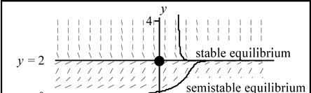
Semistable Equilibrium

19. () 2 1 yy ′ =−

We draw upward arrows on the y-axis for 1 y ≠

to indicate the solution is increasing. When 1 y =

we have a constant solution.

equilibrium

Because the slope lines have positive slope both above and below the constant solution ( ) 1 yt ≡ , we say that the solution ( ) 1 yt ≡ , or the point 1, is semistable (stable from below, unstable from above). In other words, if a solution is perturbed from the value of 1 to a value below 1, the solution will move back towards 1, but if the constant solution ( ) 1 yt ≡ is perturbed to a value larger than 1, it will not move back towards 1. Semistable equilibria are customarily noted with half-filled circles.

Gompertz Equation () 1ln dyyby dt =−

20. (a) Letting ln zy = and using the chain rule we get

Hence, the Gompertz equation becomes dzabz dt = .

(b) Solving this DE for z we find () ztCebta b = +

Substituting back ln zy = gives () abCebtytee =

Using the initial condition ( ) 0 0 yy = , we finally get 0 ln Cya b =

SECTION 2.5 Nonlinear Models: Logistic Equation 165

Fitting the Gompertz Law

21. (a) From Problem 20, () abcebtytee = where 0 ln a cyb =− . In this case ( ) 01 y = , ( ) 22 y = . We note ( ) ( ) 242810yy ≈ ≈ means the limiting value ab e has been reached. Thus 10 ab e = , so

a b =≈ The constant ln102.32.3 a c b =−=−=− . Hence,

Solving for b:

and 2.3 ab = gives 0.4105 a ≈ . (b) The logistic equation

has solution

Gompertz

166 CHAPTER 2 Linearity and Nonlinearity We have 10 L = and 0 1 y = , so

Autonomous Analysis

22. (a) 2 yy ′ =

(b) One semistable equilibrium at ( ) 0 yt ≡ is stable from below, unstable from above.

23. (a) ( ) 1 yyy ′ =−− (b) The equilibrium solutions are ( ) 0 yt ≡ , ( ) 1 yt ≡ . The solution ( ) 0 yt ≡ is stable. The solution ( ) 1 yt ≡ is unstable.

24. (a) 11yy yyLM ⎛⎞⎛⎞ ′ =−−−⎜⎟⎜⎟

2.5 Nonlinear Models: Logistic Equation 167

, ( ) ( ) 110.5 yyyy ′ =−−−

(b) The equilibrium points are 0 y = , L, M. 0 y = is stable. yM = is stable if ML > and unstable if ML < . yL = is stable if ML < and unstable if ML > .

stable equilibrium unstable equilibrium stable equilibrium

25. (a) yyy ′ =−

Note that the DE is only defined for 0 y ≥ .

(b) The constant solution ( ) 0 yt ≡ is stable, the solution ( ) 1 yt ≡ is unstable.

26. (a) () 2 1 yky ′ =− , 0 k >

(b) The constant solution ( ) 1 yt ≡ is semi-stable (unstable above, stable below).

27. (a) ( ) 22 4 yyy ′ =−

(b) The equilibrium solution ( ) 2 yt ≡ is stable, the solution ( ) 2 yt ≡− is unstable and the solution ( ) 0 yt ≡ is semistable.

Stefan’s Law Again

28. ( ) 44TkMT ′ =−

The equation tells us that when 0 TM < < , the solution ( ) TTt = increases because 0 T ′ > , and when MT < the solution decreases because 0 T ′ < . Hence, the equilibrium point ( ) TtM ≡ is stable. We have drawn the directional field of Stefan’s equation for 3 M = , 0.05 k =

0.05344 dT T dt =−

To M > gives solutions falling to M.

To M < gives solutions rising to M

These observations actions match intuition and experiment.

Hubbert Peak

29. (a) From even a hand-sketched logistic curve you can graph its slope y ′ and find a roughly bell-shaped curve for ( ) yt ′ . Depending on the scales used, it may be steeper or flatter than the bell curve shown in Fig. 1.3.5.

SECTION 2.5 Nonlinear Models: Logistic Equation 169

(b) For a pure logistic curve, the inflection point always occurs when 2 L y =

However, if we consider models different from the logistic model that still show similar solutions between 0 and the nonzero equilibrium, it is possible for the inflection point to be closer to 0. When this happens oil recovery reaches the maximum production rate much earlier.

inflection point for solid y curve.

inflection point for dashed y curve

Of course the logistic model is a crude model of oil production. For example it doesn’t take into consideration the fact that when oil prices are high, many oil wells are placed into production.

If the inflection point is lower than halfway on an approximately logistic curve, the peak on the y ′ curve occurs sooner and lower creating an asymmetric curve for y ′

(c) These differences may or may not be significant to people studying oil production; it depends on what they are looking for. The long-term behavior, however, is the same; the peak just occurs sooner. After the peak occurs, if the model holds, it is downhill insofar as oil production is concerned. Typical skew of peak position is presented on the figures above.

Useful Transformation

30. ( ) 1 ykyy ′ =−

Letting 1 y z y = yields

Substituting for dy dt from the original DE yields a new equation

which gives the result

170 CHAPTER 2 Linearity and Nonlinearity

Solving this first-order equation for ( ) zzt = , yields ( ) kt ztce = and substituting this in the transformation 1 y z y = , we get 1 ykt ce y = .

Finally, solving this for y gives () 1 1 11 , 11ktkt c yt ece == ++ where 1 0 1 1 c y =−

Chemical Reactions

31. ( ) ( ) 10050 xkxx =−−

The solutions for the given initial conditions are shown on the graph. Note that all behaviors are at equilibrium or flown off scale before 0.1 t = !

The solution curve for ()0150 x = is almost vertical.

(a) A solution starting at ( ) 00 x = increases and approaches 50.

(b) A solution starting at ( ) 075 x = decreases and approaches 50.

stable equilibrium unstable equilibrium

Direction field and equilbrium

Solutions for three given initial conditions.

Noting the location of equilibrium and the direction field as shown in a second graph leads to the following conclusions: Any (0)100 x > causes ( ) xt to increase without bound and fly off scale very quickly. On the other hand, for any ( ) ( ) 00,100 x ∈ the solution will approach an equilibrium value of 50, which implies the tiniest amount is sufficient to start the reaction.

If you are looking for a different scenario, you might consider some other modeling options that appear in Problem 32.

SECTION 2.5 Nonlinear Models: Logistic Equation 171

General Chemical Reaction of Two Substances ()(), dxmnkaxbxab dt = −−<

32. (a), (b) We consider the four cases when the exponents are even positive integers and/or odd positive integers. In each case, we analyze the sign of the derivative for different values of x. For convenience we pick 1 a = , 2 b = , k = 1.

• ()() 12eveneven dx xx dt =−− .

We have drawn a graph of dx dt versus x.

By drawing arrows to the right when dx dt is positive and arrows to the left when dx dt is negative, 2 x 1 3 semistablesemistable

Both even exponents

we have a horizontal phase line for ( ) xt . We also see that both equilibrium solutions ( ) 1 xt ≡ , ( ) 2 xt ≡ are unstable; although both are semistable; stable from below and unstable from above.

• ()() 12evenodd dx xx dt =−−

Here ( ) 1 xt ≡ is unstablealthough it is stable from below. The solution ( ) 2 xt ≡ is stable. 2 x 1 –1 1 3 semistable stable

Even and odd exponents

dxdt

172 CHAPTER 2 Linearity and Nonlinearity

• ()() 12oddeven dx xx dt =−− .

Here ( ) 2 xt ≡ is semistable,stable from above and unstable from below. The solution ( ) 1 xt ≡ is stable.

2 x 1 –1 1 3 stable semistable dxdt

Odd and even exponents

• ()() 12oddodd dx xx dt =−− .

Here the smaller of the two solutions, ( ) 1 xt ≡ , is stable; the larger solution, ( ) 2 xt ≡ , is unstable.

Solving the Threshold Equation

33. 1 y yryT ⎛⎞ ′ =−−⎜⎟

Introducing backwards time t τ =− , yields

Hence, if we run the threshold equation

backwards, we get

Equivalently it also yields the first-order equation

2 x 1 –1 1 3 stableunstable dxdt

Both odd exponents

SECTION 2.5 Nonlinear Models: Logistic Equation 173 which is the logistic equation with LT = and t τ = . We know the solution of this logistic equation to be

() 0 11Tr y T y e τ τ = +−

We can now find the solution of the threshold equation by replacing τ by t , yielding

() 0 11Trt y T yt e = +−

Limiting Values for the Threshold Equation

34. 1 y yryT ⎛⎞ ′ =−−⎜⎟ ⎝⎠

(a) For 0 0 yT<< as t →∞ the denominator of

0 11Trt y T yt e = +− goes to plus infinity and so ( ) yt goes to zero.

(b) For 0 yT > the denominator of

0 11Trt y T yt e = +− will reach zero (causing the solution to “blow up”) when 0 110 Trt e y ⎛⎞ + ⎜⎟−= ⎝⎠

Solving for t gives the location of a vertical asymptote on the ty graph * 0 0 1 ln ty ryT ⎛⎞ = ⎜⎟ ⎝⎠ .

CHAPTER 2 Linearity and Nonlinearity

Pitchfork Bifurcation

35. ( ) 32 yyyyy αα ′ =−=−

(a) For 0 α ≤ the only real root of ( ) 2 0 yy α = is 0 y = . Because ( ) 2 0 yyy α ′ = −< for 0 y > and ( ) 2 0 yyy α ′ =

for 0

< , the equilibrium solution 0 y = is stable.

(b) When 0 α > the equation ( ) 2 0 yyy α ′ =−= has roots 0 y = , α ±

The points y α =± are stable, but 0 y = is unstable as illustrated by graphing a phase line or direction field of () 2 1 yyy ′ =−− .

Another Bifurcation

36. 2 1 yyby ′ =++

Pitchfork bifurcation at ( ) 0, 0

(a) We find the equilibrium points of the equation by setting 0 y ′ = and solving for y. Doing this we get

We see that for 22 b −<< there are no (real) solutions, and thus no equilibrium solutions. For 2 b =− we have the equilibrium solution +1, and for 2 b = + we have equilibrium solution –1. For each 2 b ≥ we have two equilibrium solutions.

(b) The bifurcation points are at 2 b = and 2 b = + . As b passes through –2 (increasing), the number of equilibrium solutions changes from 2 to 1 to 0, and when b passes through +2, the number of equilibrium solutions changes from 0 to 1 to 2.

SECTION 2.5 Nonlinear Models: Logistic Equation 175

(d) For 2 b = and 2 b =− the single equilibrium is semistable. (Solutions above are repelled; those below are attracted.) For 2 b > there are two equilibria; the larger one is unstable and the smaller one is stable. For 2 b < there are no equilibria.

176 CHAPTER 2 Linearity and Nonlinearity

(e) The bifurcation diagram shows the location of equilibrium points for y versus the parameter value b. Solid circles represent stable equilibria; open circles represent unstable equilibria.

Computer Lab: Bifurcation 37. 2 1 ykyy ′ =++

(a) Setting 0 y ′ = yields two equilibria,

Equilibria of 2 1 yyby ′ = ++ versus b

for 1 4 k < ; none for 1 4 k > ; one for 1 4 k = .

(b) The following phase-plane graphs illustrate the bifurcation.

38. 2 yyyk ′ =++

(a) Setting 0 y ′ = yields two equilibria,

2.5 Nonlinear Models: Logistic Equation

(b) The following phase-plane graphs illustrate the bifurcation.

178 CHAPTER 2 Linearity and Nonlinearity

Computer Lab: Growth Equations

39. 1 y yryL ⎛⎞ ′ =−⎜⎟

We graph the direction field of this equation for 1 L = , 0.5 r = , 1, 2, and 5. We keep L fixed because all it does is raise or lower the steady-state solution to yL = . We see that the larger the parameter r, the faster the solution approaches the steady-state L.

continuedonnextpage

SECTION 2.5 Nonlinear Models: Logistic Equation 179

40. 1 y yry T ⎛⎞ ′ =−−⎜⎟ ⎝⎠

See text Figure 2.5.9.

The parameter r governs the steepness of the solution curves; the higher r the more steeply y leaves the threshold level T.

41. ln 1 y yry L ⎛⎞ ′ =−⎜⎟ ⎝⎠

Equilibrium at L ye = ; higher r values give steeper slopes.

42. t yrey β ′ = For larger β or for larger r, solution curves fall more steeply. Unstable equilibrium 1 r = , 1 β =

Suggested Journal Entry

43. Student Project

2.6 Systems of DEs: A First Look

Predicting System Behavior

1. (a) 3 xy yxy ′ = ′ =−

This (linear) system has one equilibrium point at the origin, ( ) ( ) ,0,0xy = , as do all linear systems. The υ- and h-nullclines are respectively, as shown in part (b).

(b)

(d) The equilibrium point (0, 0) is unstable. All solutions tend quickly to 3 x y = then move gradually towards +∞ or ∞ asymptotically along that line. Whether the motion is left or right depends on the initial conditions.

SECTION 2.6 Systems of DEs: A First Look 181

From the intersection of the two nullclines we find two equilibrium points shown in the following figures. We can locate them graphically far more easily than algebraically!

(d) The lower equilibrium point at

is unstable and the upper equilibrium at

11 42(15),(51)

is stable.

Most trajectories spiral counterclockwise toward the first quadrant equilibrium point. However, if the initial condition is somewhat left or below the 4th quadrant equilibrium, they shoot down towards ∞ . We suspect a dividing line between these behaviors, and we will find it in Chapter 6.

From the intersection of the two nullclines we find two equilibrium points (0, 1), (1, 0).

182 CHAPTER 2 Linearity and Nonlinearity

(d) The equilibrium at (1, 0) is unstable; the equilibrium at (0, 1) is stable. Most trajectories seem to be attracted to the stable equilibrium, but those that approach the lower unstable equilibrium from below or form the right will turn down toward the lower right.

4. 22 xxy yxy

(a) This (singular) system has an entire line of equilibrium points on the line 0 xy+= .

(b) The direction field and the line of unstable equilibrium points are shown at the right.

(d) From part (c) we see the equilibrium points on the line 0 xy + = are all unstable. All nonequilibrium trajectories shoot away from the equilibria along straight lines (of slope 2), towards +∞ if the IC is above the line 0 xy + = and toward −∞ if the IC is below 0 xy+= 5. (a) 22 4 3 xxy yxy

Setting 0 x ′ = and 0 y ′ = gives the intersection of the nullclines:

We find no equilibria because the nullclines do not intersect.

SECTION 2.6 Systems of DEs: A First Look 183

(d) There are no equilibria—all solutions head down to lower right.

6. (a) 53 xy yxy ′ = ′ =+

This (linear) system has one equilibrium point at ( ) ( ) ,0,0xy = as do all linear systems. The 64-dollar question is: Is it stable? The υ- and h-nullclines: 0 y = , 530 xy + = , are shown following and indicate that the origin (0, 0) is unstable. Hence, points starting near the origin will leave the origin. We will see later other ways for showing that (0, 0) is unstable.

184 CHAPTER 2 Linearity and Nonlinearity

(c) The direction field and a few solutions are drawn. Note how the solutions cross the vertical and horizontal nullclines

(d) We see from the preceding figure that solutions come from infinity along a line (that is, not a nulllcline), and then if they are not exactly on the line head off either upwards and to the left or downwards and go to the left on another line. Whether they go up or down depends on whether they initially start above or below the line. It appears that points that start exactly on the line will go to (0, 0). We will see later in Chapter 6 when we study linear systems using eigenvalues and eigenvectors that the solutions come from infinity on one eigenvector and go to infinity on another eigenvector.

7. (a) 1 xxy yxy ′ =−− ′ =−

Setting 0 xy ′′ == and finding the intersection of the nullclines: -nullcline -nullcline1 hyx

we find one equilibrium point 11 , 22

. The arrows indicate that it is a stable equilibrium.

(d) The equilibrium is stable; all other solutions spiral into it.

SECTION 2.6 Systems of DEs: A First Look 185

8. (a) 2 xxy yx ′ =+ ′ =

This (linear) system has one equilibrium point at the origin (0, 0), as do all linear systems. The υ- and h-nullclines: 20xy + = , 0 x = , are shown in part (b) and indicate that the origin (0, 0) is unstable. We will see later other ways to show that the system is unstable.

(d) The equilibrium point (0, 0) is unstable. Other solutions come from upper left or the lower right, heading toward origin but veers off towards ±∞ in the upper right or lower left.

Creating a Predator-Prey Model

9. (a) dR dt = 0.15R 0.00015RF

dt = 0.25F + 0.00003125RF

The rabbits reproduce at a natural rate of 15%; their population is diminished by meetings with foxes. The fox population is diminishing at a rate of 25%; this decline is mitigated only slightly by meeting rabbits as prey. Comparing the predator-prey rates in the two populations shows a much larger effect on the rabbit population, which is consistent with the fact that each fox needs several rabbits to survive.

(b) dR dt = 0.15R 0.00015RF 0.1R = 0.05R 0.00015RF

dF dt = 0.25F + 0.00003125RF 0.1F = 0.35F + 0.00003125RF

Both populations are diminished by the harvesting. The equilibrium populations move from (8000, 1000) in Part (a) to (11200, 333) in Part (b), i.e., more rabbits and fewer foxes if both populations are harvested at the same rate. Figures on the next page.

186 CHAPTER 2 Linearity and Nonlinearity

In figures, x and y are measured in thousands. Note that the vertical axes have different scales from the horizontal axes.

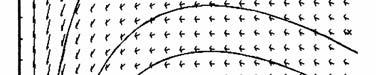
9(a) Equilbrium at (8, 1)

Sharks and Sardines with Fishing

10. (a) With fishing the equilibrium point of the system

9(b) Equilbrium at (11.2, 0.3)

With fishing we increase the equilibrium of the prey ex by f d and decrease the equilibrium of the predator ey by f b

Using the parameters from Example 3 we set 2 a = , 1 b = , 3 c = , 0.5 d = ; the new equilibrium point of the fished model is

SECTION 2.6 Systems of DEs: A First Look 187

4 y 15 0 x

Shark (y) and sardine (x) trajectories

The trajectories are closed curves representing periodic motion of both sharks and sardines. The trajectories look like the trajectories of the unfished case in Example 3 except the equilibrium point has moved to the right (more prey) and down (fewer predators).

(b) With the parameters in part (a) and 0.5 f = the equilibrium point is (7, 1.5). This compares with the equilibrium point (6, 2) in the unfished case.

As the fishing rate f increases from 0 to 2, the equilibrium point moves along the line from the unfished equilibrium at (6, 2) to (10, 0). Hence, the fishing of each population at the same rate benefits the sardines (x) and drives the sharks (y) to extinction. This is illustrated in the figure. 8 4 y x 12 6 2 10 2 (6, 2) (10, 0)

(c) You should fish for sardines when the sardine population is increasing and sharks when the shark population is increasing. In both cases, more fishing tends to move the populations closer to equilibrium while maintaining higher populations in the low parts of the cycle.

(d) If we look at the insecticide model and assume both the good guys (predators) and bad guys (prey) are harvested at the same rate, the good guys will also be diminished and the bad guys peak again. As 1 f → (try 0.8 f = ) the predators get decimated first, then the prey can peak again. If you look at part (a), you see that the predator/prey model does not allow either population to go below zero, as the x- and y-axes are solutions and the solutions move along the axes, thus it is impossible for other solutions to cross either of these axes. You might continue this exploration with the IDE tool, Lotka-Volterra with Harvest, as in Problem 24.

188 CHAPTER 2 Linearity and Nonlinearity

Analyzing Competition Models

11. (120023) dR RRS dt =−− , (500) dS SRS dt =−−

Rabbits are reproducing at the astonishing rate of 1200 per rabbit per unit time, in the absence of competition. However, crowding of rabbits decreases the population at a rate double the population. Furthermore, competition by sheep for the same resources diminishes the rabbit population by three times the number of sheep!

Sheep on the other hand reproduce at a far slower (but still astonishing) rate of 500 per sheep per unit time. Competition among themselves and with rabbits diminishes merely one to one with the number of rabbits and sheep.

Equilibria occur at 00600300 ,,, and 05000200

The equilibria on the axes that are not the origin are the points toward which the populations head. Which species dies out depends on where they start. See Figure, where x and y are measured in hundreds.

12. (120032) dR RRS dt =−− (500) dS SRS dt =−−

The explanations of the equations are the same as those in Problem 11 except that the rabbit population is affected more by the crowding of its own population, less by the number of sheep.

Equilibria occur at 00400200 ,,, or 05000300

SECTION 2.6 Systems of DEs: A First Look 189

In this system the equilibria on the axes are all unstable, so the populations always head toward a coexistence equilibrium at 200 300 ⎡ ⎤ ⎢ ⎥ ⎣ ⎦ . See Figure, where x and y are measured in hundreds.

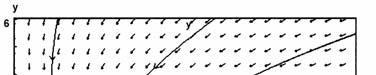
Finding the Model

Example of appropriate models are as follows, with real positive coefficients.

13. 2 xaxbxdxyfx ycydxy ′ =−−− ′ =−+ 14. 2 xaxbxy ycydxyeyz zfzgxhyz ′ = + ′ =−+ ′ =−−

′ =−−−

15. 2 2 xaxbxcxydxz yeyfygxy zhzkxz

′ =−+

Host-Parasite Models

16. (a) A suggested model is

where a, b, c, and d are positive parameters. Here a species of beetle (parasite) depends on a certain species of tree (host) for survival. Note that if the beetle were so effective as to wipe out the entire population of trees, then it would die out itself, which is reflected in our model (note the differential equation in P). On the other hand, in the absence of the beetle, the host tree may or may not die out depending on the size of the parameters a and c. We would probably pick ac > , so the host population would increase in the absence of the parasite. Note too that model says that when the parasite (P) population gets large, it

190 CHAPTER 2 Linearity and Nonlinearity will not destroy the host entirely, as 1 H P + becomes small. The modeler might want to estimate the values of parameters a, b, c, d so the solution fits observed data. The modeler would also like to know the qualitative behavior of ( ) , PH in the PH plane.

Professor Larry Turyn of Wright State University argues for a different model,

′ =− , to better account for the case of very small P.

(b) Many bacteria are parasitic on external and internal body surfaces; some invading inner tissue causing diseases such as typhoid fever, tuberculosis, and pneumonia. It is important to construct models of the dynamics of these complex organisms.

Competition

17. (a) (42) (42) xxxy yyxy ′ =−− ′ =−−

Setting 0 x ′ = and 0 y ′ = we find -nullclines24, 0 -nullclines24, 0. xyx hxyy υ +== +==

Equilibrium points: (0, 0), (0, 2), (2, 0), 44 , 33 ⎛⎞ ⎜⎟ ⎝⎠ . The directions of the solution curves are shown in the figure. 5 0 x y

(b) It can be seen from the figure, that the equilibrium points (0, 0), (0, 2) and (2, 0) are unstable. Only the point 44 , 33 ⎛⎞ ⎜⎟ ⎝⎠ is stable because all solution curves nearby point toward it.

(d) Because all the solution curves eventually reach the stable equilibrium at 44 , 33 ⎛⎞ ⎜⎟ ⎝⎠ , the two species described by this model can coexist.

SECTION 2.6 Systems of DEs: A First Look 191

18. (a) (1) (2) xxxy yyxy ′ =−− ′ =−−

Setting 0 x ′ = and 0 y ′ = we find

+ == + ==

-nullclines1, 0 -nullclines2, 0. xyx hxyy

Equilibrium points: (0, 0), (0, 2), (1, 0).

The directions of the solution curves are shown in the figure.

3 0 x y

(b) It can be seen from the figure, that the equilibrium points (0, 0) and (1, 0) are unstable; the point (0, 2) is stable because all solution curves nearby point toward it.

(d) Because all the solution curves eventually reach the stable equilibrium at (0, 2), the x species always die out and the two species described by this model cannot coexist.

19. (a) (42) (12) xxxy yyxy ′ =−−

=−−

Setting 0 x ′ = and 0 y ′ = we find

+ == + ==

-nullclines24, 0 -nullclines21, 0. xyx hxyy

Equilibrium points: (0, 0), (0, 1), (4, 0).

The directions of the solution curves are shown in the figure. 5 0 x y

(b) It can be seen from the figure, that the equilibrium points (0, 0) and (0, 1) are unstable; the point (4, 0) is stable because all solution curves nearby point toward it.

(d) Because all the solution curves eventually reach the stable equilibrium at (4, 0), the y species always die out and the two species described by this model cannot coexist.

20. (a) (22) (22) xxxy yyxy ′ =−− ′ =−−

Setting 0 x ′ = and 0 y ′ = we find -nullclines22, 0 -nullclines22, 0. xyx hxyy υ +== +==

Equilibrium points: (0, 0), (0, 2), (2, 0), 22 , 33 ⎛⎞ ⎜⎟ ⎝⎠ . The directions of the solution curves are shown in the figure.

3 0 x y

(b) It can be seen from the figure, that the equilibrium points (0, 0) and 22 , 33 ⎛⎞ ⎜⎟ ⎝⎠ are unstable; the points (0, 2) and (2, 0) are stable because all nearby arrows point toward them.

(d) Because all the solution curves eventually reach one of the stable equilibria at (0, 2) or (2, 0), the two species described by this model cannot coexist, unless they are exactly at the unstable equilibrium point 22 , 33 ⎛⎞

⎝⎠ . Which species dies out is determined by the initial conditions.

Simpler Competition

21. ()xxaby ′ =− ()yycdx ′ =−

Setting 0 x ′ = , we find the υ-nullclines are the vertical line 0 x = and the horizontal line a yb =

Setting 0 y ′ = , we find the h-nullclines are the horizontal 0 y = and vertical line c x d = . The

equilibrium points are (0, 0) and , ca db ⎛⎞ ⎜⎟ ⎝⎠ . By observing the signs of x ′ , y ′ we find

0,0xy ′ ′ >> when , ca xydb < < 0,0xy ′ ′ < < when , ca xydb >> 0,0xy ′ ′ < > when , ca xydb >< 0,0xy ′ ′ >< when , ca xydb < >

SECTION 2.6 Systems of DEs: A First Look 193

Hence, both equilibrium points are unstable. We can see from the following direction field (with 1 abcd==== ) that one of two species, depending on the initial conditions, goes to infinity and the other toward extinction. 2 4 y x 4 2

One can get the initial values for these curves directly from the graph.

Nullcline

Patterns

22. (a–e) When the υ-nullcline lies above the h-nullcline, there are three equilibrium points in the first quadrant: (0, 0), 0, d f ⎛⎞

and , 0 a

. The points (0, 0), 0, d f

are unstable and , 0 a b ⎛⎞ ⎜⎟ ⎝⎠ is stable. Hence, only population x survives.

(a)–(b) y

a/c

h -nullcline υ -nullcline

(c)–(d) y x a/c d/f d/ea/b

h-nullcline υ -nullcline

Nullclines and equilibria

Sample trajectories when the υ-nullcline is above the h-nullcline

23. (a–e) When the h-nullcline lies above the υ-nullcline, there are three equilibrium points in the first quadrant: (0, 0), , 0 a b ⎛⎞ ⎜⎟ ⎝⎠ and 0, d f ⎛⎞ ⎜⎟ ⎝⎠ . The points (0, 0), , 0 a b ⎛⎞ ⎜⎟ ⎝⎠ are unstable and 0, d f ⎛⎞ ⎜⎟ ⎝⎠ stable. Hence, only population y survives.

(a)–(b) y a/bd/ex d/f a/c h -nullcline υ -nullcline

Nullclines

(c)–(d) y x d/f a/c a/bd/e h-nullcline υ -nullcline

Sample trajectories when the h-nullcline is above the υ-nullcline

24. (a–e) When the two nullclines intersect as they do in the figure, then there are four equilibrium points in the first quadrant: (0, 0), , 0 a b ⎛⎞ ⎜⎟ ⎝⎠ , 0, d f ⎛⎞ ⎜⎟

, and ( ) , eexy , where ( ) , eexy is the intersection of the lines bxcya + = , exfyd + = . Analyzing the sign of the derivatives in the four regions of the first quadrant, we find that ( ) , eexy is stable and the others unstable. Hence, the two populations can coexist.

(a)–(b) y x d/f a/bd/e a/c h-nullcline υ -nullcline

Nullclines and equilibria

(c)–(d) y x a/c d/f a/bd/e h-nullcline υ -nullcline

Typical trajectories when the nullclines intersect and the slope of the vertical nullcline is more negative.

SECTION 2.6 Systems of DEs: A First Look 195

25. (a–e) When the two nullclines intersect as they do in the figure, then there are four equilibrium points in the first quadrant: (0, 0), , 0 a b ⎛⎞ ⎜⎟ ⎝⎠ , 0, d f ⎛⎞ ⎜⎟ ⎝⎠ , and ( ) , eexy , where ( ) , eexy is the intersection of the lines bxcya + = , exfyd + = . Analyzing the sign of the derivatives in the four regions of the first quadrant, we find , 0 a b ⎛⎞ ⎜⎟ ⎝⎠ and 0, d f ⎛⎞ ⎜⎟ ⎝⎠ are stable and the other two unstable. Hence, only one of the two populations survives, and which survives depends on the initial conditions. See Figures. For initial conditions in the upper region y survives; for initial conditions in the lower region, x survives.

(a)–(b) y x a/c d/ea/b d/f

h -nullcline υ -nullcline

Nullclines and equilibria

Unfair Competition

26. ( ) 1 xaxbxcxy ydyexy ′ =−− ′ =−

h -nullcline

(c)–(d) y x d/f a/c d/ea/b

υ -nullcline

Typical trajectories when the nullclines intersect and the slope of the h-nullcline is more negative.

Setting 0 xy ′′ == , we find three equilibrium points: ( ) 0,0, 1 , 0 b ⎛⎞ ⎜⎟ ⎝⎠ , and , debd a ece ⎛⎞ ⎜⎟ ⎝⎠ .

The point (0, 0) corresponds to both populations becoming extinct, the point 1 , 0 b ⎛⎞ ⎜⎟ ⎝⎠ corresponds to the second population becoming extinct, and the point , debd a ece ⎛⎞ ⎜⎟ ⎝⎠ corresponds to either a stable coexistent point or an unstable point. If we take the special case where 1 d be > , e.g., ( ) 1 0.5 xxxxy yyxy ′ = ′ =−

196 CHAPTER 2 Linearity and Nonlinearity

where 1 abce==== , 0.5 d = , we have the equilibrium points (0, 0), (1, 0), and (0.5, 0.5). If we draw two nullclines; v-nullcline: 1 yx = , h-nullcline: 0.5 x = , as shown following we see that the equilibrium point (0.5, 0.5) is unstable. Hence, the two species cannot coexist.

Nullclines and equilibria for 1 d be >

Sample trajectories for 1 d be >

The reader must check separately the cases where 1 d be = or 1 d be < .

Basins of Attraction

27. Adding shading to the graph obtained in Problem 2 shows the basis of the stable equilibrium at ()

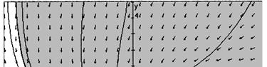
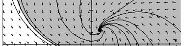
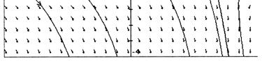
28. Adding shading to the graph obtained in Problem 3 shows the basis of the stable equilibrium at (0, 1).

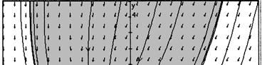
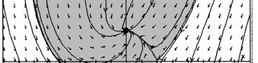
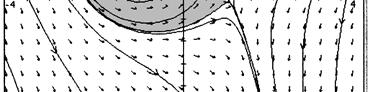
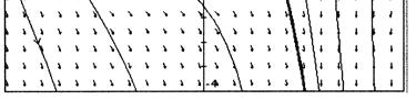
29. Adding shading to the graph obtained in Problem 18 shows that the entire first and second quadrants are the basin of attraction for the stable equilbrium at (0, 2).

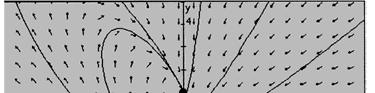
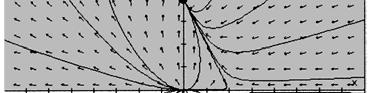
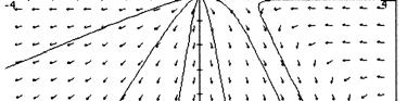
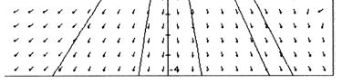
30. The graph obtained in Problem 21 has no stable equilibrium, but we say that there are three basins:

For x > y and y > 0, trajectories are attracted to (0, ∞).

For x > 0 and x < y, trajectories are attracted to (∞, 0).

For x < 0 and y < 0, trajectories are attracted to (−∞, −∞).

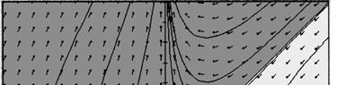
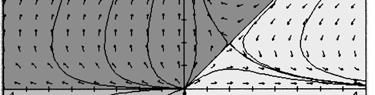
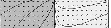
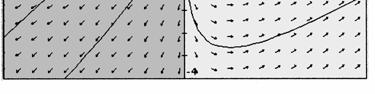
Computer Lab: Parameter Investigation

31. Hold three of the parameters constant and observe how the fourth parameter affects the behavior of the two species. See if the behavior makes sense in your understanding of the model. Keep in mind that parameter Ra is a measure of how well the prey grows in the absence of the predator (large Ra for rabbits), Fa is a measure of how fast the predator population will decline when the prey is absent (large Fa if the given prey is the only source of food for the predator), Rc is a measure of how fast the prey’s population declines per number of prey and predators, and Fc is a measure of how fast the predator’s population increases per number of prey and predators. Even if you are not a biology major, you may still ponder the relative sizes of the four parameters in the two predator–prey systems: foxes and rabbits, and ladybugs and aphids. You can use these explanations to reach the same conclusions as in Problem 9.

Computer Lab: Competition Outcomes

32. (a) Using the IDE software, hold all parameters fixed except one and observe how the last parameters affects the solution. See if the behavior of the two species makes sense in your understanding of the model. Play a mind game and predict if there will be coexistence between the species, whether one becomes extinct, and so on, before you make the parameter change.

Note that in the IDE tool, Competitive Exclusion, there are six parameters; 1K , 1B , 1r , 2 K , 2B , and 2r . The parameters in our text called Ra , Rb , Rc , Fa , Fb , and Fc and enter the equations slightly differently. The reason for this discrepancy is due to the way the parameters in the IDE software affect the two isoclines, called the 1N and 2 N isoclines in the IDE software.

By changing the parameters 1K and 2 K in the IDE software, you simply move the respective isoclines in a parallel direction. The parameters 1B , 2B change the slopes of the nullclines. And finally, the parameters 12 , rr do not affect the nullclines, but affect the direction field or the transient part of the solution.

Your hand-sketched phase plane for the four cases should qualitatively look like the following four pictures, with the basins of attraction colored for each equilibrium.

Case 1: Population x dies out

SECTION 2.6 Systems of DEs: A First Look 199

Case 2: Population y dies out () () 42 12 xxxy

Case 3: Populations coexist

Case 4: One of the populations dies out () () 22 22 xxxy

Of the four different scenarios to the competitive model, in only one (Case 3) can both species coexist. In the other three cases one of the two dies out. In Case 4 the species that dies out depends on the initial conditions, and in Case 1 and 2 one species will die out regardless of the initial condition. Note too that in all four cases if one population initially starts at zero, it remains at zero.

200 CHAPTER 2 Linearity and Nonlinearity

(b) The basins of attraction for each stable equilibrium are shown for each of the four cases. Compare with the figures in part (a).

Suggested Journal Entry

33. Student Project

CASProject2A HeatingandCooling:TransientandSteady-StateSolutions

InthisprojectyouwilluseyourCAStostudysolutioncurveswhenNewton’sLawofCoolingisusedto modeltemperaturechangesinsideahouse.Ausefulsolutionformulaisderivedandthenusedtoillustrate thenotionsoftransientandsteady-statetemperatureandthetimeconstantassociatedwiththemodel. Using Maple therelevantconceptsandcommandsarefunctiondeﬁnitionsandﬁnetuningofplots.

Userdeﬁnedfunctions

Afunction f isdeﬁnedusingthearrowconstructasin f:=x->x*sin(x) whichdeﬁnes f (x)= x sin x.Onecanalsousethe unapply commandtoconvert,say,anexpression named“Harry”intoafunctionof x named“f ”asin f:=unapply(Harry,x) which constructs f (x)=Harry.

Newton’sLawofCoolingmodelstemperaturechangeusingthediﬀerentialequation y (t)= k[A(t) y(t)]. Here y(t)isthetemperatureinsidethehouseattime t and A(t)istheambienttemperature,i.e.the temperatureoutsidethehouse.Theletter k representsapositiveconstant.Ifthereisaheatsource(orsink) inthehousethatcausesachangeinthetemperatureattherate H(t)themodelis

y (t)= k[A(t) y(t)]+ H(t)

TheSolutionFormula. Thisisalinearequation: y (t)+ ky(t)= kA(t)+ H(t)

Theintegratingfactoris µ = ekt so,aftermultiplyingthemodelequationby ekt ,itsimpliﬁesto

Integratewithrespectto t toobtain

andthegeneralsolutionis

Forourpurposesitwillbeconvenienttomaketheantiderivativeexplicitandwritethegeneralsolutionin theform y(t)= Ce kt + t 0 e k(t τ ) kA(τ )+ H(

) dτ .Thisisespeciallynicebecausesubstitutionof t =0 revealsthat C = y(0).Denoting y(0)as y0 wehavearrivedatasolutionformulathatisasusefulasitis beautiful.

TheTimeConstant. Theﬁrstterminthesolutionformulaistheretosatisfytheinitialcondition.Itis referredtoasa transientterm becauseevery1/k secondsitdecreasesby37%(e 1 =0 368).In5 · 1 k seconds thistermwillbelessthan0 7%ofitsinitialvalue,eventuallydisappearingaltogether.Thenumber1/k is calledthe timeconstant.Inanyplotthetransientsinthesolutionwilldisappearinabout5 · 1 k seconds.

Example. It’sacoldwinterevening.Atmidnightthehousetemperatureis25◦ F.Assumethattheoutside temperaturevariesdailyfromalowof15◦ atmidnighttoahighof35◦ at12noon.Thefurnaceissetto cycleonandoﬀperiodicallyprovidingenoughheattomakethetemperatureinsidethehouseincreaseat therateof12◦ anhouratmidnightandattherateof4◦ anhouratnoon.Usethesolutionformuladerived abovetoobtainplotsoftheinsidetemperatureovera72hourperiodbeginningat12midnight(t =0). Assumethat k =0 2.

Theﬁrstentrydeﬁnesthefunctions A(t)and H(t)andplotsthemovera24hourperiod.

>A:=t->25-10*cos(2*Pi*t/24): H:=t->8+4*cos(2*Pi*t/24):

plot([A(t),H(t)],t=0..24,0..40,color=[blue,red],thickness=[2,1], tickmarks=[[4*n$n=0..6],[5*n$n=0..8]]);

Theambienttemperatureistheupper(blue)curve.Thelower(red)curve istherateofchangeoftheinsidetemperatureovera24hourtimeperiod.

Nowdeﬁne y0 and k andevaluatethesolutionformula.The unapply commandmakesthesolutionexpressionintothefunction y.Thesolutionformulaisthendisplayedusing3digitapproximationsforthe constants.Thegraphoftheinsidetemperaturefollows.Wehavealsoincludedthegraphoftheoutside temperatureandthecurveshowingthefurnace’scontributiontorateofchangeof y(t).

>y0:=25:k:=0.2:

>y0*exp(-k*t)+int(exp(-k*(t-tau))*(k*A(tau)+H(tau)),tau=0..t): y:=unapply(%,t):#Thepercentsignreferstothelastoutput. ’y(t)’=evalf[3](y(t));

>plot([y(t),A(t),H(t)],t=0..72,0..80,color=[green,blue,red], thickness=[2,2,1],tickmarks=[[4*n$n=0..18],[10*n$n=0..8]]);

Observethat

Thehighest(green)curveis y(t),thetemperatureinsidethehouseattime t. Themiddle(blue)andlowest(red)curvesareasabove.

Integrationproducedanothertransientinthesolutionformula.Itisalsotheretoaccommodateinitial conditionsandhasthesametimeconstant: 1 0 2 =5hours.Thetransientsvanishinabout25hours. Thetermsthatremainafterthetransientsaregonearereferredtoasthe steady-state termsinthe solution.Inthisexampleweseeasinusoidoscillatingaround65◦ withanamplitudeof √

2 = 6 07.Thustheinsidesteady-statetemperaturevariesfromahighof71◦ athour28(4AM)toalow of59◦ 12hourslater(4PM).

Thingsforyoutodo.

1. Getthecodeworking.Thecyclingofthefurnacewassetuptomakethehousewarmquickly. a) Itisclearfromthesolutioncurvethatoncesteady-stateisattained,thehousewillbetoowarm

atnightandtoocoldduringtheday.Changethefurnacecycletostartat4◦ perhourat midnight(t =0)andcycleto12◦ perhouratnoon.Commentontheeﬀectthishasonthehouse temperature,bothtransientandsteady-state.

b) Experimentwiththetimingofthefurnacecycling(alwaysbetween12and4degreesperhour)to attainasteady-statehousetemperaturethatismaximumcloseto12noonandminimumcloseto 12midnight.Arethemaximumandtheminimumvaluesfor y(t)alwaysthesame?Hint.This processwillrequireatimeshiftintheformulafor H(t).

2. Changetheinitialhousetemperatureto70◦.Whateﬀectdoesthischangehaveonthesteady-state temperature?Whateﬀectdoesithaveonthetimeittakesfor y(t)toreachsteady-state?

3. Returnto y0 =25andtheoriginal H(t).Therearefurnacecyclingparameters(max/min)that yieldaconstantsteady-statehousetemperature.Theycanbefoundexperimentallyorbymaking acarefulanalysisoftheintegralformulaforthesolutionthatisobtainedbysubstituting H(t)= 8+ b0 cos(2πt/24).Findtheseparametersanddisplaythesolutioncurve.

4. Trytoobtainafurnaceschedulethatwillbringthehousetoaconstanttemperatureof68degrees.Do itbyexperimentation(CAS),thenverifybyobtainingthesolutionformulaforthiscyclingschedule (paperandpencil).

5. Exploresolutioncurveswhentheambienttemperaturehasavaryingaveragevalue.Thatis, A(t)= a(t) 10cos(2πt/24)forsomefunction a(t).Forexample,startbyassumingthat a(t)isincreasingat therateof2degreesperday: a(t)=25+ 2 24 t.Whateﬀectdoesthishaveonthebehaviorof y(t)?

CASProject2B GrowthEquationsandBifurcations

InthisprojectyouwilluseyourCAStostudygrowthequationsandtheeﬀectofparametersonthesolutions ofﬁrst-order,non-linearequations.SeeExercises35–42inSection2.5ofthetext.Using Maple therelevant conceptsandcommandsare

DEplot

Theprocedurethatdrawsdirectionﬁeldsandnumericallygeneratedsolutioncurves.See CASProject1A. for..doloops

Simpleloopingconstructscanbemadeeasily.Thedatathatiscreatedina for..doloop canbestoredinatable.Thesyntaxisself-explanatory. dsolve

Thecommandthatﬁndssymbolicsolutionsforadiﬀerentialequationandnumericsolutions foraninitialvalueproblem.SeeCASProject1B.

Example1. ConsidertheGompertzgrowthequation y = r 1 ln y L y.Usedirectionﬁeldsandsolution curvestodeterminethesigniﬁcanceoftheparameters r and L.Obtainasymbolicsolution,ifpossible.

Observethat y(t) > 0forall t.Itcanbeseenbyinspectionthatthereisoneequilibriumsolution, y(t) ≡ eL . Thusthevalueoftheparameter L determinesthepositionoftheequilibrium.Weinvestigatetheeﬀect oftheparameter r byexaminingthedirectionﬁeldsandsolutioncurvescorrespondingto y(0)=0 25and y(0)=5when r =1andwhen r =0 5.Inbothcases, L =ln3,so y(t) ≡ 3istheequilibriumsolution.

Thefirstentriesbelowloadthe DEplot package,definetheDE,thendefine L and r forthefirstplot.The secondplotwascreatedafterchanging r to0.5.Thetwoplotsareplacedsidebysideforeasycomparison. Fromthegraphweseethatthevalueof r determinestherateatwhichthesolutionsapproachtheequilibrium point.

>with(DEtools):

>DE:=diff(y(t),t)=r*(1-ln(y(t))/L)*y(t);

>L:=ln(3):r:=1:

DEplot(DE,y(t),t=0..8,y=0..5,arrows=line, dirgrid=[18,11],color=black,scaling=constrained, [[y(0)=0.25],[y(0)=5]],linecolor=black);

Directionﬁeldandsolution, r =1.Directionﬁeldandsolution, r =0 5.

Symbolicsolutionscanbefound. Maple’ssolutionfortheinitialvalue y(0)=0 25,arbitrary r,and L =ln3 isdisplayedbelow.Checkitbysubstitutingintothediﬀerentialequation.

>unassign(’r’);

dsolve({DE,y(0)=0.25});

y(t)=3e

Example2. Considerthediﬀerentialequation y = ky2 + y +1.Determinethesigniﬁcanceoftheparameter k onthenatureoftheequilibriumpoints.Obtainsymbolicsolutions,ifpossible.

Foraﬁxed k solvetheequation ky2 + y +1=0for y toseethatif k =0,thentheequilibriumpointsare y = 1±√1 4k 2k

If k> 1/4,thentherearenoequilibriumsolutions.Allsolutionsincreasewithoutboundas t →∞

If k =1/4,then y(t) ≡−2istheonlyequilibriumsolution.Moreover,thediﬀerentialequationis y = 1 4 (y +2)2 soallothersolutionsareincreasingandthisisasemistableequilibriumpoint.Solutions approach y = 2frombelowandﬂowawayfromabove.

If1/4 >k> 0,thentherearetwoequilibriumpoints, y1 <y2 < 0.Sincethediﬀerentialequationhas theform y = k(y y1 )(y y2 )with k positive, y1 isastableequilibriumand y2 isunstable.

If k =0,thereisoneequilibrium, y0 = 1.Sincethediﬀerentialequationis y = y +1,thisequilibrium isunstable.

If0 >k> −∞,thentherearetwoequilibriumpointsoncemore, y1 < 0 <y2 .Thediﬀerential equationhastheform y = k(y y1 )(y y2 )with k negative,so y1 isanunstableequilibriumand y2 isstable.

Theplotbelow,calleda bifurcationdiagram,showswherethesepointsareforeach k value.Notethatthe curveissimplytheimplicitplotoftheequation ky2 + y +1=0inthe(k,y)-plane.Tointerpretthisplot, sketchaverticallineatany k-value.Wherethatlineintersectsthecurvesyouwillﬁndthe y-valuesthatare theequilibriafortheDEwiththat k-value.

>with(plots):

>display(implicitplot(k*y^2+y+1=0,k=-3..1,y=-4..4,color=black), plot([[0,t,t=-4..4],[t,0,t=-4..1],[[0.25,-2]],[[0,-1]]], style=[line,line,point,point],symbolsize=18,color=black), view=[-3..1,-4..4],tickmarks=[4,4],axes=boxed, labels=["PARAMETERVALUE,k","EQUILIBRIA,y"], labeldirections=[horizontal,vertical]);

Thebifurcationdiagramfor y = ky2 + y +1. Sincethenumberandthenatureoftheequilibriumpointschangesatthevalues k =0and k =1/4,these arethebifurcationpoints.Seethecorrespondingpointsinthediagram.Thefollowingtablesummarizes thisinformation.

IntervalNumberofEquilibriaNature

∞ >k> 1 4 none

k = 1 4 one semistable

1 4 >k> 0two stable<unstable k =0one unstable

0 >k> −∞ two unstable<stable

Maple’s dsolve procedurecomesupwiththefollowingsymbolicsolutiontothisequation.

>dsolve(diff(y(t),t)=k*y(t)^2+y(t)+1);

Thingsforyoutodo.

1. UsedirectionﬁeldsandsolutioncurvessimilartotheonesshowninExample1todeterminethe signiﬁcanceoftheparametersinthethresholdequationandtheequationfordecayingexponentialrate inExercises40and42ofSection2.5.Obtainsymbolicsolutionsifyoucan.

2. Makeabifurcationanalysisfortheparameter k intheequation y = y2 + y + k (Exercise38inSection 2.5).Includethecalculationoftheequilibriumsolutionsforeach k,abifurcationdiagram,anda bifurcationtablesimilartotheonesshowninExample2.Obtainasymbolicsolutionifyoucan.