Solutions for Elementary Statistics Using The Ti 83 84 Plus Calculator 5th Us Edition by Triola
Chapter 2: Exploring Data with Tables and Graphs
Section 2-1: Frequency Distributions for Organizing and Summarizing Data
1. The table summarizes 50 service times. It is not possible to identify the exact values of all of the original times.
2. The classes of 60–120, 120–180, …, 300–360 overlap, so it is not always clear which class we should put a value in. For example, the value of 120 could go in the first class or the second class. The classes should be mutually exclusive.
3.
4. The sum of the relative frequencies is 125%, but it should be 100%, with a small round off error. All of the relative frequencies appear to be roughly the same, but if they are from a normal distribution, they should start low, reach a maximum, and then decrease.
5. Class width: 10
Class midpoints: 24.5, 34.5, 44.5, 54.5, 64.5, 74.5, 84.5
Class boundaries: 19.5, 29.5, 39.5, 49.5, 59.5, 69.5, 79.5, 89.5
Number: 87
6. Class width: 10
Class midpoints: 24.5, 34.5, 44.5, 54.5, 64.5, 74.5
Class boundaries: 19.5, 29.5, 39.5, 49.5, 59.5, 69.5, 79.5
Number: 87
7. Class width: 100
Class midpoints: 49.5, 149.5, 249.5, 349.5, 449.5, 549.5, 649.5
Class boundaries: –0.5, 99.5, 199.5, 299.5, 399.5, 499.5, 599.5, 699.5
Number: 153
8. Class width: 100
Class midpoints: 149.5, 249.5, 349.5, 449.5, 549.5
Class boundaries: 99.5, 199.5, 299.5, 399.5, 499.5, 599.5
Number: 147
9. No. The maximum frequency is in the second class instead of being near the middle, so the frequencies below the maximum do not mirror those above the maximum.
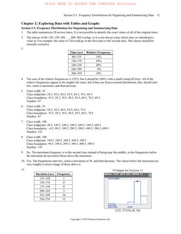
10. Yes. The frequencies start low, reach a maximum of 36, and then decrease. The values below the maximum are very roughly a mirror image of those above it. 11. Duration (sec) Frequency
125–149 1
150–174 0
175–199 0
200–224 3
225–249 34
250–274 12
TI Output for Exercise 11
[125, 275] by [0, 36]
12. The intensities do not appear to have a normal distribution.
15. The distribution does not appear to be a normal distribution.
Output for Exercise 12 [0, 5] by [0, 26]
Output for Exercise 13
14
Output for Exercise 15
[70, 470] by [0, 26]
16. The distribution does appear to be a normal distribution.
Output for Exercise 16
[30, 270] by [0, 16]
17. Because there are disproportionately more 0s and 5s, it appears that the heights were reported instead of measured. Consequently, it is likely that the results are not very accurate.
Output for Exercise 17
[0, 10] by [0, 16]
18. Because there are disproportionately more 0s and 5s, it appears that the weights were reported instead of measured. Consequently, it is likely that the results are not very accurate.
Output for Exercise 18
TI
TI
TI
19. The actresses appear to be younger than the actors.
When Oscar Was Won
20. There do appear to be differences, but overall they are not very substantial differences.
23. No. The highest relative frequency of 24.8% is not much higher than the others.
24. Yes, it appears that births occur on the days of the week with frequencies that are about the same.
25. Yes, the frequency distribution appears to be a normal distribution.
26. Yes, the frequency distribution appears to be a normal distribution.
200] by [0, 135]
Output for Exercise 26
27. Yes, the frequency distribution appears to be a normal distribution.
[40, 115] by [0, 135]
TI Output for Exercise 27
[0, 5] by [0, 190]
TI Output for Exercise 25
[80,
TI
28. No, the frequency distribution does not appear to be a normal distribution.
30.0–39.9 1
40.0–49.9 1 TI Output for Exercise 28
29. An outlier can dramatically increase the number of classes.
[0, 50] by [0, 550]
Section 2-2: Histograms
1. The histogram should be bell-shaped.
2. Not necessarily. Because the sample subjects themselves chose to be included, the voluntary response sample might not be representative of the population.
3. With a data set that is so small, the true nature of the distribution cannot be seen with a histogram.
4. The outlier will result in a single bar that is far away from all of the other bars in the histogram, and the height of that bar will correspond to a frequency of 1.
5. 40
6. Approximate values: Class width: 0.1 gram, lower limit of first class: 5.5 grams, upper limit of first class: 5.6 grams
7. The shape of the graph would not change. The vertical scale would be different, but the relative heights of the bars would be the same.
8. 40 of the quarters are “pre-1964” made with 90% silver and 10% copper, and the other 40 quarters are “post1964” made with a copper-nickel alloy. The histogram depicts weights from two different populations of quarters.
9. Because it is far from being bell-shaped, the histogram does not appear to depict data from a population with a normal distribution.
for Exercise 10
The histogram appears to be skewed to the right (or positively skewed).
The histogram appears to be skewed to the right (or positively skewed).
for Exercise 12
12. Because the histogram isn’t close enough to being bell-shaped, it does not appear to depict data from a population with a normal distribution.
The histogram appears to be skewed to the right (or positively skewed).
for Exercise 14
14. Because the histogram is not close enough to being bell-shaped, it does not appear to depict data from a population with a normal distribution.
15. The digits 0 and 5 appear to occur more often than the other digits, so it appears that the heights were reported and not actually measured. This suggests that the data might not be very useful.
16. The digits 0 and 5 appear to occur more often than the other digits, so it appears that the weights were reported and not actually measured. This suggests that the data might not be very useful.
17. The ages of actresses are lower than the ages of actors.
18. Only part (c) appears to represent data from a normal distribution. Part (a) has a systematic pattern that is not that of a straight line, part (b) has points that are not close to a straight-line pattern, and part (d) is really bad because it shows a systematic pattern and points that are not close to a straight-line pattern.
Section 2-3: Graphs That Enlighten and Graphs That Deceive
1. The data set is too small for a graph to reveal important characteristics of the data. With such a small data set, it would be better to simply list the data or place them in a table.
2. No. If the sample is a bad sample, such as one obtained from voluntary responses, there are no graphs or other techniques that can be used to salvage the data.
3. No. Graphs should be constructed in a way that is fair and objective. The readers should be allowed to make their own judgments, instead of being manipulated by misleading graphs.
4. Center, variation, distribution, outliers, change in the characteristics of data over time. The time-series graph does the best job of giving us insight into the change in the characteristics of data over time.
5. The pulse rate of 36 beats per minute appears to be an outlier.
6. There do not appear to be any outliers.
7. The data are arranged in order from lowest to highest, as 36, 56, 56, and so on.
8. The two values closest to the middle are 72 mm Hg and 74 mm Hg.
9. There is a gradual upward trend that appears to be leveling off in recent years. An upward trend would be helpful to women so that their earnings become equal to those of men.
10. The numbers of home runs rose from 1990 to 2000, but after 2000 there has been a gradual decline.
11. Misconduct includes fraud, duplication, and plagiarism, so it does appear to be a major factor.
12. The overwhelming response was that thank-you notes should be sent to everyone who is met during a job interview. Given what is at stake, that seems like a wise strategy.
15. The distribution appears to be skewed to the left (or negatively skewed).
16. The distribution appears to be skewed to the right (or positively skewed).
17. Because the vertical scale starts with a frequency of 200 instead of 0, the difference between the “no” and “yes” responses is greatly exaggerated. The graph makes it appear that about five times as many respondents said “no,” when the ratio is actually a little less than 2.5 to 1.
18. The fare increased from $1 to $2.50, so it increased by a factor of 2.5. But when the larger bill is drawn so that the width is 2.5 times that of the smaller bill and the height is 2.5 times that of the smaller bill, the larger bill has an area that is 6.25 times that of the smaller bill (instead of being 2.5 times its size, as it should be). The illustration greatly exaggerates the increase in the fare.
19. The two costs are one-dimensional in nature, but the baby bottles are three-dimensional objects. The $4500 cost isn’t even twice the $2600 cost, but the baby bottles make it appear that the larger cost is about five times the smaller cost.
20. The graph is misleading because it depicts one-dimensional data with three-dimensional boxes. See the first and last boxes in the graph. Workers with advanced degrees have annual incomes that are roughly 3 times the incomes of those with no high school diplomas, but the graph exaggerates this difference by making it appear that workers with advanced degrees have incomes that are roughly 27 times the amounts for workers with no high school diploma.
21.
Section 2-4: Scatterplots, Correlation, and Regression
1. The term linear refers to a straight line, and r measures how well a scatterplot of the sample paired data fits a straight-line pattern.
2. No. Finding the presence of a statistical correlation between two variables does not justify any conclusion that one of the variables is a cause of the other.
3. A scatterplot is a graph of paired , x y quantitative data. It helps us by providing a visual image of the data plotted as points, and such an image is helpful in enabling us to see patterns in the data and to recognize that there may be a correlation between the two variables.
4. a. 1 b. 0 c. 0 d. –1
5. There does not appear to be a linear correlation between brain volume and IQ score.
Scatterplot for Exercise 5
6. There does appear to be a linear correlation between chest sizes and weights of bears.
Scatterplot for Exercise 6
6
55] by [0, 500]
TI Output for Exercise 5
[1000, 1400] by [90, 115]
TI Output for Exercise
[25,
7. There does appear to be a linear correlation between weight and highway fuel consumption.
for Exercise 7
Scatterplot for Exercise 8
Output for Exercise 7
[2500, 4500] by [20, 40]
for Exercise 8
[72, 79] by [70, 78]
8. There does not appear to be a linear correlation between heights of fathers and the heights of their first sons.
9. With 5 n pairs of data, the critical values are 0.878. Because 0.127 r is between –0.878 and 0.878, evidence is not sufficient to conclude that there is a linear correlation.
10. With 7 n pairs of data, the critical values are 0.754. Because 0.980 r is in the right tail region beyond 0.754, there are sufficient data to conclude that there is a linear correlation.
11. With 7 n pairs of data, the critical values are 0.754. Because 0.987 r is in the left tail region below –0.754, there are sufficient data to conclude that there is a linear correlation.
12. With 10 n pairs of data, the critical values are 0.632. Because 0.017 r is between –0.632 and 0.632, evidence is not sufficient to conclude that there is a linear correlation.
13. Because the -value P is not small (such as 0.05 or less), there is a high chance (83.9% chance) of getting the sample results when there is no correlation, so evidence is not sufficient to conclude that there is a linear correlation.
14. Because the -value P is small (such as 0.05 or less), there is a small chance of getting the sample results when there is no correlation, so there is sufficient evidence to conclude that there is a linear correlation.
15. Because the -value P is small (such as 0.05 or less), there is a small chance of getting the sample results when there is no correlation, so there is sufficient evidence to conclude that there is a linear correlation.
16. Because the -value P is not small (such as 0.05 or less), there is a high chance (96.3% chance) of getting the sample results when there is no correlation, so the evidence is not sufficient to conclude that there is a linear correlation.
Chapter Quick Quiz
1. Class width: 3. It is not possible to identify the original data values.
2. Class boundaries: 17.5 and 20.5; Class limits: 18 and 20.
3. 40
4. 19 and 19
5. Pareto chart
6. histogram
7. scatterplot
8. No, the term “normal distribution” has a different meaning than the term “normal” that is used in ordinary speech. A normal distribution has a bell shape, but the randomly selected lottery digits will have a uniform or flat shape.
9. variation
10. The bars of the histogram start relatively low, increase to some maximum, and then decrease. Also, the histogram is symmetric, with the left half being roughly a mirror image of the right half.
Review Exercises
1.
2. Yes, the data appear to be from a population with a normal distribution because the bars start low and reach a maximum, then decrease, and the left half of the histogram is approximately a mirror image of the right half.
3. By using fewer classes, the histogram does a better job of illustrating the distribution.
TI Output for Exercise 1
[97.0, 99.5] by [0, 8]
4. There are no outliers.
5. No. There is no pattern suggesting that there is a relationship.
6. a. time-series graph
b. scatterplot
c. Pareto chart
7. A pie chart wastes ink on components that are not data; pie charts lack an appropriate scale; pie charts don’t show relative sizes of different components as well as some other graphs, such as a Pareto chart.
8. The Pareto chart does a better job. It draws attention to the most annoying words or phrases and shows the relative sizes of the different categories.
Cumulative Review Exercises 1.
TI Output for Exercise 1
[235, 265] by [0, 10]
2. a. 235 hours and 239 hours
b. 234.5 hours and 239.5 hours
c. 237 hours
3. The distribution is closer to being a normal distribution than the others.
4. Start the vertical scale at a frequency of 2 instead of the frequency of 0.
5. Looking at the stemplot sideways, we can see that the distribution approximates a normal distribution.
6. a. continuous
b. quantitative
c. ratio
d. convenience sample
e. sample
II. How Should Statistics Be Taught?
Elementary Statistics Using the
TI-83/84 Plus Calculator
Fifth Edition
Chapter 2 Exploring
Data with Tables and Graphs
Exploring Data with Tables and Graphs
2-1 Frequency Distributions for Organizing and Summarizing Data
2-2 Histograms
2-3 Graphs that Enlighten and Graphs that Deceive
2-4 Scatterplots, Correlation, and Regression
Key Concept
When working with large data sets, a frequency distribution (or frequency table) is often helpful in organizing and summarizing data. A frequency distribution helps us to understand the nature of the distribution of a data set.
Frequency Distribution
• Frequency Distribution (or Frequency Table)
– Shows how data are partitioned among several categories (or classes) by listing the categories along with the number (frequency) of data values in each of them.
– The smallest numbers that can belong to each of the different classes
• Upper class limits
– The largest numbers that can belong to each of the different classes
• Class boundaries
– The numbers used to separate the classes, but without the gaps created by class limits
Definitions (2 of 2)
• Class midpoints
– The values in the middle of the classes Each class midpoint can be found by adding the lower class limit to the upper class limit and dividing the sum by 2.
• Class width
– The difference between two consecutive lower class limits in a frequency distribution
Procedure for Constructing a Frequency Distribution
(1 of 2)
1. Select the number of classes, usually between 5 and 20.
2. Calculate the class width.
Round this result to get a convenient number. (It’s usually best to round up.)
Procedure for Constructing a Frequency
Distribution (2 of 2)
3. Choose the value for the first lower class limit by using either the minimum value or a convenient value below the minimum.
4. Using the first lower class limit and class width, list the other lower class limits.
5. List the lower class limits in a vertical column and then determine and enter the upper class limits.
6. Take each individual data value and put a tally mark in the appropriate class. Add the tally marks to get the frequency.
Example: McDonald’s Lunch Service Times
(1 of 5)
Using the McDonald’s lunch service times in the first table, follow the procedure shown on the next slide to construct the frequency distribution shown in the second table. Use five classes.
Example: McDonald’s Lunch Service Times (2
of 5)
Step 1: Select 5 as the number of desired classes.
Step 2: Calculate the class width as shown below. Note that we round 45 up to 50,which is a more convenient number.
Example: McDonald’s Lunch Service Times
(3 of 5)
Step 3: The minimum data value is 83, which is not a very convenient starting point, so go to a value below 83 and select the more convenient value of 75 as the first lower class limit.
Step 4: Add the class width of 50 to the starting value of 75 to get the second lower class limit of 125. Continue to add the class width of 50 until we have five lower class limits. The lower class limits are therefore 75, 125, 175, 225, and 275.
Example: McDonald’s Lunch Service Times
(4 of 5)
Step 5: List the lower class limits vertically, as shown below. From this list, we identify the corresponding upper class limits as 124, 174, 224, 274, and 324.
Example: McDonald’s Lunch Service Times (5
of 5)
Step 6: Enter a tally mark for each data value in the appropriate class. Then add the tally marks to find the frequencies shown in the table.
Relative Frequency Distribution (1 of 2)
• Relative Frequency Distribution or Percentage Frequency Distribution
– Each class frequency is replaced by a relative frequency (or proportion) or a percentage.
The frequency for each class is the sum of the frequencies for that class and all previous classes. Cumulative Frequency
Critical Thinking: Using Frequency
Distributions to Understand Data
In statistics we are often interested in determining whether the data have a normal distribution.
1. The frequencies start low, then increase to one or two high frequencies, and then decrease to a low frequency.
2. The distribution is approximately symmetric. Frequencies preceding the maximum frequency should be roughly a mirror image of those that follow the maximum frequency.
Gaps
• The presence of gaps can show that the data are from two or more different populations.
• However, the converse is not true, because data from different populations do not necessarily result in gaps.
2014,
Example: Exploring Data: What Does a Gap Tell Us?
(1 of 2)
The table shown is a frequency distribution of the weights (grams) of randomly selected pennies.
Example: Exploring
Data: What Does a Gap Tell Us? (2 of 2)
• Examination of the frequencies reveals a large gap between the lightest pennies and the heaviest pennies.
• This suggests that we have two different populations: – Pennies made before 1983 are 95% copper and 5% zinc. – Pennies made after 1983 are 2.5% copper and 97.5% zinc.
Combining two or more relative frequency distributions in one table makes comparisons of data much easier.
Example: Comparing McDonald’s
and Dunkin’ Donuts (1 of 2)
The table shows the relative frequency distributions for the drive-through lunch service times (seconds) for McDonald’s and Dunkin’ Donuts.
Example: Comparing McDonald’s and Dunkin’ Donuts (2
of 2)
• Because of the dramatic differences in their menus, we might expect the service times to be very different.
• By comparing the relative frequencies,we see that there are major differences. The Dunkin’ Donuts service times appear to be lower than those at McDonald’s.
2-1 Frequency Distributions for Organizing and Summarizing Data
2-2 Histograms
2-3 Graphs that Enlighten and Graphs that Deceive
2-4 Scatterplots, Correlation, and Regression
Key Concept
While a frequency distribution is a useful tool for summarizing data and investigating the distribution of data, an even better tool is a histogram, which is a graph that is easier to interpret than a table of numbers.
– A graph consisting of bars of equal width drawn adjacent to each other (unless there are gaps in the data)
The horizontal scale represents classes of quantitative data values, and the vertical scale represents frequencies. The heights of the bars correspond to frequency values.
Important Uses of a Histogram
• Visually displays the shape of the distribution of the data
• Shows the location of the center of the data
• Shows the spread of the data
• Identifies outliers
Relative Frequency Histogram
• Relative Frequency Histogram
– It has the same shape and horizontal scale as a histogram, but the vertical scale is marked with relative frequencies instead of actual frequencies.
Critical Thinking Interpreting
Histograms
Explore the data by analyzing the histogram to see what can be learned about “
Data skewed to the right (positively skewed) have a longer right tail.
Skewness (3 of 3)
Data skewed to the left (negative skewed) have a longer left tail.
Assessing Normality with Normal Quantile Plots
(1 of 5)
Criteria for Assessing Normality with a Normal Quantile Plot
• Normal Distribution: The pattern of the points in the normal quantile plot is reasonably close to a straight line, and the points do not show some systematic pattern that is not a straight-line pattern.
Assessing Normality with Normal Quantile Plots
(2 of 5)
Criteria for Assessing Normality with a Normal Quantile Plot
• Not a Normal Distribution: The population distribution is not normal if the normal quantile plot has either or both of these two conditions:
– The points do not lie reasonably close to a straight-line pattern.
– The points show some systematic pattern that is not a straight-line pattern.
Assessing Normality with Normal Quantile Plots
(3 of 5)
Normal Distribution: The points are reasonably close to a straight-line pattern, and there is no other systematic pattern that is not a straight-line pattern.
A graph of quantitative data in which each data value is plotted as a point (or dot) above a horizontal scale of values. Dots representing equal values are stacked.
Graphs that Enlighten: Dotplots (2 of 2)
• Dotplots – Features of a Dotplot
Displays the shape of distribution of data.
It is usually possible to recreate the original list of data values.
Stemplots (1 of 2)
• Stemplots (or stem-and-leaf plot)
– Represents quantitative data by separating each value into two parts: the stem (such as the leftmost digit) and the leaf (such as the rightmost digit).
Stemplots (2 of 2)
• Stemplots (or stem-and-leaf plot)
– Features of a Stemplot
Shows the shape of the distribution of the data.
Retains the original data values.
The sample data are sorted (arranged in order).
Time-Series Graph (1 of 2)
• Time-Series Graph
– A graph of time-series data, which are quantitative data that have been collected at different points in time, such as monthly or yearly
– A graph of bars of equal width to show frequencies of categories of categorical (or qualitative) data. The bars may or may not be separated by small gaps.
Bar Graph
(2 of 2)
Bar Graphs – Feature of a Bar Graph
Shows the relative distribution of categorical data so that it is easier to compare the different categories.
– A Pareto chart is a bar graph for categorical data, with the added stipulation that the bars are arranged in descending order according to frequencies, so the bars decrease in height from left to right.
Pareto Chart (2 of 3)
• Pareto Charts
– Features of a Pareto Chart
Shows the relative distribution of categorical data so that it is easier to compare the different categories.
Draws attention to the more important categories.
Pie Chart (1 of 3) • Pie Charts – A very common graph that depicts categorical data as slices of a circle, in which the size of each slice is proportional to the frequency count for the category
– A graph using line segments connected to points located directly above class midpoint values
– A frequency polygon is very similar to a histogram, but a frequency polygon uses line segments instead of bars.
Frequency Polygon (2 of 3)
• Frequency Polygon
– A variation of the basic frequency polygon is the relative frequency polygon, which uses relative frequencies (proportions or percentages) for the vertical scale.
• Pictographs – Drawings of objects, called pictographs, are often misleading. Data that are one-dimensional in nature (such as budget amounts) are often depicted with two-dimensional objects (such as dollar bills) or threedimensional objects (such as stacks of coins, homes, or barrels).
Graphs That Deceive (4
of 4)
• Pictographs
– By using pictographs, artists can create false impressions that grossly distort differences by using these simple principles of basic geometry:
When you double each side of a square, its area doesn’t merely double; it increases by a factor of four.
When you double each side of a cube, its volume doesn’t merely double; it increases by a factor of eight.
In addition to the graphs we have discussed in this section, there are many other useful graphs -some of which have not yet been created. The world needs more people who can create original graphs that enlighten us about the nature of data.
In The Visual Display of Quantitative Information, Edward Tufte offers these principles:
• For small data sets of 20 values or fewer, use a table instead of a graph.
• A graph of data should make us focus on the true nature of the data, not on other elements, such as eye-catching but distracting design features.
• Do not distort data; construct a graph to reveal the true nature of the data.
• Almost all of the ink in a graph should be used for the data, not for other design elements.
Elementary Statistics Using the
TI-83/84 Plus Calculator
Fifth Edition
Chapter 2 Exploring
Data with Tables and Graphs
Exploring Data with Tables and Graphs
2-1 Frequency Distributions for Organizing and Summarizing Data
2-2 Histograms
2-3 Graphs that Enlighten and Graphs that Deceive
2-4 Scatterplots, Correlation, and Regression
Key Concept
Introduce the analysis of paired sample data.
Discuss correlation and the role of a graph called a scatterplot, and provide an introduction to the use of the linear correlation coefficient.
Provide a very brief discussion of linear regression, which involves the equation and graph of the straight line that best fits the sample paired data.
Scatterplot and Correlation (1 of 2)
• Correlation
– A correlation exists between two variables when the values of one variable are somehow associated with the values of the other variable.
• Linear Correlation
– A linear correlation exists between two variables when there is a correlation and the plotted points of paired data result in a pattern that can be approximated by a straight line.
Scatterplot and Correlation (2 of 2)
• Scatterplot (or Scatter Diagram)
– A scatterplot (or scatter diagram) is a plot of paired (x, y) quantitative data with a horizontal x-axis and a vertical y-axis. The horizontal axis is used for the first variable (x), and the vertical axis is used for the second variable (y).
Example: Waist and Arm
Correlation (1 of 2)
• Correlation: The distinct pattern of the plotted points suggests that there is a correlation between waist circumferences and arm circumferences.
Example: Waist and Arm
Correlation (2 of 2)
• No Correlation: The plotted points do not show a distinct pattern, so it appears that there is no correlation between weights and pulse rates.
The computed value of the linear correlation coefficient, r, is always between −1 and 1.
• If r is close to −1 or close to 1, there appears to be a correlation.
• If r is close to 0, there does not appear to be a linear correlation.
Example: Correlation between Shoe
Print Lengths and Heights? (2 of 2)
It isn’t very clear whether there is a linear correlation.
P-Value – If there really is no linear correlation between two variables, the P-value is the probability of getting paired sample data with a linear correlation coefficient r that is at least as extreme as the one obtained from the paired sample data.
The P-value of 0.294 is high. It shows there is a high chance of getting a linear correlation coefficient of r = 0.591 (or more extreme) by chance when there is no linear correlation between the two variables.
Interpreting a P-Value from the Example Where n = 5
Because the likelihood of getting r = 0.591 or a more extreme value is so high (29.4% chance), we conclude there is not sufficient evidence to conclude there is a linear correlation between shoe print lengths and heights.
Only a small P-value, such as 0.05 or less (or a 5% chance or less), suggests that the sample results are not likely to occur by chance when there is no linear correlation, so a small P-value supports a conclusion that there is a linear correlation between the two variables.
Example: Correlation between Shoe
Print
Lengths
and
Heights
(n = 40)
Example: Correlation between Shoe Print Lengths and Heights
The scatterplot shows a distinct pattern. The value of the linear correlation coefficient is r = 0.813, and the P-value is 0.000. Because the P-value of 0.000 is small, we have sufficient evidence to conclude there is a linear correlation between shoe print lengths and heights.
– Given a collection of paired sample data, the regression line (or line of best fit, or least-squares line) is the straight line that “best” fits the scatterplot of the data.
Example: Regression Line (1 of 2)
Example: Regression Line (2 of 2)
The general form of the regression equation has a y-intercept of b0 = 80.9 and slope b1 = 3.22.