Solutions for Introduction To Graph Theory 2nd Us Edition by West by 6alsm

2.TREES AND DISTANCE

2.1. BASIC PROPERTIES

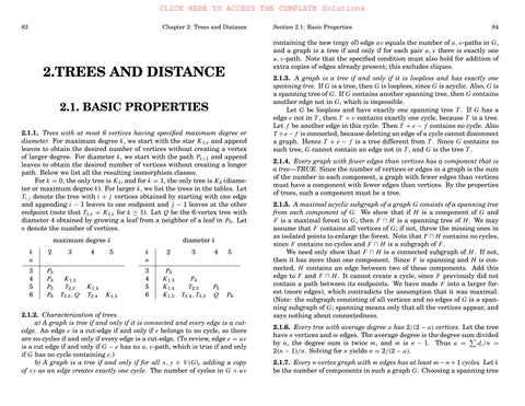
2.1.1. Trees with at most 6 vertices having speciﬁed maximum degree or diameter. For maximum degree k , we start with the star K 1,k and append leaves to obtain the desired number of vertices without creating a vertex of larger degree. For diameter k , we start with the path Pk +1 and append leaves to obtain the desired number of vertices without creating a longer path. Below we list all the resulting isomorphism classes.

For k = 0, the only tree is K 1 , and for k = 1, the only tree is K 2 (diameter or maximum degree k ). For larger k , we list the trees in the tables. Let Ti , j denote the tree with i + j vertices obtained by starting with one edge and appending i 1 leaves to one endpoint and j 1 leaves at the other endpoint (note that T1,k = K 1,k for k ≥ 1). Let Q be the 6-vertex tree with diameter 4 obtained by growing a leaf from a neighbor of a leaf in P5 . Let n denote the number of vertices.

containing the new (copy of) edge u v equals the number of u , v -paths in G , and a graph is a tree if and only if for each pair u , v there is exactly one u , v -path. Note that the speciﬁed condition must also hold for addition of extra copies of edges already present; this excludes cliques.

2.1.3. A graph is a tree if and only if it is loopless and has exactly one spanning tree. If G is a tree, then G is loopless, since G is acyclic. Also, G is a spanning tree of G . If G contains another spanning tree, then G contains another edge not in G , which is impossible.

Let G be loopless and have exactly one spanning tree T . If G has a edge e not in T , then T + e contains exactly one cycle, because T is a tree. Let f be another edge in this cycle. Then T + e f contains no cycle. Also T + e f is connected, because deleting an edge of a cycle cannot disconnect a graph. Hence T + e f is a tree different from T . Since G contains no such tree, G cannot contain an edge not in T , and G is the tree T .

2.1.4. Every graph with fewer edges than vertices has a component that is a tree—TRUE. Since the number of vertices or edges in a graph is the sum of the number in each component, a graph with fewer edges than vertices must have a component with fewer edges than vertices. By the properties of trees, such a component must be a tree.

2.1.2. Characterization of trees.

a) A graph is tree if and only if it is connected and every edge is a cutedge. An edge e is a cut-edge if and only if e belongs to no cycle, so there are no cycles if and only if every edge is a cut-edge. (To review, edge e = u v is a cut edge if and only if G e has no u , v -path, which is true if and only if G has no cycle containing e

b) A graph is a tree if and only if for all x , y ∈ V ( G ), adding a copy of x y as an edge creates exactly one cycle. The number of cycles in G + u v

2.1.5. A maximal acyclic subgraph of a graph G consists of a spanning tree from each component of G . We show that if H is a component of G and F is a maximal forest in G , then F ∩ H is a spanning tree of H . We may assume that F contains all vertices of G ; if not, throw the missing ones in as isolated points to enlarge the forest. Note that F ∩ H contains no cycles, since F contains no cycles and F ∩ H is a subgraph of F . We need only show that F ∩ H is a connected subgraph of H . If not, then it has more than one component. Since F is spanning and H is connected, H contains an edge between two of these components. Add this edge to F and F ∩ H . It cannot create a cycle, since F previously did not contain a path between its endpoints. We have made F into a larger forest (more edges), which contradicts the assumption that it was maximal. (Note: the subgraph consisting of all vertices and no edges of G is a spanning subgraph of G ; spanning means only that all the vertices appear, and says nothing about connectedness.

2.1.6. Every tree with average degree a has 2/(2 a ) vertices. Let the tree have n vertices and m edges. The average degree is the degree sum divided by n , the degree sum is twice m , and m is n 1. Thus a = di / n = 2(n 1)/ n . Solving for n yields n = 2/(2 a ).

2.1.7. Every n -vertex graph with m edges has at least m n + 1 cycles. Let k be the number of components in such a graph G . Choosing a spanning tree

from each component uses n k edges. Each of the remaining m n + k edges completes a cycle with edges in this spanning forest. Each such cycle has one edge not in the forest, so these cycles are distinct. Since k ≥ 1, we have found at least m n + 1 cycles.

2.1.8. Characterization of simple graphs that are forests.

a) A simple graph is a forest if and only if every induced subgraph has a vertex of degree at most 1. If G is a forest and H is an induced subgraph of G , then H is also a forest, since cycles cannot be created by deleting edges. Every component of H is a tree, which is an isolated vertex or has a leaf (a vertex of degree 1). If G is not a forest, then G contains a cycle. A shortest cycle in G has no chord, since that would yield a shorter cycle, and hence a shortest cycle is an induced subgraph. This induced subgraph is 2-regular and has no vertex of degree at most 1.

b) A simple graph is a forest if and only if every connected subgraph is an induced subgraph. If G has a connected subgraph H that is not an induced subgraph, then G has an edge x y not in H with endpoints in V ( H ). Since H contains an x , y -path, H + x y contains a cycle, and G is not a forest. Conversely, if G is not a forest, then G has a cycle C , and every subgraph of G obtained by deleting one edge from C is connected but not induced.

c) The number of components is the number of vertices minus the number of edges. In a forest, each component is a tree and has one less edge than vertex. Hence a forest with n vertices and k components has n k edges.

Conversely, every component with n i vertices has at least n i 1 edges, since it is connected. Hence the number of edges in an n -vertex is n minus the number of components only if every component with n i vertices has n i 1 edges. Hence every component is a tree, and the graph is a forest.

2.1.9. For 2 ≤ k ≤ n 1, the n -vertex graph formed by adding one vertex adjacent to every vertex of Pn 1 has a spanning tree with diameter k . Let v1 , . . . , vn 1 be the vertices of the path in order, and let x be the vertex adjacent to all of them. The spanning tree consisting of the path v 1 , . . . , vk 1 and the edges x vk 1 , . . . , x vn 1 has diameter k .

2.1.10. If u and v are vertices in a connected n -vertex simple graph, and d (u , v ) > 2, then d (u ) + d (v ) ≤ n + 1 d (u , v ). Since d (u , v ) > 2, we have N (u ) ∩ N (v ) = ∅, and hence d (u ) + d (v ) = | N (u ) ∪ N (v )|. Let k = d (u , v ). Between u and v on a shortest u , v -path are vertices x 1 , . . . , x k 1 . Since this is a shortest u , v -path, vertices u , v and x 2 , . . . , x k 2 are forbidden from the neighborhoods of both u and v . Hence | N (u ) ∪ N (v )| ≤ n + 1 k .

The inequality fails when d (u , v ) ≤ 2, because in this case u and v can have many common neighbors. When d (u , v ) = 2, the sum d (u ) + d (v ) can be as high as 2n 4.

2.1.11. If x and y are adjacent vertices in a graph G , then always |d G ( x , z ) d G ( y , z )| ≤ 1. A z , y -path can be extended (or trimmed) to reach x , and hence d ( z , x ) ≤ d ( z , y ) + 1. Similarly, d ( z , y ) ≤ d ( z , x ) + 1. Together, these yield |d ( z , x ) d ( z , y )| ≤ 1.

2.1.12. Diameter and radius of K m ,n . Every vertex has eccentricity 2 in K m ,n if m , n ≥ 2, which yields radius and diameter 2. For K 1,n , the radius is 1 and diameter is 2 if n > 1. The radius and diameter of K 1,1 are 1. The radius and diameter of K 0,n are inﬁnite if n > 1, and both are 0 for K 0,1 .

2.1.13. Every graph with diameter d has an independent set of size at least (1 + d )/2 . Let x , y be vertices with d ( x , y ) = d . Vertices that are nonconsecutive on a shortest x , y -path P are nonadjacent. Taking x and every second vertex along P produces an independent set of size (1 + d )/2 .

2.1.14. Starting a shortest path in the hypercube. The distance between vertices in a hypercube is the number of positions in which their names differ. From u , a shortest u , v -path starts along any edge to a neighbor whose name differ from u in a coordinate where v also differs from u .

2.1.15. The complement of a simple graph with diameter at least 4 has diameter at most 2. The contrapositive of the statement is that if G has diameter at least 3, then G has diameter at most 3. Since G = G , this statement has been proved in the text.

2.1.16. The “square” of a connected graph G has diameter diam ( G )/2 . The square is the simple graph G with x ↔ y in G if and only if d G ( x , y ) ≤ 2. We prove the stronger result that d G ( x , y ) = d G ( x , y )/2 for every x , y ∈ V ( G ). Given an x , y -path P of length k , we can skip the odd vertices along P to obtain an x , y -path of length k /2 in G .

On the other hand, every x , y -path of length l in G arises from a path of length at most 2l in G . Hence the shortest x , y -path in G comes from the shortest x , y -path in G by the method described, and d G ( x , y ) = d G ( x , y )/2 . Hence

diam ( G ) = min x , y d G ( x , y ) = min x ,

2.1.17. If an n -vertex graph G has n 1 edges and no cycles, then it is connected. Let k be the number of components of G . If k > 1, then we adding an edge with endpoints in two components creates no cycles and reduces the number of components by 1. Doing this k 1 times creates a graph with (n 1) + (k 1) edges that is connected and has no cycles. Such a graph is a tree and has n 1 edges. Therefore, k = 1, and the original graph G was connected.

2.1.18. If G is a tree, then G has at least ( G ) leaves. Let k = ( G ). Given n > k ≥ 2, we cannot guarantee more leaves, as shown by growing a path of length n k 1 from a leaf of K 1,k .

Proof 1a (maximal paths). Deleting a vertex x of degree k produces a forest of k subtrees, and x has one neighbor w i in the i th subtree G i . Let Pi be a maximal path starting at x along the edge x w i . The other end of Pi must be a leaf of G and must belong to G i , so these k leaves are distinct.

Proof 1b (leaves in subtrees). Deleting a vertex x of degree k produces a forest of k subtrees. Each subtree is a single vertex, in which case the vertex is a leaf of G , or it has at least two leaves, of which at least one is not a neighbor of x . In either case we obtain a leaf of the original tree in each subtree.

Proof 2 (counting two ways). Count the degree sum by edges and by vertices. By edges, it is 2n 2. Let k be the maximum degree and l the number of leaves. The remaining vertices must have degree at least two each, so the degree sum when counted by vertices is at least k + 2(n l 1) + l . The inequality 2n 2 ≥ k + 2(n l 1) + 1 simpliﬁes to l ≥ k . (Note: Similarly, degree 2(n 1) k remains for the vertices other than a vertex of maximum degree. Since all degrees are 1 or at least 2, there must be at least k vertices of degree 1.)

Proof 3: Induction on the number of vertices. For n ≤ 3, this follows by inspecting the unique tree on n vertices. For n > 3, delete a leaf u . If ( T u ) = ( T ), then by the induction hypothesis T u has at least k leaves. Replacing u adds a leaf while losing at most one leaf from T u . Otherwise ( T u ) = ( T ) 1, which happens only if the neighbor of u is the only vertex of maximum degree in T . Now the induction hypothesis yields at least k 1 leaves in T u . Replacing u adds another, since the vertex of maximum degree in T cannot be a leaf in T u (this is the reason for putting n = 3 in the basis step).

2.1.19. If n i denotes the number of vertices of degree i in a tree T , then i n i depends only on the number of vertices in T . Since each vertex of degree i contributes i to the sum, the sum is the degree-sum, which equals twice the number of edges: 2n ( T ) 2.

2.1.20. Hydrocarbon formulas C k Hl . The global method is the simplest one. With cycles forbidden, there are k + l 1 “bonds” - i.e., edges. Twice this must equal the degree sum. Hence 2(k + l 1) = 4k + l , or l = 2k + 2. Alternatively, (sigh), proof by induction. Basis step (k = 1): The formula holds for the only example. Induction step (k > 1): In the graph of the molecule, each H has degree 1. Deleting these vertices destroys no cycles, so the subgraph induced by the C -vertices is also a tree. Pick a leaf x in this tree. In the molecule it neighbors one C and three H s. Replac-

ing x and these three H s by a single H yields a molecule with one less C that also satisﬁes the conditions. Applying the induction hypothesis yields l = [2(k 1) + 2] 1 + 3 = 2k + 2.

2.1.21. If a simple n -vertex graph G has a decomposition into k spanning trees, and ( G ) = δ ( G ) + 1, then 2k < n , and G has n 2k vertices of degree 2k and 2k vertices of degree 2k 1. Since every spanning tree of G has n 1 edges, we have e ( G ) = k (n 1). Since e ( G ) ≤ n (n 1)/2 edges, this yields k ≤ n /2. Equality requires G = K n , but ( K n ) = δ ( K n ). Thus 2k < n .

To determine the degree sequence, let l be the number of vertices of degree δ ( G ). By the degree-sum formula, n ( G ) l = 2k n 2k . Both sides are between two multiples of n . Since 0 < 2k < n and 0 < l < n , the higher multiple of n is n ( G ) = 2k n , so ( G ) = 2k . It then also follows that l = 2k . Hence there are n 2k vertices of degree 2k and 2k vertices of degree 2k 1.

2.1.22. A tree with degree list k , k 1, . . . , 2, 1, 1, . . . , 1 has 2 + k 2 vertices. Since the tree has n vertices and k 1 non-leaves, it has n k + 1 leaves. Since k i =1 i = k (k + 1)/2, the degrees of the vertices sum to k (k + 1)/2 + n k . The degree-sum is twice the number of edges, and the number of edges is n 1. Thus k (k + 1)/2 + n k = 2n 2. Solving for n yields n = 2 + k 2 .

2.1.23. For a tree T with vertex degrees in {1, k }, the possible values of n ( T ) are the positive integers that are 2 more than a multiple of k 1.

Proof 1 (degree-sum formula). Let m be the number of vertices of degree k . By the degree-sum formula, m k + (n ( T ) m ) = 2n ( T ) 2, since T has n ( T ) 1 edges. The equation simpliﬁes to n ( T ) = m (k 1) + 2. Since m is a nonnegative integer, n ( T ) must be two more than a multiple of k 1. Whenever n = m (k 1) + 2, there is such a tree (not unique for m ≥ 4). Such a tree is constructed by adjoining k 2 leaves to each internal vertex of a path of length m + 1, as illustrated below for m = 4 and k = 5.

Proof 2 (induction on m , the number of vertices of degree k ). We proof that if T has m vertices of degree k , then n ( T ) = m (k 1) + 2 If m = 0, then the tree must have two vertices.

For the induction step, suppose that m > 0. For a tree T with m vertices of degree k and the rest of degree 1, let T be the tree obtained by deleting all the leaves. The tree T is a tree whose vertices all have degree k in T . Let x be a leaf of T . In T , x is adjacent to one non-leaf and to k 1 leaves. Deleting the leaf neighbors of x leaves a tree T with m 1 vertices of degree k and the rest of degree 1. By the induction hypothesis,

n ( T ) = (m 1)(k 1) + 2. Since we deleted k 1 vertices from T to obtain T , we obtain n ( T ) = m (k 1) + 2. This completes the induction step. To prove inductively that all such values arise as the number of vertices in such a tree, we start with K 2 and iteratively expand a leaf into a vertex of degree k to add k 1 vertices.

2.1.24. Every nontrivial tree has at least two maximal independent sets, with equality only for stars. A nontrivial tree has an edge. Each vertex of an edge can be augmented to a maximal independent set, and these must be different, since each contains only one vertex of the edge. A star has exactly two maximal independent sets; the set containing the center cannot be enlarged, and the only maximal independent set not containing the center contains all the other vertices. If a tree is not a star, then it contains a path a , b , c , d . No two of the three independent sets {a , c }, {b , d }, {a , d } can appear in a single independent set, so maximal independent sets containing these three must be distinct.

2.1.25. Among trees with n vertices, the star has the most independent sets (and is the only tree with this many).

Proof 1 (induction on n ). For n = 1, there is only one tree, the star. For n > 1, consider a tree T . Let x be a leaf, and let y be its neighbor. The independent sets in T consist of the independent sets in T x and all sets formed by adding x to an independent set in T x y . By the induction hypothesis, the ﬁrst type is maximized (only) when T x is a star. The second type contributes at most 2 n 2 sets, and this is achieved only when T x y has no edges, which requires that T x is a star with center at y . Thus both contributions are maximized when (and only when) T is a star with center y .

Proof 2 (counting). If an n -vertex tree T is not a star, then it contains a copy H of P4 . Of the 16 vertex subsets of V ( H ), half are independent and half are not. If S is an independent set in T , then S ∩ V ( H ) is also independent. When we group the subsets of V ( T ) by their intersection with V ( T ) V ( H ), we thus ﬁnd that at most half the sets in each group are independent. Summing over all groups, we ﬁnd that at most half of all subsets of V ( T ), or 2n 1 , are independent. However, the star K 1,n 1 has 2n 1 + 1 independent sets.

2.1.26. For n ≥ 3, if G is an n -vertex graph such that every graph obtained by deleting one vertex of G is a tree, then G = C n . Let G i be the graph obtained by deleting vertex vi . Since G i has n 1 vertices and is a tree, e ( G i ) = n 2. Thus n i =1 e ( G i ) = n (n 2). Since each edge has two endpoints, each edge of G appears in n 2 of these graphs and thus is counted n 2 times in the sum. Thus e ( G ) = n . Since G has n vertices and n edges, G must contain a cycle. Since G i

has no cycle, every cycle in G must contain v i . Since this is true for all i , every cycle in G must contain every vertex. Thus G has a spanning cycle, and since G has n edges it has no additional edges, so G = C n .

2.1.27. If n ≥ 2 and d1 , . . . , dn are positive integers, then there exists a tree with these as its vertex degrees if and only if d n = 1 and di = 2(n 1). (Some graphs with such degree lists are not trees.) Necessity: Every nvertex tree is connected and has n 1 edges, so every vertex has degree at least 1 (when n ≥ 2) and the total degree sum is 2(n 1). Sufﬁciency: We give several proofs.

Proof 1 (induction on n ). Basis step (n = 2): The only such list is (1, 1), which is the degree list of the only tree on two vertices. Induction step (n > 2): Consider d1 , . . . , dn satisfying the conditions. Since di > n , some element exceeds 1. Since di < 2n , some element is at most 1. Let d be the list obtain by subtracting 1 from the largest element of d and deleting an element that equals 1. The total is now 2(n 2), and all elements are positive, so by the induction hypothesis there is a tree on n 1 vertices with d as its vertex degrees. Adding a new vertex and an edge from it to the vertex whose degree is the value that was reduced by 1 yields a tree with the desired vertex degrees.

Proof 2 (explicit construction). Let k be the number of 1s in the list d . Since the total degree is 2n 2 and all elements are positive, k ≥ 2. Create a path

For 1 ≤ i ≤ n k , attach di 2 vertices of degree 1 to u i . The resulting graph is a tree (not the only one with this degree list), and it gives the proper degree to u i . We need only check that we have the desired number of leaves. Counting x and y and indexing the list so that d1 , . . . , dn ≥, we compute the number of leaves as

Proof 3 (extremality). Because di = 2(n 1), which is even, there is a graph with n vertices and n 1 edges that realizes d . Among such graphs, let G (having k components) be one with the fewest components. If k = 1, then G is a connected graph with n 1 edges and is the desired tree. If k > 1 and G is a forest, then G has n k edges. Therefore, G has a cycle. Let H be a component of G having a cycle, and let u v be an edge of the cycle. Let H be another component of G . Because each d i is positive, H has an edge, x y . Replace the edges u v and x y by u x and v y (either u v or x y could be a loop.) Because u v was in a cycle, the subgraph induced by V ( H ) is still connected. The deletion of v y might disconnect H , but each piece is now connected to V ( H ), so the new graph G realizes d with fewer components than G , contradicting the choice of G .

2.1.28. The nonnegative integers d 1 ≥ · · · ≥ dn are the degree sequence of some connected graph if and only if di is even, dn ≥ 1, and di ≥ 2n 2. This claim does not hold for simple graphs because the conditions di even, dn ≥ 1, and di ≥ 2n 2 do not prevent d1 ≥ n , which is impossible for a simple graph. Hence we allow loops and multiple edges. Necessity follows because every graph has even degree sum and every connected graph has a spanning tree with n 1 edges. For sufﬁciency, we give several proofs.

Proof 1 (extremality). Since di is even, there is a graph with degrees d1 , . . . , dn . Consider a realization G with the fewest components; since di ≥ 2n 2, G has at least n 1 edges. If G has more than one component, then some component as many edges as vertices and thus has a cycle. A 2-switch involving an edge on this cycle and an edge in another component reduces the number of components without changing the degrees. The choice of G thus implies that G has only one component.

Proof 2 (induction on n ). For n = 1, we use loops. For n = 2, if d 1 = d2 , then we use d1 parallel edges. Otherwise, we have n > 2 or d 1 > d2 . Form a new list d1 , . . . , d n 1 by deleting dn and subtracting dn units from other values. If n ≥ 3 and dn = 1, we subtract 1 from d1 , noting that di ≥ 2n 2 implies d1 > 1. If n ≥ 3 and dn > 1, we make the subtractions from any two of the other numbers. In each case, the resulting sequence has even sum and all entries at least 1.

Letting D = di , we have di = D 2dn . If dn = 1, then D 2dn ≥ 2n 2 2 = 2(n 1) 2. If dn > 1, then D ≥ n dn , and so D 2dn ≥ (n 2)dn ≥ 2n 4 = 2(n 1) 2. Hence the new values satisfy the condition stated for a set of n 1 values. By the induction hypothesis, there is a connected graph G with vertex degrees d1 , . . . , d n 1 .

To obtain the desired graph G , add a vertex v n with di di edges to the vertex with degree di , for 1 ≤ i ≤ n 1. This graph G is connected, because a path from vn to any other vertex v can be construct by starting from v n to a neighbor and continuing with a path to v in G .

Proof 3 (induction on di and prior result). If di = 2n 2, then Exercise 2.1.27 applies. Otherwise, d1 ≥ 2n . If n = 1, then we use loops. If n > 1, then we can delete 2 from d 1 or delete 1 from d1 and d2 without introducing a 0. After applying the induction hypothesis, adding one loop at v1 or one edge from v1 to v2 restores the desired degrees.

2.1.29. Every tree has a leaf in its larger partite set (in both if they have equal size). Let X and Y be the partite sets of a tree T , with | X | ≥ |Y |. If there is no leaf in X , then e ( T ) ≥ 2 | X | = | X | + | X | ≥ | X | + |Y | = n ( T ). This contradicts e ( T ) < n ( T ).

2.1.30. If T is a tree in which the neighbor of every leaf has degree at least 3, then some pair of leaves have a common neighbor.

Proof 1 (extremality). Let P a longest path in T , with endpoint v adjacent to u . Since v is a leaf and u has only one other neighbor on P , u must have a neighbor w off P . If w has a neighbor z = u , then replacing (u , v ) by (u , w , z ) yields a longer path. Hence w is a leaf, and v , w are two leaves with a common neighbor.

Proof 2 (contradiction). Suppose all leaves of T have different neighbors. Deleting all leaves (and their incident edges) reduces the degree of each neighbor by 1. Since the neighbors all had degree at least 3, every vertex now has degree at least 2, which is impossible in an acyclic graph.

Proof 3 (counting argument). Suppose all k leaves of T have different neighbors. The n 2k vertices other than leaves and their neighbors have degree at least 2, so the total degree is at least k + 3k + 2(n 2k ) = 2n , contradicting d (v ) = 2e ( T ) = 2n 2.

Proof 4 (induction on n ( T )). For n = 4, the only such tree is K 1,3 , which satisﬁes the claim. For n > 4, let v be a leaf of T , and let w be its neighbor. If w has no other leaf as neighbor, but has degree at least 3, then T v is a smaller tree satisfying the hypotheses. By the induction hypothesis, T v has a pair of leaves with a common neighbor, and these form such a pair in T .

2.1.31. A simple connected graph G with exactly two non-cut-vertices is a path. Proof 1 (properties of trees). Every connected graph has a spanning tree. Every leaf of a spanning tree is not a cut-vertex, since deleting it leaves a tree on the remaining vertices. Hence every spanning tree of G has only two leaves and is a path. Consider a spanning path with vertices v1 , . . . , vn in order. If G has an edge vi v j with i < j 1, then adding vi v j to the path creates a cycle, and deleting v j 1 v j from the cycle yields another spanning tree with three leaves. Hence G has no edge off the path. Proof 2 (properties of paths and distance). Let x and y be the non-cutvertices, and let P be a shortest x , y -path. If V ( P ) = V ( G ), then let w be a vertex with maximum distance from V ( P ). By the choice of w , every vertex of V ( G ) V ( P ) {w } is as close to V ( P ) as w and hence reaches V ( P ) by a path that does not use w . Hence w is a non-cut-vertex. Thus V ( P ) = V ( G ). Now there is no other edge, because P was a shortest x , y -path.

2.1.32. Characterization of cut-edges and loops.

An edge of a connected graph is a cut-edge if and only if it belongs to every spanning tree. If G has a spanning tree T omitting e , then e belongs to a cycle in T + e and hence is not a cut-edge in G . If e is not a cut-edge in G , then G e is connected and contains a spanning tree T that is also a spanning tree of G ; thus some spanning tree omits e .

An edge of a connected graph is a loop if and only if it belongs to no spanning tree. If e is a loop, then e is a cycle and belongs to no spanning

tree. If e is not a loop, and T is a spanning tree not containing e , then T + e contains exactly one cycle, which contains another edge f . Now T + e f is a spanning tree containing e , since it has no cycle, and since deleting an edge from a cycle of the connected graph T + e cannot disconnect it.

2.1.33. A connected graph with n vertices has exactly one cycle if and only if it has exactly n edges. Let G be a connected graph with n vertices. If G has exactly one cycle, then deleting an edge of the cycle produces a connected graph with no cycle. Such a graph is a tree and therefore has n 1 edges, which means that G has n edges.

For the converse, suppose that G has exactly n edges. Since G is connected, G has a spanning tree, which has n 1 edges. Thus G is obtained by adding one edge to a tree, which creates a graph with exactly one cycle. Alternatively, we can use induction. If G has exactly n edges, then the degree sum is 2n , and the average degree is 2. When n = 1, the graph must be a loop, which is a cycle. When n > 2, if G is 2-regular, then G is a cycle, since G is connected. If G is not 2-regular, then it has a vertex v of degree 1. Let G = G v . The graph G is connected and has n 1 vertices and n 1 edges. By the induction hypothesis, G has exactly one cycle. Since a vertex of degree 1 belongs to no cycle, G also has exactly one cycle.

2.1.34. A simple n -vertex graph G with n > k and e ( G ) > n ( G )(k 1) k 2 contains a copy of each tree with k edges. We use induction on n . For the basis step, let G be a graph with k + 1 vertices. The minimum allowed number of edges is (k + 1)(k 1) k 2 + 1, which simpliﬁes to k 2 . Hence G = K k +1 , and T ⊆ G .

For the induction step, consider n > k + 1. If every vertex has degree at least k , then containment of T follows from Proposition 2.1.8. Otherwise, deleting a vertex of minimum degree (at most k 1) yields a subgraph G on n 1 vertices with more than (n 1)(k 1) k 2 edges. By the induction hypothesis, G contains T , and hence T ⊆ G .

2.1.35. The vertices of a tree T all have odd degree if and only if for all e ∈ E ( T ), both components of T e have odd order. Necessity. If all vertices have odd degree, then deleting e creates two of even degree. By the Degree-sum Formula, each component of T e has an even number of odd-degree vertices. Together with the vertex incident to e , which has even degree in T e , each component of T e has odd order. Sufﬁciency.

Proof 1 (parity). Given that both components of T e have odd order, n ( T ) is even. Now consider v ∈ V ( T ). Deleting an edge incident to v yields a component containing v and a component not containing v , each of odd order. Together, the components not containing v when we delete the various edges incident to v are d (v ) pairwise disjoint subgraphs that together

contain all of V ( T ) {v }. Under the given hypothesis, they all have odd order. Together with v , they produce an even total, n ( T ). Hence the number of these subgraphs is odd, which means that the number of edges in T incident to v is odd.

Proof 2 (contradiction). Suppose that such a tree T0 has a vertex v1 of even degree. Let e1 be the last edge on a path from a leaf to x . Let T1 be the component of T0 e1 containing v1 . By hypothesis, T1 has odd order, and v1 is a vertex of odd degree in T1 . Since the number of odd-degree vertices in T1 must be even, there is a vertex v 2 of T1 (different from v1 ) having even degree (in both T1 and T ).

Repeating the argument, given v i of even degree in Ti 1 , let ei be the last edge on the vi 1 , vi -path in Ti 1 , and let Ti be the component of Ti 1 ei containing vi . Also Ti is the component of T0 ei that contains vi , so Ti has odd order. Since vi has odd degree in Ti , there must be another vertex vi +1 with even degree in Ti .

In this way we generate an inﬁnite sequence v 1 , v2 , . . . of distinct vertices in T0 . This contradicts the ﬁniteness of the vertex set, so the assumption that T0 has a vertex of even degree cannot hold.

2.1.36. Every tree T of even order has exactly one subgraph in which every vertex has odd degree.

Proof 1 (Induction). For n ( T ) = 2, the only such subgraph is T itself. Suppose n ( T ) > 2. Observe that every pendant edge must appear in the subgraph to give the leaves odd degree. Let x be an endpoint of a longest path P , with neighbor u . If u has another leaf neighbor y , add u x and u y to the unique such subgraph found in T { x , y }. Otherwise, d (u ) = 2, since P is a longest path. In this case, add the isolated edge u x to the unique such subgraph found in T {u , x }.

Proof 2 (Explicit construction). Every edge deletion breaks T into two components. Since the total number of vertices is even, the two components of T e both have odd order or both have even order. We claim that the desired subgraph G consists of all edges whose deletion leaves two components of odd order.

First, every vertex has odd degree in this subgraph. Consider deleting the edges incident to a vertex u . Since the total number of vertices in T is even, the number of resulting components other than u itself that have odd order must be odd. Hence u has odd order in G .

Furthermore, G is the only such subgraph. If e is a cut-edge of G , then in G e the two pieces must each have even degree sum. Given that G is a subgraph of T with odd degree at each vertex, parity of the degree sum forces G to e if T e has components of odd order and omit e if T e has components of even order.

Comment: Uniqueness also follows easily from symmetric difference. Given two such subgraphs G 1 , G 2 , the degree of each vertex in the symmetric difference is even, since its degree is odd in each G i . This yields a cycle in G 1 ∪ G 2 ⊆ T , which is impossible.

2.1.37. If T and T are two spanning trees of a connected graph G , and e ∈ E ( T ) E ( T ), then there is an edge e ∈ E ( T ) E ( T ) such that both T e + e and T e + e are spanning trees of G . Deleting e from T leaves a graph having two components; let U , U be their vertex sets. Let the endpoints of e be u ∈ U and u ∈ U . Being a tree, T contains a unique u , u -path. This path must have an edge from U to U ; choose such an edge to be e , and then T e + e is a spanning tree. Since e is the only edge of T between U and U , we have e ∈ E ( T ) E ( T ). Furthermore, since e is on the u , u -path in T , e is on the unique cycle formed by adding e to T , and thus T e + e is a spanning tree. Hence e has all the desired properties.

2.1.38. If T and T are two trees on the same vertex set such that d T (v ) = d T (v ) for each vertex v , then T can be obtained from T using 2-switches (Deﬁnition 1.3.32) with every intermediate graph being a tree. Using induction on the number n of vertices, it sufﬁces to show when n ≥ 4 that we can apply (at most) one 2-switch to T to make a given leaf x be adjacent to its neighbor w in T . We can then delete x from both trees and apply the induction hypothesis. Since the degrees specify the tree when n is at most 3, this argument also shows that at most n 3 2-switches are needed.

Let y be the neighbor of x in T . Note that w is not a leaf in T , since d T (w ) = d T (w ) and x w ∈ E ( T ) and n ≥ 4. Hence we can choose a vertex z in T that is a neighbor of w not on the x , w -path in T . Cutting x y and w z creates three components: x alone, one containing z , and one containing y , w . Adding the edges z y and x w to complete the 2-switch gives x its desired neighbor and reconnects the graph to form a new tree.

2.1.39. If G is a nontrivial tree with 2k vertices of odd degree, then G decomposes into k paths.

Proof 1 (induction and stronger result). We prove the claim for every forest G , using induction on k . Basis step (k = 0): If k = 0, then G has no leaf and hence no edge.

Induction step (k > 0): Suppose that each forest with 2k 2 vertices of odd degree has a decomposition into k 1 paths. Since k > 0, some component of G is a tree with at least two vertices. This component has at least two leaves; let P be a path connecting two leaves. Deleting E ( P ) changes the parity of the vertex degree only for the endpoints of P ; it makes them even. Hence G E ( P ) is a forest with 2k 2 vertices of odd degree. By the induction hypothesis, G E ( P ) is the union of k 1 pairwise edgedisjoint paths; together with P , these paths partition E ( G ).

Proof 2 (extremality). Since there are 2k vertices of odd degree, at least k paths are needed. If two endpoints of paths occur at the same vertex of the tree, then those paths can be combined to reduce the number of paths. Hence a decomposition using the fewest paths has at most one endpoint at each vertex. Under this condition, endpoints occur only at vertices of odd degree. There are 2k of these. Hence there are at most 2k endpoints of paths and at most k paths.

Proof 3 (applying previous result). A nontrivial tree has leaves, so k > 0. By Theorem 1.2.33, G decomposes into k trails. Since G has no cycles, all these trails are paths.

2.1.40. If G is a tree with k leaves, then G is the union of k /2 pairwise intersecting paths. We prove that we can express G in this way using paths that end at leaves. First consider any way of pairing the leaves as ends of k /2 paths (one leaf used twice when k is odd). Suppose that two of the paths are disjoint; let these be a u , v -path P and an x , y -path Q . Let R be the path connecting P and Q in G . Replace P and Q by the u , x -path and the v , y -path in G . These paths contain the same edges as P and Q , plus they cover R twice (and intersect). Hence the total length of the new set of paths is larger than before.

Continue this process; whenever two of the paths are disjoint, make a switch between them that increases the total length of the paths. This process cannot continue forever, since the total length of the paths is bounded by the number of paths ( k /2 ) times the maximum path length (at most n 1). The process terminates only when the set of paths is pairwise intersecting. (We have not proved that some vertex belongs to all the paths.)

Finally, we show that a pairwise intersecting set of paths containing all the leaves must have union G . If any edge e of G is missing, then G e has two components H , H , each of which contains a leaf of G . Since e belongs to none of the paths, the paths using leaves in H do not intersect the paths using leaves in H . This cannot happen, because the paths are pairwise intersecting.

(Comment: We can phrase the proof using extremality. The pairing with maximum total length has the desired properties; otherwise, we make a switch as above to increase the total length.)

2.1.41. For n ≥ 4, a simple n -vertex graph with at least 2n 3 edges must have two cycles of equal length. For such a graph, some component must have size at least twice its order minus 3. Hence we may assume that G is connected. A spanning tree T has n 1 edges and diameter at most n 1. Each remaining edge completes a cycle with edges of T . The lengths of these cycles belong to {3, . . . , n }.

Since there are at least n 2 remaining edges, there are two cycles of the same length unless there are exactly n 2 remaining cycles and they create cycles of distinct lengths with the edge of T . This forces T to be a path. Now, after adding the edge e between the endpoints of T that produces a cycle of length n , the other remaining edges each produce two additional shorter cycles when added. These 2n 6 additional cycles fall into the n 3 lengths {3, . . . , n 1}. Since 2n 6 > n 3 when n ≥ 4, the pigeonhole principle yields two cycles of equal length.

2.1.42. Extendible vertices. In a nontrivial Eulerian graph G , a vertex is extendible if every trail beginning at v extends to an Eulerian circuit. a) v is extendible if and only if G v is a forest.

Necessity. We prove the contrapositive. If G v is not a forest, then G v has a cycle C . In G E (C ), every vertex has even degree, so the component of G E (C ) containing v has an Eulerian circuit. This circuit starts and ends at v and exhausts all edges of G incident to v , so it cannot be extended to reach C and complete an Eulerian circuit of G .

Sufﬁciency. If G v is a forest, then every cycle of G contains v . Given a trail T starting at v , extend it arbitarily at the end until it can be extended no farther. Because every vertex has even degree, the process can end only at v . The resulting closed trail T must use every edge incident to v , else it could extend farther. Since T is closed, every vertex in G E ( T ) has even degree. If G E ( T ) has any edges, then minimum degree at least two in a component of G E ( T ) yields a cycle in G E ( T ); this cycle avoids v , since T exhausted the edges incident to v . Since we have assumed that G v has no cycles, we conclude that G E ( T ) has no edges, so T is an Eulerian circuit that extends T . (Sufﬁciency can also be proved by contrapositive.)

b) If v is extendible, then d (v ) = ( G ). An Eulerian graph decomposes into cycles. If this uses m cycles, then each vertex has degree at most

2m . By part (a) each cycle contains v , and thus d (v ) ≥ 2m . Hence v has maximum degree.

Alternatively, since each cycle contains v , an Eulerian circuit must visit v between any two visits to another vertex u . Hence d (v ) ≥ d (u ).

c) For n ( G ) > 2, all vertices are extendible if and only if G is a cycle. If G is a cycle, then every trail from a vertex extends to become the complete cycle. Conversely, suppose that all vertices are extendible. By part (a), every vertex lies on every cycle. Let C be a cycle in G ; it must contain all vertices. If G has any additional edge e , then following the shorter part of C between the endpoints of e completes a cycle with e that does not contain all the vertices. Hence there cannot be an additional edge and G = C .

d) If G is not a cycle, then G has at most two extendible vertices. From part (c), we may assume that G is Eulerian but not a cycle. If v is extendible, then G v is a forest. This forest cannot be a path, since then G is a cycle or has a vertex of odd degree. Since G v is a forest and not a path, G v has more than ( G v ) leaves unless G v is a tree with exactly one vertex of degree greater than two. If G v has more than ( G v ) leaves, all in N (v ), then no vertex of G v has degree as large as v in G , and by part (b) no other vertex is extendible. In the latter case, the one other vertex of degree d (v ) may also be extendible, but all vertices except those two have degree 2.

2.1.43. Given a vertex u in a connected graph G , there is a spanning tree of G that is the union of shortest paths from u to the other vertices.

Proof 1 (induction on n ( G )). When n ( G ) = 1, the vertex u is the entire tree. For n ( G ) > 1, let v be a vertex at maximum distance from u . Apply the induction hypothesis to G v to obtain a tree T in G v . Shortest paths in G from u to vertices other than v do not use v , since v is farthest from u . Therefore, T consists of shortest paths in G from u to the vertices other than v . A shortest u , v -path in G arrives at v from some vertex of T . Adding the ﬁnal edge of that path to T completes the desired tree in G .

Proof 2 (explicit construction). For each vertex other than u , choose an incident edge that starts a shortest path to u . No cycle is created, since as we follow any path of chosen edges, the distance from u strictly decreases. Also n ( G ) 1 edges are chosen, and an acyclic subgraph with n ( G ) 1 edges is a spanning tree. Since distance from u decreases with each step, the v , u -path in the chosen tree is a shortest v , u -path.

Comment: The claim can also be proved using BFS to grow the tree. Proof 1 is a short inductive proof that the BFS algorithm works. Proof 2 is an explicit description of the edge set produced by Proof 1.

2.1.44. If a simple graph with diameter 2 has a cut-vertex, then its complement has an isolated vertex—TRUE. Let v be a cut-vertex of a simple

graph G with diameter 2. In order to have distance at most 2 to each vertex in the other component(s) of G v , a vertex of G v must be adjacent to v . Hence v has degree n ( G ) 1 in G and is isolated in G .

2.1.45. If a graph G has spanning trees with diameters 2 and l , then G has spanning trees with all diameters between 2 and l .

Proof 1 (local change). The only trees with diameter 2 are stars, so G has a vertex v adjacent to all others. Given a spanning tree T with leaf u , replacing the edge incident to u with u v yields another spanning tree T . For every destroyed path, a path shorter by 1 remains. For every created path, a path shorter by 1 was already present. Hence diam T differs from diam T by at most 1. Continuing this procedure reaches a spanning tree of diameter 2 without skipping any values along the way, so all the desired values are obtained.

Proof 2 (explicit construction). Since G has a tree with diameter 2, it has a vertex v adjacent to all others. Every path in G that does not contain v extends to v and to an additional vertex if it does not already contain all vertices. Hence for k < l there is a path P of length k in G that contains v as an internal vertex. Adding edges from v to all vertices not in P completes a spanning tree of diameter k .

2.1.46. For n ≥ 2, the number of isomorphism classes of n -vertex trees with diameter at most 3 is n /2 . If n ≤ 3, there is only one tree, and its diameter is n 1. If n ≥ 4, every tree has diameter at least 2. There is one having diameter 2, the star. Every tree with diameter 3 has two centers, x , y , and every non-central vertex is adjacent to exactly one of x , y , so d ( x ) + d ( y ) = n . By symmetry, we may assume d ( x ) ≤ d ( y ). The unlabeled tree is now completely speciﬁed by d ( x ), which can take any value from 2 through n /2 . Together with the star, the number of trees is n /2 .

2.1.47. Diameter and radius.

a) The distance function d (u , v ) satisﬁes the triangle inequality: d (u , v ) + d (v , w ) ≥ d (u , w ). A u , v -path of length d (u , v ) and a v , w -path of length d (v , w ) together form a u , w -walk of length l = d (u , v ) + d (v , w ). Every u , w -walk contains a u , w -path among its edges, so there is a u , wpath of length at most l . Hence the shortest u , w -path has length at most l . b) d ≤ 2r , where d is the diameter of G and r is the radius of G . Let u , v be two vertices such that d (u , v ) = d . Let w be a vertex in the center of G ; it has eccentricity r . Thus d (u , w ) ≤ r and d (w , v ) ≤ r . By part (a), d = d (u , v ) ≤ d (u , w ) + d (w , v ) ≤ 2r . c) Given integers r, d with 0 < r ≤ d ≤ 2r , there is a simple graph with radius r and diameter d . Let G = C 2r ∪ H , where H ∼ = Pd r +1 and the cycle shares with H exactly one vertex x that is an endpoint of H . The distance from the other end of H to the vertex z opposite x on the cycle is

d , and this is the maximum distance between vertices. Every vertex of H has distance at least r from z , and every vertex of the cycle has distance r from the vertex opposite it on the cycle. Hence the radius is at least r . The eccentricity of x equals r , so the radius equals r , and x is in the center.

2.1.48. For n ≥ 4, the minimum number of edges in an n -vertex graph with diameter 2 and maximum degree n 2 is 2n 4. The graph K 2,n 2 shows that 2n 4 edges are enough. We show that at least 2n 4 are needed. Let G be an n -vertex graph with diameter 2 and maximum degree n 2. Let x be a vertex of degree n 2, and let y be the vertex not adjacent to x .

Proof 1. Every path from y through x to another vertex has length at least 3, so diameter 2 requires paths from y to all of V ( G ) { x , y } in G x . Hence G x is connected and therefore has at least n 2 edges. With the n 2 edges incident to x , this yields at least 2n 4 edges in G .

Proof 2. Let A = N ( y ). Each vertex of N ( x ) A must have an edge to a vertex of A in order to reach y in two steps. These are distinct and distinct from the edges incident to y , so we have at least | A | + | N ( x ) A | edges in addition to those incident to x . The total is again at least 2n 4. (Comment: The answer remains the same whenever (2n 2)/3 ≤ ( G ) ≤ n 5 but is 2n 5 when n 4 ≤ ( G ) ≤ n 3.)

2.1.49. If G is a simple graph with rad G ≥ 3, then rad G ≤ 2. The radius is the minimum eccentricity. For x ∈ V ( G ), there is a vertex y such that d G ( x , y ) ≥ 3. Let w be the third vertex from x along a shortest x , y -path (possibly w = y ). For v ∈ V ( G ) { x }, if x v / ∈ E ( G ), then x v ∈ E ( G ). Now v w / ∈ E ( G ), since otherwise there is a shorter x , y -path. Thus x , w , v is an x , v -path of length 2 in G . Hence for all v ∈ V ( G ) { x }, there is an x , v -path of length at most 2 in G , and we have ε G ( x ) ≤ 2 and rad ( G ) ≤ 2.

2.1.50. Radius and eccentricity.

a) The eccentricities of adjacent vertices differ by at most 1. Suppose that x ↔ y . For each vertex z , d ( x , z ) and d ( y , z ) differ by at most 1 (Exercise 2.1.11). Hence

ε ( y ) = max z d ( y , z ) ≤ max z (d

+ 1.

Similarly, ε ( x ) ≤ ε ( y ) + 1. The statement can be made more general: |ε ( x ) ε ( y )| ≤ d ( x , y ) for all x , y ∈ V ( G ).

b) In a graph with radius r , the maximum possible distance from a vertex of eccentricity r + 1 to the center of G is r . The distance is at most r , since every vertex is within distance at most r of every vertex in the

center, by the deﬁnitions of center and radius. The graph consisting of a cycle of length 2r plus a pendant edge at all but one vertex of the cycle achieves equality. All vertices of the cycle have eccentricity r + 1 except the vertex opposite the one with no leaf neighbor, which is the unique vertex with eccentricity r . The leaves have eccentricity r + 2, except for the one adjacent to the center.

2.1.51. If x and y are distinct neighbors of a vertex v in a tree G , then 2ε (v ) ≤ ε ( x ) + ε ( y ). Let w be a vertex at distance ε (v ) from v . The vertex w cannot be both in the component of G x v containing x and in the component of G y v containing y , since this would create a cycle. Hence we may assume that w is in the component of G x v containing v . Hence

ε ( x ) ≥ d ( x , w ) = ε (v ) + 1. Also ε ( y ) ≥ d ( y , w ) ≥ d (v , w ) 1 = ε (v ) 1. Summing these inequalities yields ε ( x ) + ε ( y ) ≥ ε (v ) + ε (v ).

The smallest graph where this inequality can fail is the kite K 4 e . Let v be a vertex of degree 2; it has eccentricity 2. Its neighbors x and y has degree 3 and hence eccentricity 1.

2.1.52. Eccentricity of vertices outside the center.

a) If G is a tree, then every vertex x outside the center of G has a neighbor with eccentricity ε ( x ) 1. Let y be a vertex in the center, and let w be a vertex with distance at least ε ( x ) 1 from x . Let v be the vertex where the unique x , w - and y , w -paths meet; note that v is on the x , y -path in G . Since d ( y , w ) ≤ ε ( y ) ≤ ε ( x ) 1 ≤ d ( x , w ), we have d ( y , v ) ≤ d ( x , v ). This implies that v = x . Hence x has a neighbor z on the x , v -path in G . This argument holds for every such w , and the x , v -path in G is always part of the x , y -path in G . Hence the same neighbor of x is always chosen as z . We have proved that d ( z , w ) = d ( x , w ) 1 whenever d ( x , w ) ≥ ε ( x ) 1. On the other hand, since z is a neighbor of x , we have d ( z , w ) ≤ d ( x , w ) + 1 ≤ ε ( x ) 1 for every vertex w with d ( x , w ) < ε ( x ) 1. Hence ε ( z ) = ε ( x ) 1. b) For all r and k with 2 ≤ r ≤ k < 2r , there is a graph with radius r in which some vertex and its neighbors all have eccentricity k . Let G consist of a 2r -cycle C and paths of length k r appended to three consecutive vertices on C . Below is an example with r = 5 and k = 9. The desired vertex is the one opposite the middle vertex of degree 3; vertices are labeled with their eccentricities.

2.1.53. The center of a graph can be disconnected and can have components arbitrarily far apart. We construct graphs center consists of two (marked) vertices separated by distance k . There are various natural constructions.

The graph G consists of a cycle of length 2k plus a pendant edge at all but two opposite vertices. These two are the center; other vertices of the cycle have eccentricity k + 1, and the leaves have eccentricity k + 2.

For even k , the graph H below consists of a cycle of length 2k plus pendant paths of length k /2 at two opposite vertices. For odd k , the graph H consists of a cycle of length 2k plus paths of length k /2 attached at one end to two opposite pairs of consecutive vertices.

2.1.54. Centers in trees.

a) A tree has exactly one center or has two adjacent centers.

Proof 1 (direct properties of trees). We prove that in a tree T any two centers are adjacent; since T has no triangles, this means it has at most two centers. Suppose u and v are distinct nonadjacent centers, with eccentricity k . There is a unique path R between them containing a vertex x / ∈ {u , v }. Given z ∈ V ( T ), let P , Q be the unique u , z -path and unique v , z -path, respectively. At least one of P , Q contains x else P ∪ Q is a u , v -walk and contains a (u , v )-path other than R . If P passes through x , we have d ( x , z ) < d (u , z ); if Q , we have d ( x , z ) < d (v , z ). Hence d ( x , z ) < max{d (u , z ), d (v , z )} ≤ k . Since z is arbitrary, we conclude that x has smaller eccentricity than u and v . The contradiction implies u ↔ v .

Proof 2 (construction of the center). Let P = x 1 , . . . , x 2 be a longest path in T , so that D = diam T = d ( x 1 , x 2 ). Let r = D /2 . Let {u 1 , u 2 } be the middle of P , with u 1 = u 2 if D is even. Label u 1 , u 2 along P so that d ( x i , u i ) = r . Note that d (v , u i ) ≤ r for all v ∈ T , else the (v , u i )-path can be combined with the (u i , x i )-path or the (u i , x 3 i )-path to form a path longer than P . To show that no vertex outside {u 1 , u 2 } can be a center, it sufﬁces to show that every other vertex v has distance greater than r from x 1 or x 2 .

The unique path from v to either x 1 or x 2 meets P at some point w (which may equal v ). If w is in the u 1 , x 2 -portion of P , then d (v , x 1 ) > r . If w is in the u 2 , x 1 -portion of P , then d (v , x 2 ) > r .

b) A tree has exactly one center if and only if its diameter is twice its radius. Proof 3 above observes that the center or pair of centers is the middle of a longest path. The diameter of a tree is the length of its longest path. The radius is the eccentricity of any center. If the diameter is even, then there is one center, and its eccentricity is half the length of the longest path. If the diameter is odd, say 2k 1, then there are two centers, and the eccentricity of each is k , which exceeds (2k 1)/2.

c) Every automorphism of a tree with an odd number of vertices maps at least one vertex to itself. The maximum distance from a vertex must be preserved under any automorphism, so any automorphism of any graph maps the center into itself. A central tree has only one vertex in the center, so it is ﬁxed by any automorphism. A bicentral tree has two such vertices; they are ﬁxed or exchange. If they exchange, then the two subtrees obtained by deleting the edge between the centers are exchanged by the automorphism. However, if the total number of vertices is odd, then the parity of the number of vertices in the two branches is different, so no automorphism can exchange the centers.

2.1.55. Given x ∈ V ( G ), let s ( x ) = v ∈ V ( G ) d ( x , v ). The barycenter of G is the subgraph induced by the set of vertices minimizing s ( x ).

a) The barycenter of a tree is a single vertex or an edge. Let u v be an edge in a tree G , and let T (u ) and T (v ) be the components of G u v containing u and v , respectively. Note that d (u , x ) d (v , x ) = 1 if x ∈ V ( T (v )) and d (u , x ) d (v , x ) = 1 if x ∈ V ( T (u )). Summing the difference over x ∈ V ( G ) yields s (u ) s (v ) = n ( T (v )) n ( T (u )).

As a result, s (u i ) s (u i +1 ) strictly decreases along any path u 1 , u 2 , . . .; each step leaves more vertices behind. Considering two consecutive steps on a path x , y , z yields s ( x ) s ( y ) < s ( y ) s ( z ), or 2s ( y ) < s ( x ) + s ( z ) whenever x , z ∈ N ( y ). Thus the minimum of s cannot be achieved at two nonadjacent vertices, because it would be smaller at a vertex between them.

b) The maximum distance between the center and the barycenter in a tree of diameter d is d /2 1. By part (a), s is not minimized at a leaf when n ≥ 2. Since every vertex is distance at most d /2 from the center, we obtain an upper bound of d /2 1.

Part (a) implies that to achieve the bound of d /2 1 we need a tree having adjacent vertices u , v such that u is the neighbor of a leaf with eccentricity d , and the number of leaves adjacent to u is at least as large as n ( T (v )). Since u v lies along a path of length d , we have at least d 1 vertices in T (v ). Thus we need at least d vertices in T (u ) and at least 2d 1

vertices altogether. We obtain the smallest tree achieving the bound by merging an endpoint of Pd with the center of the star K 1,d 1 . In the resulting tree, the barycenter u is the vertex of degree d 1, and the distance between it and the center is d /2 1.

2.1.56. Every tree T has a vertex v such that for all e ∈ E ( T ), the component of T e containing v has at least n ( T )/2 vertices.

Proof 1 (orientations). For each edge x y ∈ E ( T ), we orient it from x to y if in T x y the component containing y contains at least n ( T )/2 vertices (there might be an edge which could be oriented either way). Denote the resulting digraph by D ( T ).

If D ( T ) has a vertex x with outdegree at least 2, then T x has two disjoint subtrees each having at least n ( T )/2 vertices, which is impossible. Now, since T does not contain a cycle, D ( T ) does not contain a directed cycle. Hence D ( T ) has a vertex v with outdegree 0. Since D ( T ) has no vertex with outdegree at least two, every path in T with endpoint v is an oriented path to v in D ( T ). Thus every edge x y points towards v , meaning that v is in a component of T x y with at least n ( T )/2 vertices.

The only ﬂexibility in the choice of v is that an edge whose deletion leaves two components of equal order can be oriented either way, which yields two adjacent choices for v .

Proof 2 (algorithm). Instead of the existence proof using digraphs, one can march to the desired vertex. For each v ∈ V ( T ), let f (v ) denote the minimum over e ∈ E ( T ) of the order of the component of T e containing v . Note that f (v ) is achieved at some edge e incident to v .

Select a vertex v . If f (v ) < n ( T )/2 , then consider an edge e incident to v such that the order of the component of T e containing v is f (v ). Let u be the other endpoint of e . The component of T e containing u has more than half the vertices. For any other edge e incident to u , the component of T e containing u is strictly larger than the component of T e containing v . Hence f (u ) > f (v ). If f (u ) < n ( T )/2 , then we repeat the argument. Since f cannot increase indeﬁnitely, we reach a vertex w with f (v ) ≥ n ( T )/2 .

Uniqueness is as before; if two nonadjacent vertices have this property, then deleting edges on the path joining them yields a contradiction.

2.1.57. a) If n 1 , . . . , n k are positive integers with sum n 1, then k i =1 n 2 ≤ n 1 2 . The graph having pairwise disjoint cliques of sizes n 1 , . . . , n k has k i =1 n 2 edges and is a subgraph of K n 1 .

v ∈ V ( T ) d (u , v ) ≤ n 2 when u is a vertex of a tree T . We use induction on n ; the result holds trivially for n = 2. Consider n > 2. The graph T u is a forest with components T1 , . . . , Tk , where k ≥ 1. Because T is connected, u has a neighbor in each Ti ; because T has no cycles, u has exactly one neighbor vi in each Ti . If v ∈ V ( Ti ), then the unique u , v -path in T passes through vi , and we have d T (u , v ) = 1 + d Ti (vi , v ). Letting n i = n ( Ti ), we obtain v ∈ V ( Ti ) d T (u , v ) = n i + v ∈ V ( T ) d Ti (vi , v ).

By the induction hypothesis, v ∈ V ( Ti ) d Ti (vi , v ) ≤ n i 2 . If we sum the formula for distances from u over all the components of T u , we obtain

v ∈ V ( T ) d T (u , v ) ≤ (n 1) + i n i 2 . Now observe that n 2 ≤ m 2 whenever n i = m , because the right side counts the edges in K m and the left side counts the edges in a subgraph of K m (a disjoint union of cliques). Hence we have v ∈ V ( T ) d T (u , v ) ≤ (n 1) + n 1 2 = n 2 .

For arbitrary x i and x j , this formula gives the distance in S from x k to the junction with the x i , x j -path. If w is not on the x i , x j -path, then the value of the formula exceeds t , since w is the closest vertex of S to x k . Hence t = mini , j <k (d S ( x i , x k ) + d S ( x j , x k ) d S ( x i , x j ))/2. For any i , j that achieves the minimum, d S ( x i , w ) = d S ( x i , x k ) t , which identiﬁes the vertex w in S .

Thus there is only one w where the path can be attached and only one length of path that can be put there to form a tree realizing D .

Proof 2 (induction on n ( S )). When n ( S ) = 2, there is no other tree with adjacent leaves. For n ( S ) > 2, let x k be a leaf of maximum eccentricity; the eccentricity of a leaf is the maximum among its distances to other leaves.

If some leaf x j has distance 2 from x k , then they have a common neighbor. Deleting x k yields a smaller tree S with k 1 leaves, since the neighbor of x k is not a leaf in S . The deletion does not change the distances among other leaves. By the induction hypothesis, there is only one way to assemble S from the distance information, and to form S we must add x k adjacent to the neighbor of x j .

If no leaf has distance 2 from x k , then the neighbor of x k in S must have degree 2, because having two non-leaf neighbors would contradict the choice of x k as a leaf of maximum eccentricity. Now S x k has the same number of leaves but fewer vertices. The leaf x k is replaced by x k , and the distances from the k th leaf to other leaves are all reduced by 1. By the induction hypothesis, there is only one way to assemble S x k from the distance information, and to form S we must add x k adjacent to x k .

2.1.58. If S and T are trees with leaf sets { x 1 , . . . , x k } and { y1 , . . . , yk }, respectively, then d S ( x i , x j ) = d T ( yi , y j ) for all 1 ≤ i ≤ j ≤ k implies that S and T are isomorphic. It sufﬁces to show that the numbers d S ( x i , x j ) determine S uniquely. That is, if S is a tree, then no other tree has the same leaf distances.

Proof 1 (induction on k ). If k = 2, then S is a path of length d ( x 1 , x 2 ). If k > 2, then a tree S with leaf distance set D has a shortest path P from x k to a junction w . Since P has no internal vertices on paths joining other leaves, deleting V ( P ) {w } leaves a subtree with leaf set { x 1 , . . . , x k 1 } realizing the distances not involving x k . By the induction hypothesis, this distance set is uniquely realizable; call that tree S . It remains only to show that the vertex w in V ( S ) and d S ( x k , w ) are uniquely determined.

Let t = d S ( x k , w ). The vertex w must belong to the path Q joining some leaves x i and x j in S . The paths from x i and x j to x k in S together use the edges of Q , and each uses the path P from w to x k . Thus t = (d S ( x i , x k ) + d S ( x j , x k ) d S ( x i , x j ))/2.

2.1.59. If G is a tree with n vertices, k leaves, and maximum degree k , then 2 (n 1)/ k ≤ diam G ≤ n k + 1, and the bounds are achievable, except that the lower bound is 2 (n 1)/ k 1 when n ≡ 2 (mod k ). Let x be a vertex of degree k . Consider k maximal paths that start at x ; these end at distinct leaves. If G has any other edge, it creates a cycle or leads to an additional leaf. Hence G is the union of k edge-disjoint paths with a common endpoint. The diameter of G is the sum of the lengths of two longest such paths.

Upper bound: Since the paths other than the two longest absorb at least k 2 edges, at most n k + 1 edges remain for the two longest paths; this is achieved by giving one path length n k and the others length 1.

Lower bound: If the longest and shortest of the k paths differ in length by more than 1, then shortening the longest while lengthening the shortest does not increase the sum of the two longest lengths. Hence the diameter is minimized by the tree G in which the lengths of any pair of the k paths differ by at most 1, meaning they all equal (n 1)/ k or (n 1)/ k . There must be two of length (n 1)/ k unless n ≡ 2 (mod k ).

2.1.60. If G has diameter d and maximum degree k , then n ( G ) ≤ 1 + [(k 1)d 1]k /(k 2). A single vertex x has at most k neighbors. Each of these has at most k other incident edges, and hence there are at most k (k 1) vertices at distance 2 from x . Assuming that new vertices always get generated, the tree of paths from x has at most k (k 1) i 1 vertices at distance i from x . Hence n ( G ) ≤ 1 + d i =1 k (k 1)i 1 = 1 + k (k 1)d 1 k 1 1 . (Comment: C 5 and the Petersen graph are among the very few that achieve equality.)

2.1.61. Every (k , g )-cage has diameter at most g . (A (k , g )-cage is a graph with smallest order among k -regular graphs with girth at least g ; Exercise 1.3.16 establishes the existence of such graphs).

Let G be a (k , g )-cage having two vertices x and y such that d G ( x , y ) > g . We modify G to obtain a k -regular graph with girth at least g that has fewer vertices. This contradicts the choice of G , so there is no such pair of vertices in a cage G .

The modiﬁcation is to delete x and y and add a matching from N ( x ) to N ( y ). Since d ( x , y ) > g ≥ 3, the resulting smaller graph G is simple. Since we have “replaced” edges to deleted vertices, G is k -regular. It sufﬁces to show that cycles in G have length at least g . We need only consider cycles using at least one new edge.

Since d G ( x , y ) > g , every path from N ( x ) to N ( y ) has length at least g 1. Also every path whose endpoints are within N ( x ) has length at least g 2; otherwise, G has a short cycle through x . Every cycle through a new edge uses one new edge and a path from N ( x ) to N ( y ) or at least two new edges and at least two paths of length at least g 2. Hence every new cycle has length at least g .

2.1.62. Connectedness and diameter of the 2-switch graph on spanning trees of G . Let G be a connected graph with n vertices. The graph G has one vertex for each spanning tree of G , with vertices adjacent in G when the corresponding trees have exactly n ( G ) 2 common edges. a) G is connected.

Proof 1 (construction of path). For distinct spanning trees T and T in G , choose e ∈ E ( T ) E ( T ). By Proposition 2.1.6, there exists e ∈ E ( T ) E ( T ) such that T e + e is a spanning tree of G . Let T1 = T e + e . The trees T and T1 are adjacent in G . The trees T1 and T share more edges than T and T share. Repeating the argument produces a T , T -path in G via vertices T , T1 , T2 , . . . , Tk , T .

Formally, this uses induction on the number m of edges in E ( T ) E ( T ). When m = 0, there is a T , T -path of length 0. When m > 0, we generate T1 as above and apply the induction hypothesis to the pair T1 , T .

Proof 2 (induction on e ( G )). If e ( G ) = n 1, then G is a tree, and G = K 1 . For the induction step, consider e ( G ) > n 1. A connected n -vertex

graph with at least n edges has a cycle C . Choose e ∈ E (C ). The graph G e is connected, and by the induction hypothesis ( G e ) is connected. Every spanning tree of G e is a spanning tree of G , so ( G e ) is the induced subgraph of T ( G ) whose vertices are the spanning trees of G that omit e .

Since ( G e ) is connected, it sufﬁces to show that every spanning tree of G containing e is adjacent in G to a spanning tree not containing e . If T contains e and T does not, then there exists e ∈ E ( T ) E ( T ) such that T e + e is a spanning tree of G omitting e . Thus T e + e is the desired tree in G e adjacent to T in G .

b) The diameter of G is at most n 1, with equality when G has two spanning trees that share no edges. It sufﬁces to show that d G ( T , T ) = E ( T ) E ( T ) . Each edge on a path from T to T in G discards at most one edge of T , so the distance is at least E ( T ) E ( T ) . Since for each e ∈ E ( T ) E ( T ) there exists e ∈ E ( T ) E ( T ) such that T e + e ∈ V ( G ), the path built in Proof 1 of part (a) has precisely this length.

Since trees in n -vertex graphs have at most n 1 edges, always E ( T ) E ( T ) ≤ n 1, so diam G ≤ n 1 when G has n vertices. When G has two edge-disjoint spanning trees, the diameter of G equals n 1. 2.1.63. Every n -vertex graph with n + 1 edges has a cycle of length at most (2n + 2)/3 . The bound is best possible, as seen by the example of three paths with common endpoints that have total length n + 1 and nearly-equal lengths. Note that (2n + 2)/3 = 2n /3 .

Proof 1. Since an n -vertex forest with k components has only n k edges, an n -vertex graph with n + 1 edges has at least two cycles. Let C be a shortest cycle. Suppose that e (C ) > 2n /3 . If G E (C ) contains a path connecting two vertices of C , then it forms a cycle with the shorter path on C connecting these two vertices. The length of this cycle is at most 1

If the length of this cycle is less than (2n + 3)/3, then it is at most (2n + 2)/3, and since it is an integer it is at most (2n + 2)/3 .

If there is no such path, then no cycle shares an edge with C . Hence the additional cycle is restricted to a set of fewer than n + 1 2n /3 edges, and again its length is less than (2n + 3)/3.

Proof 2. We may assume that the graph is connected, since otherwise we apply the same argument to some component in which the number of edges exceeds the number of vertices by at least two. Consider a spanning tree T , using n 1 of the edges. Each of the two remaining edges forms a cycle when added to T . If these cycles share no edges, then the shortest has length at most (n + 1)/2.

Hence we may assume that the two resulting cycles have at least one common edge; let x , y be the endpoints of their common path in T . Deleting

the x , y -path in T from the union of the two cycles yields a third cycle. (The uniqueness of cycles formed when an edge is added to a tree implies that this edge set is in fact a single cycle.) Thus we have three cycles, and each edge in the union of the three cycles appears in exactly two of them. Thus the shortest of the three lengths is at most 2(n + 1)/3.

2.1.64. If G is a connected graph that is not a tree, then G has a cycle of length at most 2diam G + 1, and this is best possible. We use extremality for the upper bound; let C be a shortest cycle in G . If its length exceeds 2diam G + 1, then there are vertices x , y on C that have no path of length at most diam G connecting them along C . Following a shortest x , y -path P from its ﬁrst edge off C until its return to C completes a shorter cycle. This holds because P has length at most k , and we use a portion of P in place of a path along C that has length more than k . We have proved that every shortest cycle in G has length at most 2diam G + 1.

The odd cycle C 2k +1 shows that the bound is best possible. It is connected, is not a tree, and has diameter k . Its only cycle has length 2k + 1, so we cannot guarantee girth less than 2k + 1.

2.1.65. If G is a connected simple graph of order n and minimum degree k , with n 3 ≥ k ≥ 2, then diam G ≤ 3(n 2)/(k + 1) 1, with equality when n 2 is a multiple of k + 1. To interpret the desired inequality on diam G , we let d = diam G and solve for n . Thus it sufﬁces to prove that n ≥ (1 + d /3 )(k + 1) + j , where j is the remainder of d upon division by 3. Note that the inequality n 3 ≥ k is equivalent to 3(n 2)/(k + 1) 1 ≥ 2. Under this constraint, the result is immediate when d ≤ 2, so we may assume that d ≥ 3.

Let v0 , . . . , vd be a path joining vertices at distance d . For a vertex x , let N [ x ] = N ( x ) ∪ { x }. Let Si = N [v3i ] for 0 ≤ i < d /3 , and let S d /3 = N [vd ]. Since d ≥ 3, there are 1 + d /3 such sets, pairwise disjoint (since we have a shortest v 0 , vd -path), and each has at least k + 1 vertices. Furthermore, vd 2 does not appear in any of these sets if j = 1, and both vd 2 and vd 3 do not appear if j = 2. Hence n is as large as claimed.

To obtain an upper bound on d in terms of n , we write d /3 as (d j )/3. Solving for d in terms of n , we ﬁnd in each case that d ≤ 3(n 2)/(k + 1) 1 j [1 3/(k + 1)]. Since k ≥ 2, the bound d ≤ 3(n 2)/(k + 1) 1 is valid for every congruence class of d modulo 3.

When n 2 is a multiple of k + 1, the bound is sharp. If n 2 = k + 1, then deleting two edges incident to one vertex of K n yields a graph with the desired diameter and minimum degree (also C n sufﬁces). For larger multiples, let m = (n 2)/(k + 1); note that m ≥ 2. Begin with cliques Q 1 , . . . , Q m such that Q 1 and Q m have order k + 2 and the others have order k + 1. For 1 ≤ i ≤ m , choose x i , yi ∈ Q i , and delete the edge x i yi .

For 1 ≤ i ≤ m 1, add the edge yi x i +1 . The resulting graph has minimum degree k and diameter 3m 1. The ﬁgure below illustrates the construction when m = 3; the i th ellipse represents Q m { x i , yi }. (There also exist regular graphs attaining the bound.)

2.1.66. If F1 , . . . , Fm are forests whose union is G , then m ≥ max H ⊆ G e ( H ) n ( H ) 1 .

From a subgraph H , each forest uses at most n ( H ) 1 edges. Thus at least e ( H )/(n ( H ) 1) forests are needed just to cover the edges of H , and the choice of H that gives the largest value of this is a lower bound on m .

2.1.67. If a graph G has k pairwise edge-disjoint spanning trees in G , then for any partition of V ( G ) into r parts, there are at least k (r 1) edges of G whose endpoints are in different parts. Deleting the edges of a spanning tree T that have endpoints in different parts leaves a forest with at least r components and hence at most n ( G ) r edges. Since T has n ( G ) 1 edges, T must have at least r 1 edges between the parts. The argument holds separately for each spanning tree, yielding k (r 1) distinct edges.

2.1.68. A decomposition into two isomorphic spanning trees. One tree turns into the other in the decomposition below upon rotation by 180 degrees.

2.1.69. An instance of playing Bridg-it. Indexing the 9 vertical edges as gi , j and the 16 horizontal/slanted edges as h i , j , where i is the “row” index and j is the “column” index, we are given these moves:

Player 1: h 1,1 h 2,3 h 4,2

Player 2: g2,2 h 3,2 g2,1

After the third move of Player 1, the situation is as shown below. The bold edges are those seized by Player 1 and belong to both spanning trees. The two moves by Player 2 have cut the two edges that are missing.

The third move by Player 2 cuts the marked vertical edge. This cuts off three vertices from the rest of the solid tree. Player 1 must respond by choosing a dotted edge that can reconnect it. The choices are h 1,2 , h 2,1 , h 2,2 , h 3,1 , and h 4,1 .

2.1.70. Bridg-it cannot end in a tie. That is, when no further moves can be made, one player must have a path connecting his/her goals.

Consider the graph for Player 1 formed in Theorem 2.1.17. At the end of the game, Player 1 has bridges on some of these edges, retaining them as a subgraph H , and the other edges have been cut by Player 2’s bridges. Let C be the component of H containing the left goal for Player 1. The edges incident to V (C ) that have been cut correspond to a walk built by Player 2 that connects the goals for Player 2. This holds because successive edges around the outside of C are incident to the same “square” in the graph for Player 1, which corresponds to a vertex for Player 2. This can be described more precisely using the language of duality in planar graphs (Chapter 6).

2.1.71. Player 2 has a winning strategy in Reverse Bridg-it. A player building a path joining friendly ends is the loser, and it is forbidden to stall by building a bridge joining posts on the same end.

We use the same graph as in Theorem 2.1.17, keeping the auxiliary edge so that we start with two edge-disjoint spanning trees T and T . An edge e that Player 1 can use belongs to only one of the trees, say T . The play by Player 1 will add e to T . Since e ∈ E ( T ) E ( T ), Proposition 2.1.7 guarantees an edge e ∈ E ( T ) E ( T ) such that T + e e is a spanning tree. Player 2 makes a bridge to delete the edge e , and the strategy continues with the modiﬁed T sharing the edge e with T . If the only edge of E ( T ) E ( T ) available to break the cycle in T + e is the auxiliary edge, then Player 1 has already built a path joining the goals and lost the game. The game continues always with two spanning trees available for Player 1, and it can only end with Player 1 completing the required path.

2.1.72. If G 1 , . . . , G k are pairwise intersecting subtrees of a tree G , then G has a vertex in all of G 1 , . . . , G k . (A special case is the “Helly property” of the real line: pairwise intersecting intervals have a common point.)

Lemma: For vertices u , v , w in a tree G , the u , v -path P , the v , w -path Q , and the u , w -path R in G have a common vertex. Let z be the last vertex shared by P and R . They share all vertices up to z , since distinct paths cannot have the same endpoints. Therefore, the z , v -portion of P and the z , w -portion of R together form a v , w -path. Since G has only one v , w -path, this is Q . Hence z belongs to P , Q , and R .

Main result.

Proof 1 (induction on k ). For k = 2, the hypothesis is the conclusion. For larger k , apply the inductive hypothesis to both { G 1 , . . . , G k 1 } and { G 2 , . . . , G k }. This yields a vertex u in all of { G 1 , . . . , G k 1 } and a vertex v in all of { G 2 , . . . , G k }. Because G is a tree, it has a unique u , v -path. This path belongs to all of G 2 , . . . , G k 1 . Let w be a vertex in G 1 ∩ G k . By the Lemma, the paths in G joining pairs in {u , v , w } have a common vertex. Since the u , v -path is in G 2 , . . . , G k 1 , the w , u -path is in G 1 , and the w , v -path is in G k , the common vertex of these paths is in G 1 , . . . , G k .

Proof 2 (induction on k ). For k = 3, we let u , v , w be vertices of G 1 ∩ G 2 , G 2 ∩ G 3 , and G 3 ∩ G 1 , respectively. By the Lemma, the three paths joining these vertices have a common vertex, and this vertex belongs to all three subtrees. For k > 3, deﬁne the k 1 subtrees G 1 ∩ G k , . . . , G k 1 ∩ G k . By the case k = 3, these subtrees are pairwise intersecting. There are k 1 of them, so by the induction hypothesis they have a common vertex. This vertex belongs to all of the original k trees.

2.1.73. A simple graph G is a forest if and only if pairwise intersecting paths in G always have a common vertex.

Sufﬁciency. We prove by contradiction that G is acyclic. If G has a cycle, then choosing any three vertices on the cycle cuts it into three paths that pairwise intersect at their endpoints. However, the three paths do not all have a common vertex. Hence G can have no cycle and is a tree.

Necessity. Let G be a forest. Pairwise intersecting paths lie in a single component of G , so we may assume that G is a tree. We use induction on the number of paths. By definition, two intersecting paths have a common vertex. For k > 2, let P1 , . . . , Pk be pairwise intersecting paths. Also P1 , . . . , Pk 1 are pairwise intersecting, as are P2 , . . . , Pk ; each consists of k 1 paths. The induction hypothesis guarantees a vertex u belonging to all of P1 , . . . , Pk 1 and a vertex v belonging to all of P2 , . . . , Pk . Since each of P2 , . . . , Pk 1 contains both u and v and G has exactly one u , v -path Q , this path Q belongs to all of P2 , . . . , Pk 1 . By hypothesis, P1 and Pk also have a common vertex z . The unique z , upath R lies in P1 , and the unique z , v -path S lies in Pk . Starting from z , let w be the last common vertex of R and S . It suffices to show that w ∈ V ( Q ). Otherwise, consider the portion of R from w until it first reaches Q , the

portion of S from w until it ﬁrst reaches Q , and the portion of Q between these two points. Together, these form a closed trail and contain a cycle, but this cannot exist in the tree G . The contradiction implies that w belongs to Q and is the desired vertex.

2.1.74. Every simple n -vertex graph G with n 2 edges is a subgraph of its complement. (We need e ( G ) < n 1, since K 1,n 1 ⊆ K 1,n 1 .)

We use induction on n . We will delete two vertices in the induction step, we so we must include n = 2 and n = 3 in the basis. When n = 2, we have G = K 2 ⊆ K 2 = G . When n = 3, we have G = K 2 + K 1 ⊆ P3 = G .

For n > 3, let G be an n -vertex graph with n 2 edges. Suppose ﬁrst that G has an isolated vertex x . Since e ( G ) = n 2, the Degree-Sum

Formula yields a vertex y of degree at least 2. Let G = G { x , y }; this is a graph with n 2 vertices and at most n 4 edges. By the induction hypotheses, every graph with n 2 vertices and n 4 edges appears in its complement, so the same holds for smaller graphs (since they are contained in graphs with n 4 edges). A copy of G contained in G { x , y } extends to a copy of G in G by letting x represent y and letting y represent x .

Hence we may assume that G has no isolated vertices. Every nontree component of G has at least as many edges as vertices, and trees have one less. Hence at least two components of G are trees. We may therefore choose vertices x and y of degree 1 with distinct neighbors. Let N ( x ) = { x } and N ( y ) = { y } with x = y . Let G = G { x , y }; this graph has n 2 vertices and n 4 edges. By the induction hypothesis, G ⊆ G = G x y . Let H be a copy of G in G x y . If x or y represents itself in H , then we let x and y switch identities to add their incident edges. Otherwise, we let x and y represent themselves to add their incident edges.

2.1.75. Every non-star tree is (isomorphic to) a subgraph of its complement. Proof 1 (loaded induction on n ). We prove the stronger statement that, given an n -vertex tree T other than K 1,n 1 , the graph K n with vertex set {v1 , . . . , vn } contains two edge-disjoint copies of T in which the two copies of each non-leaf vertex of T appear at distinct vertices. The only non-star tree with at most 4 vertices is the path P4 , which is self-complementary via a map that moves each vertex.

Now consider n > 4. We show ﬁrst that T has a leaf x such that T x is not a star. If T is a path, let x be either leaf. Otherwise, T has at least three leaves; let P be a longest path in T , and let x be a leaf other than the endpoints of P . In either case, T x has a path of length at least 3.

Let T = T x , and let y be the neighbor of x in T . If y is not a leaf in T , then the induction hypothesis yields embeddings of T in K n 1 in which y occurs at distinct vertices. We can extend both embeddings to K n by placing x at vn in each and adding the distinct edges to the images of y .

In this case the non-leaves of T are the same as the non-leaves of T , and the loaded claim holds for T .

If y is a leaf in T , we use the same argument unless f ( y ) = g ( y ), where f , g are the mappings from V ( T ) to V ( K n 1 ) for the two embeddings of T guaranteed by the induction hypothesis. In this case, let z be the other neighbor of y ; we have z as a non-leaf of T , and hence f ( z ) = g ( z ).

We cannot have both g ( z ) = f (w ) for some w ∈ N ( z ) and f ( z ) = g (u ) for some u ∈ N ( z ), because then the edge between f ( z ) and g ( z ) is used in both embeddings of T . By symmetry, we may assume f ( z ) = g (w ) for all w ∈ N ( z ). For T , we deﬁne f , g : V ( T ) → V ( K n ) for the edge-disjoint embeddings of T as follows: If w / ∈ { x , y , z }, let f (w ) = f (w ) and g (w ) = g (w ). For the other vertices, let f ( z ) = f ( z ), f ( y ) = f ( y ), f ( x ) = vn , g ( z ) = vn , g ( y ) = g ( z ), g ( x ) = g ( y ), as illustrated below. By construction the non-leaves of T have pairs of distinct images. The edges not involving x , y , z are mapped as before and hence become edge-disjoint subgraphs of K n {vn , f ( y ), f ( z ), g ( z )}. The path x , y , z is explicitly given edge-disjoint images under f , g . This leaves only the edges involving z . Those under f are the same as under f . The shift of z from g ( z ) to g ( z ) = vn does not produce a common edge because f ( z ) = f ( z ) is not the image under g of any neighbor of z .

Proof 2. (induction on n ( T ) by deleting two leaves—proof due to Fred Galvin). To cover the basis step, we prove ﬁrst that the claim is true when T has a path P of length at least 3 that includes a endpoint of every edge (see “caterpillars” in Section 2.2). First we embed P in its complement so that every vertex moves. If n ( P ) is even, say n ( P ) = 2k , then we apply the vertex permutation

1, we use

. Now, since every vertex on P has moved, we can place the remaining leaves at their original positions and add incident edges from T to make them adjacent to their desired neighbors.

All non-star trees with at most six vertices have such a path P . For the induction step, consider a tree T with n ( T ) > 6. Let u and v be endpoints of a longest path in T , so d (u , v ) = diam T , and let T = T u v . Let x and y be the neighbors of u and v , respectively. If T is not a star and T is a star, then T is embeddable in its complement using the construction above.

If T is not a star, then by the induction hypothesis T embeds in T . If the embedding puts x or y at itself, then adding the edges x v and y u yields a copy of T in T . Otherwise, make u adjacent to the image of x and v adjacent to the image of y to complete the copy of T in T .

2.1.76. If A 1 , . . . , A n are distinct subsets of [n ], then there exists x ∈ [n ] such that A 1 ∪ { x }, . . . , A n ∪ { x } are distinct. We need to ﬁnd an element x such that no pair of sets differ by x . Consider the graph G with V ( G ) = { A 1 , . . . , A n } and A i ↔ A j if only if A i and A j differ by the addition or deletion of a single element. Color (label) an edge A i A j by the element in which the endpoints differ. Any color that appears in a cycle of G must appear an even number of times in that cycle, because as we traverse the cycle we return to the original set. Hence a subgraph F formed by selecting one edge having each edge-label that appears in G will contain no cycles and must be a forest. Since a forest has at most n 1 edges, there must be an element that does not appear on any edge and can serve as x .

2.2. SPANNING TREES & ENUMERATION

2.2.1. Description of trees by Pr ¨ ufer codes. We use the fact that the degree of a vertex in the tree is one more than the number of times it appears in the corresponding code.

a) The trees with constant Prufer codes are the stars. The n 1 labels that don’t appear in the code have degree 1 in the tree; the label that appears n 2 times has degree n 1.

b) The trees whose codes contain two values are the double-stars. Since n 2 labels don’t appear in the code, there are n 2 leaves in the tree.

c) The trees whose codes have no repeated entries are the paths. Since n 2 labels appear once and two are missing, n 2 vertices have degree 2, and two are leaves. All trees with this degree sequence are paths.

2.2.2. The graph K 1 ∨ C 4 has 45 spanning trees. For each graph G in the computation below, we mean τ ( G ).

2.2.3. Application of the Matrix Tree Theorem. The matrix Q = D A for this graph appears on the right below. All rows and columns sum to 0. If we delete any row and column and take the determinant, the result is 106, which is the number of spanning trees. Alternatively, we could apply the recurrence. The number of trees not containing the diagonal edge is 2 · 3 · 4 + 3 · 4 · 2 + 4 · 2 · 2 + 2 · 2 · 3, which is 76. The number of trees containing the diagonal edge is 5 · 6, which is 30.

2.2.4. If a graph G with m edges has a graceful labeling, then K 2m +1 decomposes into copies of G . As in the proof of Theorem 2.2.16, view the vertices modulo 2m + 1. Let a1 , . . . , an be the vertex labels on in a graceful labeling of G . By deﬁnition, 0 ≤ a j ≤ m for each j . For 0 ≤ i ≤ 2m , the i th copy of G uses vertices i + a1 , . . . , i + an . Each copy uses one edge from each difference class, and the successive copies use distinct edges from a class, so each edge of K 2m +1 appears in exactly one of these copies of G .

2.2.5. The graph below has 2000 spanning trees. The graph has 16 vertices and 20 edges; we must delete ﬁve edges to form a spanning tree. The 5-cycles are pairwise edge-disjoint; we group the deleted edges by the 5cycles. Each 5-cycle must lose an edge; one 5-cycle will lose two. To avoid disconnecting the graph, one edge lost from the 5-cycle that loses two must be on the 4-cycle, and thus the 4-cycle is also broken.

Every subgraph satisfying these rules is connected with 15 edges, since every vertex has a path to the central 4-cycle, and there is a path from one vertex to the next on the 4-cycle via the 5-cycles that lose just one edge). Hence these are the spanning trees. We can pick the 5-cycle that loses two edges in 4 ways, pick its second lost edge in 4 ways, and pick the edge lost from each remaining 5-cycle in ﬁve ways, yielding a total of 4 · 4 · 5 · 5 · 5 spanning trees. The product is 2000.

2.2.6. The 3-regular graph that is a ring of m kites (shown below for m = 6) has 2m 8m spanning trees. Call the edges joining kites the “link edges”. Deleting two link edges disconnects the graph, so each spanning tree omits at most one link edge.

If a spanning tree uses m 1 link edges, then it also contains a spanning tree from each kite. By Example 2.2.6, each kite has eight spanning trees. (Each such spanning tree has three edges; each choice of three edges works except the two forming triangles, and 8 = 5 2 2.)

To form a spanning tree of this type, we pick one of the m link edges to delete and pick a spanning tree from each kite in 8 k ways. Thus there are m 8k 1 spanning trees of this sort.

The other possibility is to use all m link edges. Now we must have exactly one kite where the vertices of degree 2 in the kite are not connected by a path within the kite. Since we avoid cycles and spanning trees but must connect the two 3-valent vertices of the kite out to the rest of the graph, we retain exactly two edge from the kite that is cut. Each way of choosing two edges to retain works exept the two that form a path between the 2-valent vertex through one 3-valent vertex: 8 = 5 2 2.

Since we pick one kite to cut in m ways, pick one of 8 ways to cut it, and pick one of 8 spanning trees in each other kite, there are m 8 m spanning trees of this type, for 2m 8m spannning trees altogether.

Proof 2 (Pr ¨ ufer correspondence). Given vertex set [n ], we count the trees not containing the edge between n 1 and n . In the algorithm to generating the Pr ¨ ufer code of a tree with vertex set [n ], we never delete vertex n . Also, we do not delete vertex n 1 unless n 1 and n are the only leaves, in which case the remaining tree at that stage is a path (because it is a tree with only two leaves).

If the tree contains the edge (n 1, n ), then (n 1, n ) will be the ﬁnal edge, and the label last written down is n 1 or n . If not, then the path between n 1 and n has at least two edges, and we will peel off vertices from one end until only the edge containing n remains. The label n is never recorded during this process, and neither is n 1. Thus a Pr ufer code corresponds to a tree not containing (n 1, n ) if and only if the last term of the list is not n 1 or n , and there are (n 2)n n 3 such lists.

Proof 3 (Matrix Tree Theorem). For K n e , the matrix D A has diagonal n 1, . . . , n 1, n 2, n 2, with positions n 1, n and n , n 1 equal to 0 and all else 1. Delete the last row and column and take the determinant to obtain the number of spanning trees. To compute the determinant, apply row and column operations as follows: 1) add the n 2 other columns to the first so the first column becomes 1, . . . , 1, 0. 2) subtract the first row from all but the last, so the first row is 1, 1, . . . , 1, the last is 0, 1, . . . , 1, n 2, and the others are 0 except for n on the diagonal. The interior rows can then be used to reduce this to a diagonal matrix with entries 1, n , . . . , n , n 2, whose determinant is (n 2)n n 3 .

2.2.7. K n e has (n 2)n n 3 spanning trees.

Proof 1 (symmetry and Cayley’s Formula—easiest!). By Cayley’s Formula, there are n n 2 spanning trees in K n . Since each has n 1 edges, there are (n 1)n n 2 pairs (e , T ) such that T is a spanning tree in K n and e ∈ E ( T ). When we group these pairs according to the n 2 edges in K n , we divide by n 2 to obtain 2n n 3 as the number of trees containing any given edge, since by symmetry each edge of K n appears in the same number of spanning trees.

To count the spanning trees in K n e , we subtract from the total number of spanning trees in K n the number that contain the particular edge e . Subtracting t = 2n n 3 from n n 2 leaves (n 2)n n 3 spanning trees in K n that do not contain e .

2.2.8. With vertex set [n ], there are n 2 (2n 2 2) trees with n 2 leaves and n !/2 trees with 2 leaves. Every tree with two leaves is a path (paths along distinct edges incident to a vertex of degree k leads to k distinct leaves, so having only two leaves in a tree implies maximum degree 2). Every tree with n 2 leaves has exactly two non-leaves. Each leaf is adjacent to one of these two vertices, with at least one leaf neighbor for each of the two vertices. These trees are the “double-stars”.

To count paths directly, the vertices of a path in order form a permutation of the vertex set. Following the path from the other end produces another permutation. On the other hand, every permutation arises in this way. Hence there are two permutations for every path, and the number of paths is n !/2.

To count double-stars directly, we pick the two central vertices in one of n 2 ways and then pick the set of leaves adjacent to the lower of the two central vertices. This set is a subset of the n 2 remaining vertex labels, and it can be any subset other than the full set and the empty set. The number of ways to do this is the same no matter how the central vertices is chosen, so the number of double-stars is n 2 (2n 2 2).

To solve this using the Pr ¨ ufer correspondence, we count Pr ¨ ufer codes for paths and for double-stars. In the Pr ufer code corresponding to a tree, the labels of the leaves are the labels that do not appear.

For paths (two leaves), the other n 2 labels must each appear in the Pr ¨ ufer code, so they must appear once each. Having chosen the leaf labels in n 2 ways, there are (n 2)! ways to form a Pr ufer code in which all the other labels appear. The product is n !/2.

For double-stars (n 2 leaves), exactly two labels appear in the Pr ¨ ufer code. We can choose these two labels in n 2 ways. To form a Pr ¨ ufer code (and thus a tree) with these two labels as non-leaves, we choose an arbitrary nonempty proper subset of the positions 1, . . . , n 2 for the appearances of the ﬁrst label. There are 2 n 2 2 ways to do this step. Hence there are n 2 (2n 2 2) ways to form the Prufer code.

2.2.9. There are (n !/ k !) S (n 2, n k ) trees on a fixed vertex set of size n that have exactly k leaves. Consider the Pr ¨ ufer sequences of trees. The leaves of a tree are the labels that do not appear in the sequence. We can choose the labels of the leaves in n k ways. Given a fixed set of leaves, we must count the sequences of length n 2 in which the remaining n k labels all appear. Each label occupies some set of positions in the sequence. We partition the set of positions into n k nonempty parts, and then we can assign these parts to the labels in (n k )! ways to complete the sequence. The number of ways to perform the partition, by definition, is S (n 2, n k ). Since these operations are independent, the total number of legal Pr ufer sequences is n k (n k )! S (n 2, n k ).

2.2.10. K 2,m has m 2m 1 spanning trees. Let X , Y be the partite sets, with | X | = 2. Each spanning tree has one vertex of Y as a common neighbor of the vertices in X ; it can be chosen in m ways. The remaining vertices are leaves; for each, we choose its neighbor in X in one of two ways. Every spanning tree is formed this way, so there are m 2 m 1 trees.

Alternatively, note that K 2,m is obtained from the two-vertex multigraph H with m edges by replacing each edge with a path of 2 edges. Since H itself has m spanning trees, Exercise 2.2.12 allows the spanning trees of K 2,m to be counted by multiplying m by a factor of 2 e ( H ) n ( H )+1 = 2m 1 .

K 2,m has (m + 1)/2 isomorphism classes of spanning trees. The vertices in X have one common neighbor, and the isomorphism class is determined by splitting the remaining m 1 vertices between them as leaves. We attach k leaves to one neighbor and m 1 k to the other, where 0 ≤ k ≤ (m 1)/2 . Hence there are (m + 1)/2 isomorphism classes.

2.2.11. τ ( K 3,m ) = m 2 3m 1 . Let X , Y be the partite sets, with | X | = 3. A spanning tree must have a single vertex in Y adjacent to all of X or two vertices in Y forming P5 with X . In each case, the remaining vertices of Y

are distributed as leaf neighbors arbitrarily to the three vertices of X ; each has a choice among the three vertices of X for its neighbor. Hence there are m 3m 1 spanning trees of the ﬁrst type and [3m 2(m 1)/2]3 m 2 trees of the second type. and then the remaining vertices in the other

2.2.12. The effect of graph transformations on the number τ of spanning trees. Let G be a graph with n vertices and m edges.

a) If H is obtained from G by replacing every edge with k parallel edges, then τ ( H ) = k n 1 τ ( G ).

Proof 1 (direct combinatorial argument). Each spanning tree T of G yields k n 1 distinct spanning trees of H by choosing any one of the k copies of each edge in T . This implies τ ( H ) ≥ k n 1 τ ( G ). Also, every tree arises in this way. A tree T in H uses at most one edge between each pair of vertices. Since T is connected and acyclic, the edges in G whose copies are used in T form a spanning tree of G that generates T . Hence τ ( H ) ≤ k n 1 τ ( G ).

Proof 2 (induction on m using the recurrence for τ ). If m = 0, then τ ( G ) = τ ( H ) = 0, unless n = 1, in which case 1 = k 0 · 1. If m > 0, choose e ∈ E ( G ). Let H be the graph obtained from H by contracting all k copies of e . Let H be the graph obtained from H by deleting all k copies of e . The spanning trees of H can be grouped by whether they use a copy of e (they cannot use more than one copy). There are k × τ ( H ) of these trees that use a copy of e and τ ( H ) that do not. We can apply the induction hypothesis to H and H , since each arises from a graph with fewer than m edges by having k copies of each edge: H from G e and H from G e . Thus

Proof 3 (matrix tree theorem). Let Q , Q be the matrices obtained from G , G , from which we delete one row and column before taking the determinant. By construction, Q = k Q . When we take the determinant of a submatrix of order n 1, we thus obtain τ ( G ) = k n 1 τ ( G ). b) If H is obtained from G by replacing each e ∈ E ( G ) with a path P (e ) of k edges, then τ ( H ) = k m n +1 τ ( G ).

Proof 1 (combinatorial argument). A spanning tree T of G yields k m n +1 spanning trees of H as follows. If e ∈ E ( T ), include all of P (e ). If e / ∈ E ( T ), use all but one edge of P (e ). Choosing one of the k edges of P (e ) to omit for each e ∈ E ( G ) E ( T ) yields k m n +1 distinct trees (connected and acyclic) in H . Again we must show that all spanning trees have been generated. A tree T in H omits at most one edge from each path P (e ), else some vertex in P (e ) would be separated from the remainder of H . Let T be the spanning subgraph of G with E ( T ) = {e ∈ E ( G ): P (e ) ⊆ T }. If T

is connected and has no cycles, then the same is true of T , and T is one of the trees generated from T as described above.

Proof 2 (induction on m ). The basis step m = 0 is as in (a). For m > 0, select an edge e ∈ E ( G ). The spanning trees of H use k or k 1 edges of P (e ). These two types are counted by τ ( H ) and τ ( H ), where H is the graph obtained from H by contracting all edges in P (e ), and H is the graph obtained from H by deleting P (e ) (except for its end-vertices). Since these graphs arise from G · e and G e (each with m 1 edges) by replacing each edge with a path of length k , applying the induction hypothesis yields

x v and yu to eliminate them from further consideration. After n 1 pairs, we add one edge joining the two remaining unmarked vertices.

After the i th step, we have 2n 2i components, each containing one unmarked vertex. This follows by induction on i ; it holds when i = 0. Since indices cannot be marked until after they no longer appear in the list, the two edges created in the i th step join pairs of unmarked vertices. By the induction hypothesis, these come from four different components, and the two added edges combine these into two, each keeping one unmarked vertex. Thus adding the last edge completes the construction of a tree.

2.2.13. Spanning trees in K n ,n . For each spanning tree T of K n ,n , a list f ( T ) of pairs of integers (written vertically) is formed as follows: Let u , v be the least-indexed leaves of the remaining subtree that occur in X and Y . Add the pair a b to the sequence, where a is the index of the neighbor of u and b is the index of the neighbor of v . Delete {u , v } and iterate until n 2 pairs are generated and one edge remains.

a) Every spanning tree of K n ,n has a leaf in each partite set, and hence f is well-deﬁned. If each vertex of one partite set has degree at least 2, then at least 2n edges are incident to this partite set, which are too many to have in a spanning tree of a graph with 2n vertices.

b) f is a bijection from the set of spanning trees of K n ,n to the set of n 1-element lists of pairs of elements from [n ], and hence K n ,n has n 2n 2 spanning trees. We use an analogue of Pr ufer codes. Consider K n ,n with partite sets X = { x 1 , . . . , x n } and Y = { y1 , . . . , yn }. For each spanning tree T , we form a sequence f ( T ) of n 1 pairs of integers chosen from [n ] by recording at each step the ordered pair of subscripts of the neighbors of the least-indexed leaves of T remaining in X and Y , and then deleting these leaves. What remains is a spanning tree in a smaller balanced biclique, so by part (a) the process is well-deﬁned.

Since there n 2n 2 such lists, it sufﬁces to show that f establishes a bijection from the set of spanning trees of K n ,n to the set of lists.

From a list L of n 1 pairs of integers chosen from [n ], we generate a tree g ( L ) with vertex set X ∪ Y . We begin with X ∪ Y , no edges, and each vertex unmarked. At the i th step, when the i th ordered pair is a (i ) b (i ) , let u be the least index of an unmarked vertex in Y that does not appear in ﬁrst coordinates of L at or after position i , and let v be the least index of an unmarked vertex in X that does not appear in second coordinates of L at or after position i . We add the edges x a (i ) yu and yb (i ) x v , and then we mark

In computing f ( T ), a label no longer appears in the sequence after it is deleted as a leaf. Hence the vertices marked at the i th step in computing g ( L ) are precisely the leaves deleted at the i th step in computing f ( g ( L )), which also records a (i ) b (i ) . Thus L = f ( g ( L )). Similarly, the leaves deleting at the i th step in computing f ( T ) are the vertices marked at the i th step in computing g ( f ( T )), which yields T = g ( f ( T )). Hence each maps inverts the other, and both are bijections.

2.2.14. The number of trees with vertices 1, . . . , r + s that have partite sets of sizes r and s is r +s s s r 1 r s 1 if r = s . It sufﬁces to count the Pr ¨ ufer codes for such trees. The factor r +s r counts the assignments of labels to the two partite sets (half that amount if r = s ). When deleting a vertex in computing the Pr ¨ ufer code, we record a vertex of the other partite set. Since an edge remains at the end of the construction, the ﬁnal code has s 1 entries from the r -set and r 1 entries from the s -set.

It suffices to show that the sublists formed from each partite set determine the full list, because there are s r 1 r s 1 such pairs of sublists. In reconstructing the code and tree from the pair of lists, the next leaf to be “finished” by receiving its last edge is the least label that is unfinished and doesn’t appear in the remainder of the list. The remainder of the list is the remainder of the two sublists. We know which set contains the next leaf to be finished. Its neighbor comes from the other set. This tells us which sublist contributes the next element of the full list. Iterating this merges the two sublists into the full Pr ¨ ufer code.

When r = s , the given formula counts the lists twice.

2.2.15. For n ≥ 1, the number of spanning trees in the graph G n with 2n vertices and 3n 2 edges pictured below satisﬁes the recurrence t n = 4tn 1 tn 2 for n ≥ 3, with t1 = 1 and t2 = 4.

(Comment: The solution to the recurrence is t n = 1 2√3 [(2 + √3)n (2 √3)n ].) Using the recurrence, this follows by induction on n .) We derive the recurrence. Let tn = τ ( G n ).

Proof 1 (direct argument for recurrence). Each spanning tree in G n uses two or three of the three rightmost edges. Those with two of the rightmost edges are obtained by adding any two of those edges to any spanning tree of G n 1 . Thus there are 3tn 1 such trees. To prove the recurrence tn = 4tn 1 tn 2 , it sufﬁces to show that there are t n 1 tn 2 spanning trees that contain the three rightmost edges.

Such trees cannot contain the second-to-last vertical edge e . Therefore, deleting the three rightmost edges and adding e yields a spanning tree of G n 1 . Furthermore, each spanning tree of G n 1 using e arises exactly once in this way, because we can invert this operation. Hence the number of spanning trees of G n containing the three rightmost edges equals the number of spanning trees of G n 1 containing e . The number of spanning trees of G n 1 that don’t contain e is tn 2 , so the number of spanning trees of G n 1 that do contain e is tn 1 tn 2 .

Proof 2 (deletion/contraction recurrence). Applying the recurrence introduces graphs of other types. Let Hn be the graph obtained by contracting the rightmost edge of G n , and let Fn 1 be the graph obtained by contracting one of the rightmost edges of Hn . Below we show G 4 , H4 , and F3 .

with a spanning tree of K 1 ∨ Pn 1 . Among trees containing z x n , let i be the highest index such that all of the path x i +1 , . . . , x n appears in the tree. For each i , there are ai such trees, since the speciﬁed edges are combined with a spanning tree of K 1 ∨ Pi . The term 1 corresponds to i = 0; here the entire tree is Pn ∪ z x n . This exhausts all possible spanning trees.

2.2.17. Cayley’s formula from the Matrix Tree Theorem. The number of labeled n -vertex trees is the number of spanning trees in K n . Using the Matrix Tree Theorem, we compute this by subtracting the adjacency matrix from the diagonal matrix of degrees, deleting one row and column, and taking the determinant. All degrees are n 1, so the initial matrix is n 1 on the diagonal and 1 elsewhere. Delete the last row and column. We compute the determinant of the resulting matrix.

Proof 1 (row operations). Add every row to the first row does not change the determinant but makes every entry in the first row 1. Now add the first row to every other row. The determinant remains unchanged, but every row below the first is now 0 everywhere except on the diagonal, where the value is n . The matrix is now upper triangular, so the determinant is the product of the diagonal entries, which are one 1 and n 2 copies of n . Hence the determinant is n n 2 , as desired.

By using τ ( G ) = τ ( G e ) + τ ( G e ) on a rightmost edge e and observing that a pendant edge appears in all spanning trees while a loop appears in none, we obtain

τ ( G n ) = τ ( G n 1 ) +

( Hn ) =

( G n 1 ) +

( Hn )

( Fn 1 ) τ ( Fn ) = τ ( G n ) + τ ( Hn 1 )

Substituting in for τ ( Hn ) and then for τ ( Fn 1 ) and then for τ ( Hn 1 ) yields the desired recurrence:

τ ( G n ) = τ ( G n 1 ) + τ ( G n 1 ) + τ ( Fn 1 ) = 2τ ( G n 1 ) + τ ( G n 1 ) + τ ( Hn 2 ) = 3τ ( G n 1 ) + τ ( G n 1 ) τ ( G n 2 ) = 4τ ( G n 1 ) τ ( G n 2 ).

2.2.16. Spanning trees in K 1 ∨ Pn . The number an of spanning trees satisﬁes an = an 1 + 1 + n 1 i =1 ai for n > 1, with a1 = 1. Let x 1 , . . . , x n be the vertices of the path in order, and let z be the vertex off the path. There are an 1 spanning trees not using the edge z x n ; they combine the edge x n 1 x n

Proof 2 (eigenvalues). The determinant of a matrix is the product of its eigenvalues. The eigenvalues of a matrix are shifted by λ when λ I is added to the matrix. The matrix in question is n I n 1 Jn 1 , where I n 1 is the n 1-by-n 1 identity matrix and Jn 1 is the n 1-by-n 1 matrix with every entry 1. The eigenvalues of Jn 1 are (n 1) with multiplicity 1 and 0 with multiplicity n 2. Hence the eigenvalues of the desired matrix are 1 with multiplicity 1 and n with multiplicity n 2. Hence the determinant is n n 2 , as desired.

2.2.18. Proof that τ ( K r,s ) = s r 1 r s 1 using the Matrix Tree Theorem. The adjacency matrix of K r,s is 0 1 1 0 , where 0 and 1 denote matrices of all 0s and all 1s, and both the row partition and the column partition consist of r in the ﬁrst block and s in the second block. The diagonal matrix of degrees is s Ir 0 0 r Is , where I n is the identity matrix of order n . Hence we may delete the ﬁrst row and column to obtain Q ∗ = s Ir 1 1 1 r Is .

We apply row and column operations that do not change the determinant. We subtract column r 1 (last of the ﬁrst block) from the earlier columns and subtract column r (ﬁrst of the second block) from the later columns. This yields the matrix on the left below, where the values outside the matrix indicate the number of rows or columns in the blocks. Now, we add to row r 1 the earlier rows and add to row r the later rows, yielding the matrix on the right below.

r 2 1 1 s 1

r 2 s Ir 2 0 1 0

1 s 1 s 1 0

1 0 1 r r 1

s 1 0 1 0 r I s 1

Adding row r 1 to row r now makes row r all zero except for a single 1 in position r (on the diagonal). Adding row r to the ﬁrst r 2 rows (and r 1 times row r to row r 1) now leaves the 1 in row r as the only nonzero entry in column r . Also, the s in column r 1 of row r 1 is now the only nonzero entry in row r 1. Hence we can add 1/s times row r 1 to each of the last s 1 rows to eliminate the other nonzero entries in column r 1.

The resulting matrix is diagonal, with diagonal entries consisting of r 1 copies of s , one copy of 1, and s 1 copies of r . Since adding a multiple of a row or column to another does not change the determinant, the determinant of our original matrix equals the determinant of this diagonal matrix. The determinant of a diagonal matrix is the product of its diagonal entries, so the determinant is s r 1 r s 1 .

2.2.19. The number tn of labeled trees on n vertices satisﬁes the recurrence tn = n 1 k =1 k n 2 k 1 tk tn k . For an arbitrary labeled tree on n vertices, delete the edge incident to v2 on the path from v2 to v1 . This yields labeled trees on k and n k vertices for some k , where v 1 belongs to the tree on k vertices and v2 to the tree on n k vertices. Each such pair arises from exactly k n 2 k 1 labeled trees on n vertices. To see this, reverse the process. First choose the k 1 other vertices to be in the subtree containing v 1 . Next, choose a tree on k labeled vertices and a tree on n k labeled vertices (any such choice could arise by deleting the speciﬁed edge of a tree on n vertices). Finally, reconnect the tree by adding an edge from v 2 to any one of the k vertices in the tree containing v 1 . This counts the trees such that the subtree containing v1 has k vertices, and summing this over k yields t n . 2.2.20. A d -regular graph G has a decomposition into copies of K 1,d if and only if G is bipartite. If G has bipartition X , Y , then for each x ∈ X we include the copy of K 1,d obtained by taking all d edges incident to x . Since every edge has exactly one endpoint in X , and every vertex in X has degree d , this puts every edge of G into exactly one star in our list.

If G has a K 1,d -decomposition, then we let X be the set of centers of the copies of K 1,d in the decomposition. Since G is d -regular, each copy of K 1,d uses all edges incident to its center. Since the list is a decomposition, each edge is in exactly one such star, so X is an independent set. Since every edge belongs to some K 1,d centered in X , there is no edge with both endpoints outside X . Thus the remaining vertices also form an independent set, and G has bipartition X , X .

Alternative proof of sufﬁciency. If G is not bipartite, then G contains an odd cycle. When decomposing a d -regular graph into copies of K 1,d , each subgraph used consists of all d edges incident to a single vertex. Hence each vertex occurs only as a center or only as a leaf in these subgraphs. Also, every edge joins the center and the leaf in the star containing it. These statements require that centers and leaves alternate along a cycle, but this cannot be done in an odd cycle.

2.2.21. Decomposition of K 2m 1,2m into m spanning paths. We add a vertex to the smaller partite set and decomposition K 2m ,2m into m spanning cycles. Deleting the added vertex from each cycle yields pairwise edge-disjoint spanning paths of K 2m 1,2m . Let the partite sets of K 2m ,2m be x 1 , . . . , x 2m and y1 , . . . , y2m . Let the k th cycle consist of the edges of the forms x i yi +2k 1 and x i yi +2k , where subscripts above 2m are reduced by 2m . These sets are pairwise disjoint and form spanning cycles.

2.2.22. If G is an n -vertex simple graph having a decomposition into k spanning trees, and ( G ) = δ ( G ) + 1, then G has n 2k vertices of degree 2k and 2k vertices of degree 2k 1. Each spanning tree has n 1 edges, so e ( G ) = k (n 1). Note that k < n /2, since G is simple and is not K n (since it is not regular). If G has r vertices of minimum degree and n r of maximum degree, then the Degree-Sum Formula yields 2k (n 1) = n ( G ) r . Since 1 ≤ r ≤ n , we conclude that ( G ) = 2k = r .

2.2.23. If the Graceful Tree Conjecture holds and e ( T ) = m , then K 2m decomposes into 2m 1 copies of T . Let T = T u , where u is a leaf of T with neighbor v . Let w be a vertex of K 2m . Construct a cyclic T -decomposition of K 2m w using a graceful labeling of T as in the proof of Theorem 2.2.16. Each vertex serves as v in exactly one copy of T . Extend each copy of T to a copy of T by adding the edge to w from the vertex serving as v . This exhausts the edges to w and completes the T -decomposition of G .

2.2.24. Of the n n 2 trees with vertex set {0, . . . , n 1}, how many are gracefully labeled by their vertex names? This question was incorrectly posed. It

should be of the graphs with vertex set {0, . . . , n 1} that have n 1 edges, how many are gracefully labeled by their vertex names? Such a graph has k choices for the placement of the edge with difference n k , since the lower endpoint can be any of {0, . . . , k 1}. Hence the number of graphs is (n 1)!.

2.2.25. If a graph G is graceful and Eulerian, then e ( G ) is congruent to 0 or 3 mod 4. Let f be a graceful labeling. The parity of the sum of the labels on an edge is the same as the parity of their difference. Hence the sum

v ∈ V ( G ) d (v ) f (v ) has the same parity as the sum of the edge differences. The ﬁrst sum is even, since G is Eulerian. The second has the same parity as the number of odd numbers in the range from 1 to e ( G ). This is even if and only if e ( G ) is congruent to 0 or 3 mod 4, which completes the proof.

2.2.26. The cycle C n is graceful if and only if 4 divides n or n + 1. The necessity of the condition is a special case of Exercise 2.2.25. For sufﬁciency, we provide a construction for each congruence class. We show an explicit construction (n = 16 and n = 15) and a general construction for each class. In the class where n + 1 is divisible by 4, we let n denote n + 1. When n is divisible by 4, let n = n .

The labeling uses a base edge joining 0 and n /2, plus two paths. The bottom path, starting from 0, alternates labels from the top and bottom to give the large differences: n , n 1, and so on down to n /2 + 1. The top path, starting from n /2, uses labels working from the center to give the small differences: 1, 2, and so on up to n /2 1. The label next to n /2 is n /2 1 when 4 divides n , otherwise n /2 + 1. When chosen this way, the two paths reach the same label at their other ends to complete the cycle: n /4 in the even case, 3n /4 in the odd case. Checking this ensures that the intervals of labels used do not overlap. Note that the value 3n /4 is not used in the even case, and n /4 is not used in the odd case.

central vertex. Let the neighbors of x be y0 , . . . , y2k 1 , and let the remaining vertices be z 0 , . . . , z k 1 , such that N ( z i ) = { y2i , y2i +1 }.

Deﬁne a labeling f by f ( x ) = 0, f ( yi ) = 4k 2i , and f ( z i ) = 4i +

1. The labels on y1 , . . . , y2k are distinct positive even numbers, and those on z 1 , . . . , z k are distinct odd numbers, so f is injective, as desired. The differences on the edges from x are the desired distinct even numbers.

The differences on the remaining edges are odd and less than 2k ; it sufﬁces to show that their values are distinct. Involving z i , the differences are 4k 1 8i and 4k 3 8i . Starting from z 0 through increasing i , these are 4k 1, 4k 3, 4k 9, 4k 11, . . .. Starting from z k 1 through decreasing i , these are 4k + 5, 4k + 7, 4k + 13, 4k + 15, . . .. The absolute values are distinct, as needed.

2.2.27. The graph consisting of k copies of C 4 with one common vertex is graceful. The construction is illustrated below for k = 4. Let x be the

2.2.28. Given positive integers d 1 , . . . , dn , there exists a caterpillar with vertex degrees d1 , . . . , dn if and only if di = 2n 2. If there is such a caterpillar, it is a tree and has n 1 edges, and hence the vertex degrees sum to n 2. Hence the condition is necessary. There are various proofs of sufﬁciency, which construct a caterpillar with these degrees given only the list d1 , . . . , dn of positive numbers with sum 2n 2.

Proof 1 (explicit construction). We may assume that d 1 ≥ · · · ≥ dk > 1 = dk +1 = · · · = dn . Begin with a path of length k + 1 with vertices v0 , . . . , vk +1 . Augment these vertices to their desired degrees by adding di 2 edges (and leaf neighbors) at vi , for 1 ≤ i ≤ k . This creates a caterpillar with vertex degrees d 1 , . . . , dk for the nonleaves. We must prove that it has n k leaves, which is the number of 1s in the list.

Including v0 and vk +1 , the actual number of leaves in the caterpillar we constructed is 2 + k i =1 (di 2). This equals 2 2k + (

Since n i =1 di = 2n 2, the number of leaves is (2

k ) = n k , as desired. We have created an n -vertex caterpillar with vertex degrees d1 , . . . , dn .

Proof 2 (induction on n ). Basis step (n = 2): the only list is 1, 1, and the one graph realizing this is a caterpillar. Induction step (n > 2): n positive numbers summing to 2n 2 must include at least two 1s; otherwise, the sum is at least 2n 1. If the remaining numbers are all 2s, then Pn is a caterpillar with the desired degrees. Otherwise, some d i exceeds 2; by

symmetry, we may assume that this is d 1 . Let d be the list obtained by reducing d1 by one and deleting one of the 1s. The list d has n 1 entries, all positive, and it sums to 2n 4 = 2(n 1) 2. By the induction hypothesis, there is a caterpillar G with degree list d .

Let x be a vertex of G with degree d1 . Since d1 > 2, we have d1 ≥ 2, and hence x is on the spinal path. Growing a leaf at x yields obtain a larger caterpillar G with degree list d . This completes the induction step.

2.2.29. Every tree transforms to a caterpillar with the same degree list by operations that delete an edge and add another rejoining the two components. Let P be a longest path in the current tree T . If P is incident to every edge, then T is a caterpillar. Otherwise a path P of length at least two leaves P at some vertex x . Let u v be an edge of P , with u between x and v , and let y be a neighbor of x on P .

Cut x y and add y u . Now cut u v and add v x . Each operation has the speciﬁed type, and together they form a 2-switch preserving the vertex degrees. Also, the new tree has a path whose length is that of P plus d T ( x , u ).

Since the length of a path cannot exceed the number of vertices, this process terminates. It can only terminate when the longest path is incident to all edges and the tree is a caterpillar.

2.2.30. A connected graph is a caterpillar if and only if it can be drawn on a channel without edge crossings.

Necessity. If G is a caterpillar, let P be the spine of G . Draw P on a channel by alternating between the two sides of the channel. The remaining edges of G consist of a leaf and a vertex of P . If u , v , w are three consecutive vertices on P , then v has an “unobstructed view” of the other side of the channel between the edges v u and v w . Each leaf x adjacent to v can be placed in that portion of the other bank, and the edge v x can then be drawn straight across the channel without crossing another edge.

Sufﬁciency. Suppose that G is drawn on a channel. The endpoints of an edge e cannot both have neighbors in the same direction along the channel, since that would create a crossing. Hence G has no cycle, since a cycle would leave an edge and return to it via the same direction along the channel. We conclude that G is a tree.

If G contains the 7-vertex tree that is not a caterpillar, then let v be its central vertex. The three neighbors of v occur on the other side of the channel in some order; let u be the middle neighbor. The other edge incident to u must lie in one direction or the other from u v , contradicting the preceding paragraph. Hence G avoids the forbidden subtree and is a caterpillar.

(Alternatively, we can prove this directly by moving along the channel to extract the spine, observing that the remainder of the tree must be leaves attached to the spine.)

2.2.31. Every caterpillar has an up/down labeling. Constructive proof. Let P = v0 , . . . , vk be a longest path in a caterpillar G with m edges; by the argument above P is the spine of G . We iteratively construct a graceful labeling f for G . Deﬁne two parameters l , u that denote the biggest low label and smallest high label used; after each stage the unused labels are {l + 1, . . . , u 1}. Let r denote the lowest edge difference achieved; after each stage r, . . . , m have been achieved.

Begin by setting f (v0 ) = 0 and f (v1 ) = m ; hence l = 0, u = m , r = m . Before stage i , we will have { f (vi ), f (vi 1 )} = {l , u }; this is true by construction before stage 1. Suppose this is true before stage i , along with the other claims made for l , u , d . Let d = d G (vi ). In stage i , label the d 1 remaining neighbors of vi with the d 1 numbers nearest f (vi 1 ) that have not been used, ending with vi +1 . Since we start with | f (vi ) f (vi 1 )| = u l = r , the new differences are r 1, . . . , r d + 1, which have not yet been achieved. To ﬁnish stage i , reset r to r d + 1; also, if f ( x i 1 ) = l reset l to l + d 1, but if f ( x i 1 ) = u reset u to u d + 1. Now stage i is complete, and the claims about l , u , r are satisﬁed as we are ready to start stage i + 1: { f (vi +1 ), f (vi )} = {l , u }, r = u l , and the edge differences so far are r, . . . , m . After stage k 1, we have assigned distinct labels in {0, . . . , m } to all m + 1 vertices, and the differences of labels of adjacent vertices are all distinct, so we have constructed a graceful labeling.

The 7-vertex tree that is not a caterpillar has no up/down labeling. In an up/down labeling of a connected bipartite graph, one partite set must have all labels above the threshold and the other have all labels below the threshold. Also, we can interchange the high side and the low side by subtracting all labels from n 1. Hence for this 7-vertex tree we may assume the labels on the vertices of degree 2 are the high labels 4,5,6. Since 0,6 must be adjacent, this leaves two cases: 0 on the center or 0 on the leaf next to 6. In the ﬁrst case, putting 1 or 2 next to 6 gives a difference already present, but with 3 next to 6 we can no longer obtain a difference of 1 on any edge. In the second case, we can only obtain a difference of 5 by putting 1 on the center, but now putting 2 next to 5 gives two edges with difference 3, while putting 2 next to 4 and 3 next to 5 give two edges with difference 2. Hence there is no way to complete an up/down labeling.

2.2.32. There are 2n 4 + 2 (n 4)/2 isomorphism classes of n -vertex caterpillars. We describe caterpillars by binary lists. Each 1 represents an edge on the spine. Each 0 represents a pendant edge at the spine vertex between the edges corresponding to the nearest 1s on each side. Thus n -vertex caterpillars correspond to binary lists of length n 1 with both end bits being 1.

We can generate the lists for caterpillars from either end of the spine; reversing the list yields a caterpillar in the same isomorphism class. Hence

we count the lists, add the symmetric lists, and divide by 2. There are 2 n 3 lists of the speciﬁed type. To make a symmetric list, we specify (n 3)/2 bits. Thus the result is (2n 3 + 2 (n 3)/2 )/2.

2.2.33. If T is an orientation of a tree such that the heads of the edges are all distinct, then T is a union of paths from the root (the one vertex that is not a head), and each each vertex is reached by one path from the root. We use induction on n , the number of vertices. For n = 1, the tree with one vertex satisﬁes all the conditions. Consider n > 1. Since there are n 1 edges, some vertex is not a tail. This vertex v is not the root, since the root is the tail of all its incident edges. Since the heads are distinct, v is incident to only one edge and is its head. Hence T v is an orientation of a smaller tree where the heads of the edges are distinct. By the induction hypothesis, it is a tree of paths from the root (one to each vertex), and replacing the edge to v preserves this desired conclusion for the full tree.

2.2.34. An explicit de Bruijn cycle of length 2 n is generated by starting with n 0’s and subsequently appending a 1 when doing so does not repeat a previous string of length n (otherwise append a 0). A de Bruijn cycle is formed by recording the successive edge labels along an Eulerian circuit in the de Bruijn digraph. The vertices of the de Bruijn digraph are the 2 n 1 binary strings of length n 1. From each vertex two edges depart, labeled 0 and 1. The edge 0 leaving v goes to the vertex obtained by dropping the ﬁrst bit of v and appending 0 at the end. The edge 1 leaving v goes to the vertex obtained by dropping the ﬁrst bit of v and appending 1 at the end.

Let v0 denote the all-zero vertex, and let e be the loop at v 0 labeled 0. The 2n 1 1 edges labeled 0 other than e form a tree of paths in to v 0 . (Since a path along these edges never reintroduces a 1, it cannot return to a vertex with a 1 after leaving it.) Starting at v 0 along edge e means starting with n 0’s. Algorithm 2.4.7 now tells us to follow the edge labeled 1 at every subsequent step unless it has already been used; that is, unless appending a 1 to the current list creates a previous string of length n . Theorem 2.4.9 guarantees that the result is an Eulerian circuit.

2.2.35. Tarry’s Algorithm (The Robot in the Castle). The rules of motion are: 1) After entering a corridor, traverse it and enter the room at the other end. 2) After entering a room whose doors are all unmarked, mark I on the door of entry. 3) When in a room having an unmarked door, mark O on some unmarked door and exit through it. 4) When in a room having all doors marked, ﬁnd one not marked O (if one exists), and exit through it. 5) When in a room having all doors marked O, STOP.

When in a room other than the original room u , the number of entering edges that have been used exceeds the number of exiting edges. Thus an

exiting door has not yet been marked O. This implies that the robot can only terminate in the original room u .

The edges marked I grow from u a tree of paths that can be followed back to u . The rules for motion establish an ordering of the edges leaving each room so that the edge labeled I (for a room other than u ) is last.

In order to terminate in u or to leave a room v by the door marked I, every edge entering the room must have been used to enter it, including all edges marked I at the other end. Therefore, for every room actually entered, the robot follows all its incident corridors in both directions.

Thus it sufﬁces to show that every room is reached. Let V be the set of all rooms, and let S be the set of rooms reached in a particular robot tour. If S = V , then since the castle is connected there is a corridor joining rooms s ∈ S and r / ∈ S (the shortest path between S and S . Since every reached vertex has its incidence corridors followed in both directions, the corridor s r is followed, and r is also reached. The contradiction yields S = V .

Comment. Consider a digraph in which each corridor becomes a pair of oppositely-directed edges. Thus indegree equals outdegree at each vertex. The digraph is Eulerian, and the edges marked I form an intree to the initial vertex. The rules for the robot produce an Eulerian circuit by the method in Algorithm 2.4.7.

The portion of the original tour after the initial edge e = u v is not a tour formed according to the rules for a tour in G e , because in the original tour no door of u is ever marked I. If e is not a cut-edge, then tours that follow e , follow G e from v , and return along e do not include tours that do not start and end with e . There may be such tours, as illustrated below, so such a proof falls into the induction trap.

2.3. OPTIMIZATION AND TREES

2.3.1. In an edge-weighting of K n , the total weight on every cycle is even if and only if the total weight on every triangle is even. Necessity is trivial, since triangles are cycles. For sufﬁciency, suppose that every triangle has even weight. We use induction on the length to prove that every cycle C has even weight. The basis step, length 3, is given by hypothesis. For the

induction step, consider a cycle C and a chord e . The chord creates two shorter cycles C 1 , C 2 with C . By the induction hypothesis, C 1 and C 2 have even weight. The weight of C is the sum of their weights minus twice the weight of e , so it is still even.

2.3.2. If T is a minimum-weight spanning tree of a weighted graph G , then the u , v -path in T need not be a minimum-weight u , v -path in G . If G is a cycle of length of length at least 3 with all edge weights 1, then the cheapest path between the endpoints of the edge omitted by T has cost 1, but the cheapest path between them in T costs n ( G ) 1.

2.3.3. Computation of minimum spanning tree. The matrix on the left below corresponds to the weighted graph on the right. Using Kruskal’s algorithm, we iteratively select the cheapest edge not creating a cycle. Starting with the two edges of weight 3, the edge of weight 5 is forbidden, but the edge of weight 7 is available. The edge of weight 8 completes the minimum spanning tree, total weight 21. Note that if the edge of weight 8 had weight 10, then either of the edges of weight 9 could be chosen to complete the tree; in this case there would be two spanning trees with the minimum value.

make an extra copy of the matrix and use crossouts to update candidate distances in each row, using the original numbers when updating candidate distances. The answer can be presented with more information by drawing the tree of shortest paths that grows from each vertex.

2.3.4. Weighted trees in K 1 ∨ C 4 . On the left, the spanning tree is unique, using all edges of weights 1 and 2. On the right it can use either edge of weight 2 and either edge of weight 3 plus the edges of weight 1.

2.3.6. In an integer weighting of the edges of K n , the total weight is even on every cycle if and only if the subgraph consisting of the edges with odd weight is a spanning complete bipartite subgraph.

Sufﬁciency. Every cycle contains an even number of edges from a spanning complete bipartite subgraph.

Necessity. Suppose that the total weight on every cycle is even. We claim that every component of the spanning subgraph consisting of edges with even weight is a complete graph. Otherwise, it has two vertices x , y at distance 2, which induce P3 with their common neighbor z . Since x y has odd weight, x , y , z would form a cycle with odd total weight.

If the spanning subgraph of edges with even weight has at least three components, then selecting one vertex from each of three components yields a triangle with odd weight. Hence there are at most two components. This implies that the complement (the graph of edges with odd weight) is a spanning complete bipartite subgraph of G .

2.3.7. A weighted graph with distinct edge weights has a unique minimumweight spanning tree (MST).

Proof 1 (properties of spanning trees). If G has two minimum-weight spanning trees, then let e be the lightest edge of the symmetric difference. Since the edge weights are distinct, this weight appears in only one of the two trees. Let T be this tree, and let T be the other. Since e ∈ E ( T ) E ( T ), there exists e ∈ E ( T ) E ( T ) such that T + e e is a spanning tree. By the choice of e , w (e ) > w (e ). Now w ( T + e e ) < w ( T ), contradicting the assumption that T is an MST. Hence there cannot be two MSTs.

2.3.5. Shortest paths in a digraph. The direct i to j travel time is the entry ai , j in the ﬁrst matrix below. The second matrix recordes the least i to j travel time for each pair i , j . These numbers were determined for each i by iteratively updating candidate distances from i and then selecting the closest of the unreached set (Dijkstra’s Algorithm). To do this by hand,

Proof 2 (induction on k = e ( G ) n ( G ) + 1). If k = 0, then G is a tree and has only one spanning tree. If k > 0, then G is not a tree; let e be the heaviest edge of G that appears in a cycle, and let C be the cycle containing e . We claim that e appears in no MST of G . If T is a spanning tree containing e , then T omits some edge e of C , and T e + e is a cheaper spanning tree than T . Since e appears in no MST of G , every MST of G is an MST of G e . By the induction hypothesis, there is only one such tree.

Proof 3 (Kruskal’s Algorithm). In Kruskal’s Algorithm, there is no choice if there are no ties between edge weights. Thus the algorithm can produce only one tree. We also need to show that Kruskal’s Algorithm can produce every MST. The proof in the text can be modiﬁed to show this; if e is the ﬁrst edge of the algorithm’s tree that is not in an MST T , then we obtain an edge e with the same weight as e such that e ∈ E ( T ) E ( T ) and e is available when e is chosen. The algorithm can choose e instead. Continuing to modify the choices in this way turns T into T .

2.3.8. No matter how ties are broken in choosing the next edge for Kruskal’s Algorithm, the list of weights of a minimum spanning tree (in nondecreasing order) is unique. We consider edges in nondecreasing order of cost. We prove that after considering all edges of a particular cost, the vertex sets of the components of the forest built so far is the same independent of the order of consideration of the edges of that cost. We prove this by induction on the number of different cost values that have been considered. At the start, none have been considered and the forest consists of isolated vertices. Before considering the edges of cost x , the induction hypothesis tells us that the vertex sets of the components of the forest are ﬁxed. Let H be a graph with a vertex for each such component, and put two vertices adjacent in H if G has an edge of cost x joining the corresponding two components. Suppose that H has k vertices and l components. Independent of the order in which the algorithm consider the edges of cost x , it must select some k l edges of cost x in G , and it cannot select more, since this would create a cycle among the chosen edges.

2.3.9. Among the cheapest spanning trees containing a spanning forest F is one containing the cheapest edge joining components of F . Let T be a cheapest spanning tree containing F . If e / ∈ E ( T ), then T + e contains exactly one cycle, since T has exactly one u , v -path. Since u , v belong to distinct components of F , the u , v -path in T contains another edge e between distinct components of F . If e costs more than e , then T = T e + e is a cheaper spanning tree containing F , which contradicts the choice of T . Hence e costs the same as e , and T contains e and is a cheapest spanning tree containing F . Applying this statement at every step of Kruskal’s algorithm proves that Kruskal’s algorithm ﬁnds a minimum weight spanning tree.

2.3.10. Prim’s algorithm produces a minimum-weight spanning tree. Let v1 be the initial vertex, let T be the tree produced, and let T ∗ be an optimal tree that agrees with T for the most steps. Let e be the ﬁrst edge chosen for T that does not appear in T ∗ , and let U be the set of vertices in the subtree of T that has been grown before e is added. Adding e to T ∗ creates a cycle C ; since e links U to U , C must contain another edge e from U to U . Since T ∗ + e e is another spanning tree, the optimality of T ∗ yields

w (e ) ≤ w (e ). Since e is incident to U , e is available for consideration when e is chosen by the algorithm; since the algorithm chose e , we have w (e ) ≤ w (e ). Hence w (e ) = w (e ), and T ∗ + e e is a spanning tree with the same weight as T ∗ . It is thus an optimal spanning tree that agrees with T longer than T ∗ , which contradicts the choice of T ∗ .

2.3.11. Every minimum-weight spanning tree achieves the minimum of the maximum weight edge over all spanning trees. Let T be a minimum-weight spanning tree, and let T ∗ be one that minimizes the maximum weight edge. If T does not, then T has an edge e whose weight is greater than the weight of every edge in T ∗ . If we delete e from T , Then we can ﬁnd an edge e ∗ ∈ E ( T ∗ ) that joins the components of T e , since T ∗ is connected. Since w (e ) > w (e ∗ ), the weight of T e + e is less than the weight of T , which contradicts the minimality of T . Thus T has the desired property.

2.3.12. The greedy algorithm cannot guarantee minimum weight spanning paths. This fails even on four vertices with only three distinct vertex weights. If two incident edges have the minimum weight a , such as a = 1, the algorithm begins by choosing them. If the two edges completing a 4cycle with them have maximum weight c , such as c = 10, then one of those must be chosen to complete a path of weight 2a + c . However, if the other two edges have intermediate weight b , such as b = 2, there is a path of weight 2b + a , which will be cheaper whenever b < (a + c )/2. For n > 4, the construction generalizes in many possible ways using three weights a < b < c . A path of length n 2 having weight a for each edge and weight c for the two edges completing the cycle yields a path of weight (n 2)a + c by the greedy algorithm, but if all other weights equal b there is a path of weight 2b + (n 3)a , which is cheaper whenever b < (a + c )/2.

2.3.13. If T and T are spanning trees in a weighted graph G , with T having minimum weight, then T can be changed into T by steps that exchange one edge of T for one edge of T so that the edge set is always a spanning tree and the total weight never increases. It sufﬁces to ﬁnd one such step whenever T is different from T ; the sequence then exists by using induction on the number of edges in which the two trees differ.

Choose any e ∈ E ( T ) E ( T ). Deleting e from T creates two components with vertex sets U , U . The path in T between the endpoints of e must have an edge e from U to U ; thus T e + e is a spanning tree. We want to show that w ( T e + e ) ≤ w ( T ).

Since e is an edge of the path in T between the endpoints of e , the edge e belongs to the unique cycle in T created by adding e to T . Thus T + e e is also a spanning tree. Because T e + e is a spanning tree and T has minimum weight, w (e ) ≤ w (e ). Thus T e + e moves from T toward T without increasing the weight.

2.3.14. When e is a heaviest edge on a cycle G in a connected weighted graph G , there is a minimum spanning tree not containing e . Let T be a minimum spanning tree in G . If e ∈ E ( T ), then T e has two components with vertex sets U and U . The subgraph C e is a path with endpoints in U and U ; hence it contains an edge e joining U and U . Since w (e ) ≤ w (e ) by hypothesis, T e + e is a tree as cheap as T that avoids e .

Given a weighted graph, iteratively deleting a heaviest non-cut-edge produces a minimum spanning tree. A non-cut-edge is an edge on a cycle. A heaviest such edge is a heaviest edge on that cycle. We have shown that some minimum spanning tree avoids it, so deleting it does not change the minimum weight of a spanning tree. This remains true as we delete edges. When no cycles remain, we have a connected acyclic subgraph. It is the only remaining spanning tree and has the minimum weight among spanning trees of the original graph.

2.3.15. If T is a minimum spanning tree of a connected weighted graph G , then T omits some heaviest edge from every cycle of G .

Proof 1 (edge exchange). Suppose e is a heaviest edge on cycle C . If e ∈ E ( T ), then T e is disconnected, but C e must contain an edge e joining the two components of T e . Since T has minimum weight, T e + e has weight as large as T , so w (e ) ≥ w (e ). Since e has maximum weight on C , equality holds, and T does not contain all the heaviest edges from C .

Proof 2 (Kruskal’s algorithm). List the edges in order of increasing weight, breaking ties by putting the edges of a given weight that belong to T before those that don’t belong to T . The greedy algorithm (Kruskal’s algorithm) applied to this ordering L yields a minimum spanning tree, and it is precisely T . Now let C be an arbitrary cycle in G , and let e 1 , . . . , ek be the edges of C in order of appearance in L ; e k = u v is a heaviest edge of C . It sufﬁces to show that ek does not appear in T . For each earlier edge e i of C , either ei appears in T or ei is rejected by the greedy algorithm because it completes a cycle. In either case, T contains a path between the endpoints of ei . Hence when the algorithm considers e k , it has already selected edges that form paths joining the endpoints of each other edge of C . Together,

these paths form a u , v -walk, which contains a u , v -path. Hence adding e k would complete a cycle, and the algorithm rejects e k .

2.3.16. Four people crossing a bridge. Name the people 10, 5, 2, 1, respectively, according to the number of minutes they take to cross when walking alone. To get across before the flood, they can first send {1, 2} in time 2. Next 1 returns with the flashlight in time 1, and now {5, 10} cross in time 10. Finally, 2 carries the flashlight back, and {1, 2} cross together again. The time used is 2 + 1 + 10 + 2 + 2 = 17. The key is to send 5 and 10 together to avoid a charge of 5.

To solve the problem with graph theory, make a vertex for each possible state. A state consists of a partition of the people into the two banks, along with the location of the flashlight. There is an edge from state A to state B if state A is obtained from state B by moving one or two people (and the flashlight) from the side of A that has the flashlight to the other side. The problem is to find a shortest path from the initial state (10, 5, 2, 1, F |∅) to the final state (∅|10, 5, 2, 1, F ). Dijkstra’s algorithm finds such a path.

There are many vertices and edges in the graph of states. The path corresponding to the solution in the ﬁrst paragraph passes through the vertices (10, 5|2, 1, F ), (

2.3.17. The BFS algorithm computes d (u , z ) for every z ∈ V ( G ). The algorithm declares vertices to have distance k when searching vertices declared to have distance k 1. Since vertices are searched in the order in which they are found, all vertices declared to have distance less than k 1 are searched before any vertices declared to have distance k 1.

We use induction on d (u , z ). When d (u , z ) = 0, we have u = z , and initial declaration is correct. When d (u , z ) > 0, let W be the set of all neighbors of z along shortest z , u -paths. Since d (u , W ) = d (u , z ) 1, the induction hypothesis implies that the algorithm computes d (u , v ) correctly for all v ∈ W . Also, the preceding paragraph ensures that z will not be found before any vertices of W are searched. Hence when a vertex of W is searched, z will be found and assigned the correct distance.

2.3.18. Use of Breadth-First Search to compute the girth of a graph. When running BFS, reaching a vertex that is already in the list of vertices already reached creates a second path from the root to that vertex. Following one path and back the other is a closed path in which the edges reaching the new vertex occur only once, so they lie on a cycle.

When the root is a vertex of a shortest cycle, the sum of the two lengths to the reached vertex is the length of that cycle. The sum can never be smaller. Thus we run BFS from each vertex as root until we ﬁnd a vertex repeatedly, record the sum of the lengths of the two paths, and take the smallest value of this over all choices of the root.

2.3.19. Computing diameter of trees. From a arbitrary vertex w , we ﬁnd a maximally distant vertex u (via BFS), and then we ﬁnd a vertex v maximally distant from u (via BFS). We show that d ( y , z ) ≤ d (u , v ) for all y , z ∈

V ( T ). Because v is at maximum distance from u , this holds if u ∈ { y , z }, so we may assume that u / ∈ { y , z }.

We use that each vertex pair in a tree is connected by a unique path. Let r be the vertex at which the w , y -path separates from the w , u -path. Let s be the vertex at which the w , z -path separates from the w , u -path. By symmetry, we may assume that r is between w and s . Since d (w , u ) ≥

d (w , z ), we have d (s , u ) ≥ d (s , z ). Now d ( y , z ) = d ( y , r )+d (r, s )+d (s , z ) ≤ d ( y , r )+d (r, s )+d (

2.3.20. Minimum diameter spanning tree. An MDST is a spanning tree in which the maximum length of a path is as small as possible. Intuition suggests that running Dijkstra’s algorithm from a vertex of minimum eccentricity (a center) will produce an MDST, but this may fail.

a) Construct a 5-vertex example of an unweighted graph (edge weights all equal 1) in which Dijkstra’s algorithm can be run from some vertex of minimum eccentricity and produce a spanning tree that does not have minimum diameter. Answer: the chin of the bull.

(Note: when there are multiple candidates with the same distance from the root, or multiple ways to reach the new vertex with minimum distance, the choice in Dijkstra’s algorithm can be made arbitrarily.)

b) Construct a 4-vertex example of a weighted graph such that Dijkstra’s algorithm cannot produce an MDST when run from any vertex.

2.3.21. Algorithm to test for bipartiteness. In each component, run the BFS search algorithm from a given vertex x , recording for each newly found vertex a distance one more than the distance for the vertex from which it is found. By the properties of distance, searching from a vertex v to ﬁnd a vertex w may discover d ( x , w ) = d ( x , v ) 1 or d ( x , w ) = d ( x , v ) or d ( x , w ) = d ( x , v ) + 1 (if w is not yet in the set found).

If the second case ever arises, then we have adjacent vertices at the same distance from x , and there is an odd cycle in the graph. Otherwise, at the end we form a bipartition that partions the vertices according to the parity of their distance from x .

2.3.22. The Chinese Postman Problem in the k -dimensional cube Q k , with every edge having weight 1. If k is even, then no duplicate edges are needed, since Q k is k -regular; total cost is k 2 k 1 . If k is odd, then a duplicated edge is needed at every vertex. It sufﬁces to duplicate the matching across the last coordinate. Thus the total cost in this case is (k + 1)2 k 1 .

2.3.23. The Lazy Postman. The postman’s trail must cover every edge and contribute even degree to each vertex except the start P and end H. In the example given, C,D,G,H have the wrong parity. Hence the duplicated edges must consist of two paths that pair these vertices (with least total distance), since this will change the degree parity only for the ends of the paths. If we pair them as DG and CH, then the shortest paths are DEIFG and CBEIH, totaling 18 extra (obviously not optimal since both use EI). If CG and DH, then the paths are (CBEIFG or CPAFG) and DEIH, totaling 18 in either case. If CD and GH, then the paths are CBED and GFIH, totaling 15. Hence the edges in the paths CBED and GFIH are traveled twice; all others are traveled once.

2.3.24. Chinese Postman Problem. Solving the Chinese Postman problem on a weighted graph with 2k vertices of odd degree requires duplicating the edges in a set of k trails that pair up the vertices of odd degree as endpoints. The only vertices of a trail that have odd degree in the trail are its endpoints. If some u , v -trail T in the optimal solution is not a path, then it contains a u , v -path P . In P , every vertex degree is even, except for the endpoints. Hence using P instead of T to join u and v does not change the parity on any vertex and yields smaller total weight.

Since no edge need be used thrice, the duplicated trails in an optimal solution are pairwise edge-disjoint. As in the example below, they need not be vertex-disjoint. With four vertices of odd degree, two paths are required, and the cheapest way is to send both through the central vertex.

2.3.25. If G is an n -vertex rooted plane tree in which every vertex has 0 or k children, then n = t k + 1 for some integer t .

Proof 1 (Induction). We use induction on the number of non-leaf vertices. When there are no such vertices, the root is the only vertex, and the formula works with t = 0. When the tree T is bigger, ﬁnd a leaf at maximum distance from the root, and let x be its parent. By the choice of x , all

children of x are leaves. Deleting the children of x yields a tree T with one less non-leaf vertex and k fewer total vertices. By the induction hypothesis, n ( T ) = t k + 1 for some t , and thus n ( T ) = (t + 1)k + 1.

Proof 2 (Degree counting). If T has n vertices, then it has n 1 edges, and the degree-sum is 2n 2. If n > 1, then the root has degree l , the other t 1 non-leaf vertices each have degree k + 1, and the n t leaves each have degree 1. Thus 2n 2 = k + (t 1)(k + 1) + (n t ). This simpliﬁes to n = t k + 1.

2.3.26. A recurrence relation to count the binary trees with n + 1 leaves. Let an be the desired number of trees. When n = 0, the root is the only leaf. When n > 0, each tree has some number of leaves, k , in the subtree rooted at the left child of the root, where 1 ≤ k ≤ n . We can root any binary tree with k leaves at the left child and any binary tree with n k + 1 leaves at the right child. Summing over k counts all the trees. Thus a n = n k =1 ak 1 an k for n > 0, with a0 = 1. (Comment: These are the Catalan numbers.)

2.3.27. A recurrence relation for the number of rooted plane trees with n vertices. Let an be the desired number of trees. When n = 1, there is one tree. When n > 1, the root has a child. The subtree rooted at the leftmost child has some number of vertices, k , where 1 ≤ k ≤ n 1. The remainder of the tree is a rooted subtree with the same root as the original tree; it has n k vertices. We can combine any tree of the ﬁrst type with any tree of the second type. Summing over k counts all the trees. Thus a n = n 1 1=k ak an k for n > 1, with a1 = 1. (Comment: This is the same sequence as in the previous problem, with index shifted by 1.)

2.3.28. A code with minimum expected length for messages with relative frequencies 1,2,3,4,5,5,6,7,8,9. Iteratively combining least-frequent items and reading paths from the resulting tree yields the codes below. Some variation in the codes is possible, but not in their lengths. The average length (weighted by frequency!) is 3.48. frequency 1 2 3 4

2.3.29. Computation of an optimal code. Successive combination of the cheapest pairs leads to a tree. For each letter, we list the frequency and the depth of the corresponding leaf, which is the length of the associated codeword. The assignment of codewords is not unique, but the set (with multiplicities) of depths for each frequency is. Given frequencies f i , with associated lengths l i and total frequency T , the expected length per character is f i l i / T . For the given frequencies, this produces expected length of (7 · 4 + 6 · 19 + 5 ·

+ 3 · 30)/100 = 4.41 bits per character, which is less than the 5 bits of ASCII.

2.3.30. Optimal code for powers of 1/2.

a) the two smallest probabilities are equal. Let p n , pn 1 be smallest and second smallest probabilities in the distribution. Each probability other than pn is a multiple of pn 1 . If pn < pn 1 , then the sum of all the probabilities is not a multiple of p n 1 . This contradicts n i =1 pi = 1, since 1 is a multiple of pn 1 .

b) The expected message length of the optimal (Huffman) code for such a distribu tion is pi lg pi . We use induction on n to prove that each item with probability (1/2) k is assign to a leaf at length k from the root; this yields the stated formula. For n = 1 and p 1 = 1, the one item has message length 0, as desired. For larger n , the Huffman tree is obtained by ﬁnding the optimal tree for the smaller set q 1 , . . . , qn 1 (where qn 1 = pn + pn 1 and qi = pi for 1 ≤ i ≤ n ) and extending the tree at the leaf for q n 1 to leaves one deeper for pn 1 and pn . By part (a), qn 1 = 2 pn 1 = 2 pn . By the induction hypothesis, the depth of the leaf for q n 1 is lg qn 1 , and for p1 , . . . , pn 2 it is as desired. The new leaves for p n 1 , pn have depth +1 lg qn 1 = lg pn 1 = lg pn , as desired.

2.3.31. For every probability distribution { p i } on n messages and every binary code for these messages, the expected length of a code word is at least pi lg pi . Proof by induction on n . For n = 1 = p 1 , the entropy and the expected length for the optimal code both equal 0; there is no need to use any digits. For n > 1, let W be the words in an optimal code, with W 0 , W1 denoting the sets of code words starting with 0,1, respectively. If all words start with the same bit, then the code is not optimal, because the code obtained by deleting the ﬁrst bit of each word has smaller expected length. Hence W0 , W1 are codes for smaller sets of messages. Let q 0 , q1 be the sum of the probabilities for the messages in W 0 , W1 . Normalizing the pi ’s by q0 or q1 gives the probability distributions for the smaller codes. Because the words within W0 or W1 all start with the same bit, their expected length is at least 1 more than the optimal expected length for those distributions. Applying the induction hypothesis to both W 0 and W1 , we ﬁnd that the expected length for W is at least q 0 [1

pi lg pi . It sufﬁces to prove that 1 +

Because f ( x ) = x lg x is convex for 0 < x < 1 (since f ( x ) = 1/ x > 0), we have 1 + f ( x ) + f (1 x ) ≥ 1 + 2 f (.5) = 0.