Chapter 2. Tabular and Graphical Methods Solutions
1.
2.
b. More than a third of the patrons are very satisfied with the entrees. Overallmorethanhalfofthecustomersgaveatopratingofeither4or5. Only8.3%gavethelowestrating.
b. The most common response is Good which comprises 50% of total responses.Morethan70%ofthepatientsrevealthattheyareingoodor excellenthealthconditions.
Mostofthechiefexecutives(64%)believedthattheeconomywouldbe thesameinthenext12months.
Total 18 1.000
Themostcommontypeofdelayswas‘None’,comprising38.9%ofall types.Thesecondmostcommontypewas‘AllDayDelays’,comprising 33.3%.
Air Travel Delays
Travel Delays
a. 22(18+4)outof50rookiesreceivedaratingof4orbetter;14(10+4) outof50rookiesreceivedaratingof2orworse.
Good Jobs 0.37×5,324 = 1,970
Affordable homes 0.15×5,324 = 799
Top schools
0.11×5,324 = 586
Low crimes 0.23×5,324 = 1225
Things to do 0.14×5,324 = 745 Total
1225respondentsconsidered‘Lowcrimes’asthemostimportantcriterion
44.3%ofthechildrencited‘Cruises’astheperfectsummertrip.
b. Hertzaccountedfor21.5%ofsales.
10.
b. (0.4*829)=332respondentsbelievethatacureforcancerwillbefound.
a. Thenumberofresponsesfor“Others”isthedifferencebetweenthetotal numberofresponsesandthesumofresponsesinthetable.Thatis, 5 5 4 55 4.
b. TheproportionofrespondentsthatfeltthattheGreenBayPackerswould winSuperBowlXLV is1,076/20,825=0.052. c.
11.
Cowboys 1,631/20,825 = 0.078
Vikings 1,438/20,825 = 0.069
Colts 1,149/20,825 = 0.055
Steelers 1,141/20,825 = 0.055
Patriots 1,095/20,825 = 0.053
Packers 1,076/20,825 = 0.052
Others 5,584/20,825 = 0.268
Total 1.000
12.
a. Since60%favoredObamaand30%favoredRomneyintermsof likeability,then10%favoredneitherObamanorRomney.
b. Ofthe500respondents, 300(=500×0.60)favoredObamaand150 (=500×0.30)favoredRomney. SoObamawasfavoredby150more respondents.
a. Accordingtothissurvey,anathleteinfootballwasmostlikelytosustain aninjury withlifelongconsequences.Anathleteinmartialartswasleastlikelyto sustainaninjurywithlifelong consequences.
b. Approximately79respondents(=992×0.08)believedthatprofessional hockeyplayersweremostlikelytosustainaninjurywithlifelong consequences.
13. ThisgraphdoesnotcorrectlydepictwhathashappenedtoCaterpillar’sstock priceoverthisperiod. Thegraphhasbeengivenarelativelyhighvalueof $500ontheverticalaxis. Thiscompressesthedatasothattheincreaseofthe stockpriceisnotasapparentasitshouldbe.
14. Thisgraphdoesnotcorrectlydepictwhathashappenedtosalesoverthe mostrecentfive-yearperiod. Theverticalaxishasbeenstretchedsothatthe increaseinsalesappearsmorepronouncedthanwarranted.
15. a.
c. 8observationsareatleast7butlessthan9;18observationsarelessthan9.
d. 27%oftheobservationsareatleast7butlessthan9;61%arelessthan9.
e.
0 up to 10 31/70 = 0.443
10 up to 20 19/70 = 0.271
20 up to 30 8/70 = 0.114
30 up to 40 3/70 = 0.043
Total ≈ 1.000
+
+
+
+
+ 0.443 =
+
+
=
=
=
27.1%oftheobservationsareatleast10butlessthan20;84.3%arelessthan20 c.
Thedistributionisnotsymmetric.Itispositivelyskewed.
10 up to 20 12/56 = 0.214
20 up to 30 15/56 = 0.268
30 up to 40 25/56 = 0.446
40 up to 50 4/56 = 0.071 Total ≈ 1.000
Histogram
c. 44.6%oftheobservationsareatleast30butlessthan40;92.8%arelessthan40. 18. a.
1,000 up to 1,100 2/16 = 0.1250 1,100 up to 1,200 7/16 = 0.4375 1,200 up to 1,300 3/16 = 0.1875 1,300 up to 1,400 4/16 = 0.2500
Total = 1.0000
43.75%oftheobservationsareatleast1,100butlessthan1,200. b.
12oftheobservationsarelessthan
observationsareatleast35butlessthan45.
Histogram
b. c. 120/130=0.923,so92.3%oftheobservationsarelessthan45.
up to 20 0.22×50 = 11
up to 30 0.20×50 = 10
= 50 14observationsareatleast-10butlessthan0.
35%oftheobservationsareatleast250butlessthan300.
b.
c. Twofundshadassetsofatleast100butlessthan130(in$billions);19 fundshadassetslessthan$160billion.
d. 40%ofthefundshadassetsofatleast$70butlessthan$100(in billions);95%ofthefundshadassetslessthan$130billion.
e.
Thedistributionispositivelyskewed. Note:Thehistogramcouldhavealsobeenmadewithrelative frequencies.Itwouldhavehadthesamepositiveskewness .
b.
c. 7teenssentatleast600butlessthan700texts;16sentlessthan800texts.
d. 16%oftheteenssentatleast500butlessthan600texts;44%ofthemsentless than700texts.
e.
Thedistributionisnotsymmetric;itisslightlypositivelyskewed.
a.
= 33
b.
up to 100 10/33 = 0.303 23 + 10 = 33 33/33 = 1.000
= 1.000
c. 9citieshadtemperatureslessthan80°.
d. 42.4%ofthecitiesrecordedtemperaturesofatleast80°butlessthan90°;69.7%of thecitieshadtemperatureslessthan90°.
e. Thedistributionisslightlynegativelyskewed.
a.
b. 45citieshadavacancyrateoflessthan12%;40%ofthecitieshada vacancyrateofatleast6%butlessthan9%;70%ofthecitieshada vacancyrateoflessthan9%.
c.
Thedistributionissymmetric.
for Vacancy Rate
40 up to 45 0.02(2000) = 40 1,960 + 40 = 2,000 0.98 + 0.02 = 1.00
Total = 2000
b. 28%ofthewomenwereatleast25butlessthan30yearsold;87%werelessthan 35yearsold.
c.
Frequency
d.
Thedistributionappearstoberelativelysymmetricwithpossiblyaslightpositive skew.
Ifwedrawahorizontallinethatcorrespondstothe0.5valueontheverticalaxis,it willintersect theogiveattheageofapproximately28yearsold.
27.
28.
a.
b. Fifteenguestswereatleast26butlessthan30yearsold;25%ofthe guestswereatleast22butlessthan26yearsold;96%oftheguestswere youngerthan34yearsold;4%were34yearsorolder.
c.
Thehistogramshowsapositivelyskeweddatasetreflectingthe relativelyyoungageofthenightclub’sguests.
a. No.Thedistributionisnotsymmetric. Itispositivelyskewed.
b. Forty-fourpercentofthestateshadmedianhouseholdincomebetween$45,000 and$55,000.
c. Sixty-sixpercentofthestateshadmedianhouseholdincomebetween$35,000and $55,000.
29.
30.
a. DrawaverticallinethroughIncomeof50.Itinterceptswiththeogiveat thepointofabout0.4.Thus,about40%ofthestateshadmedian householdincomelessthan$50,000.
b. DrawaverticallinethroughIncomeof60.Itinterceptswiththeogiveat thepointofabout0.80.Thus,about80%ofthestateshadmedian householdincomelessthan$60,000.Itisequivalentthatabout20%of thestateshadmedianhouseholdofmorethan$60,000.
a. No.Thedistributionisnotsymmetric.Itispositivelyskewed.
b. Theminimummonthlystockpriceisapproximately$50andthe maximumstockpriceisapproximately$450.
c. The$50-$150classhasthehighestrelativefrequency,whichisabout035
31.
32.
a. No.Thedistributionisnotsymmetric.Itispositivelyskewed.
b. Three(0.10×30)NBAplayersearnedbetween$20,000,000and$24,000,000.
c. About26(0.43×30+0.43×30=25.8)NBAplayersearnedbetween $12,000,000and$20,000,000.
a. DrawaverticallinethroughSalaryof18.Itinterceptswiththeogiveat thepointofabout0.70 Thus,about70%ofthesalarieswerelessthan $18,000,000.
b. DrawaverticallinethroughSalaryof14.Itinterceptstheogiveatthe pointofabout0.15.Thus,about15%ofthesalarieswerelessthan $14,000,000.Itisequivalentthatabout85%ofthesalariesweremore than$14,000,000.
33. a.
Total = 50
Thedistributionispositivelyskewed.Fifteenstateshadscoresbetween551and 600. b.
c. 30stateshadscoresof550orless.
d. 30%ofthestateshadscoresbetween551and600;60%ofthestateshadscoresof 550orless.
b. No.Thedistributionisnotsymmetric.Itispositivelyskewed.
c. Theclass“$100,000upto$200,000”hasthehighestfrequency.
d. Eightpercent(4/50=0.08)ofthestateshavemedianhousevalues between$300,000and$400,000.
e. Forty-fourstates(2+16+26=44)havemedianhousevalueslessthan$300,000.
b. No.Thedistributionisnotsymmetric. Itispositivelyskewed.
c. Theclass“$3.7upto$3.9”hasthehighestfrequency. d.
DrawaverticallinethroughPriceof3.90.Itinterceptstheogiveatthe pointofabout30.Thus,aboutthirtystateshadaveragegaspricesof$3.90 orless,whichisabout60%ofthestates.Consequently,about40%ofthe stateshadaveragegaspricesgreaterthan$3.90.
TheDJIAwaslessthan12,500on10daysduringthisquarter.
Thedistributionisnotsymmetric.Itispositivelyskewed. c.
DrawaverticallinethroughIndexof13,000.Itinterceptstheogiveatthe pointofabout080 Thus,approximately80%ofthedaystheDJIAwas lessthan13,000.
Thisdistributionissymmetric.Therearethesamenumberofobservations oneachendofthedata,andthesamenumberofobservationsinthemiddle.
(Keepinmindthatthesevaluesarenegative.) Thedistributionisnot symmetric;itispositivelyskewed. Mostofthenumbersareinthelower stemsof-8and-7. 39.
40.
Thetemperaturesrangedfromalowof99.6toahighof102.5.The distributionisnotsymmetric;ithasnegativeskew.Themajorityofpatients recordedatemperaturehigherthan101.
Temperaturesrangedfromalowof73toahighof107.Thedistributionis notsymmetric;ithasnegativeskew Temperaturesin90swerethemost frequent.
Theofficersconcernsarewarranted.Thedatashowsthatthemajorityof carsexceedthe65miles-per-hourlimit.
SpainhasarelativelyyoungerteamcomparedtoNetherlands.Spain’s agesrangefrom to3 whileNetherlands’agesrangefrom to39. Themajorityofplayersinbothteamsareintheir20s.However, Netherlandshasacoupleofmoreplayersintheir30sthanSpain.
Thereisanegativelinearrelationshipbetweenxandy.Asxincreases,ytendsto decrease.
Thereisnoevidentrelationshipbetweenxandy.
Thereisanegativerelationshipbetweenxandy.Asxincreases,ytendstodecrease. 46.
Thereisapositiverelationshipbetweennumberofhoursspentstudying andgrades.Asthenumberofhoursspentstudyingincreases,gradestendto increase 47.
Newborn Birth Weight Mother's Weight Gain
Theresultssupportthefinding.Asamother’sweightgainincreases the newborn’sbirthweighttendstoincreasewell. 48.
49.
Thereisaslightlynegativerelationshipbetweenthetwoassets.Therefore,it wouldbewisefortheinvestortoincludetheminherportfolio.
Thereisapositiverelationship.Therealtorcanconcludethatgenerally,with higherhomeprices,thenumberofdaystosellthehomewilltendtobe higheraswell. 50.
b.
Total = 1.00
Total = 1.00
Thesampleresponsesshowthedifferenceregardingsmokingbehavior inthetwostates.Noticethat45%ofthehouseholdsinKentuckyallow smokingathomewhereasonly10%dosoinUtah.
ThebarchartshowsthatsmokingathomeismuchmorecommoninKentuckythan inUtah.
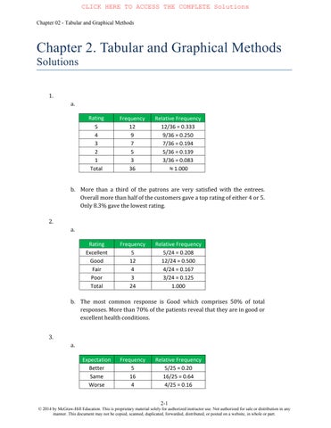
Fromtherelativefrequencydistribution,wecanconcludethatthe majorityoftheevaluationswereeither“OK”or“Horrible”.Noticethat noneoftheresponsesincluded“Outstanding”.Therefore itisnecessary fortheowneroftherestauranttoimprovetheserviceand/orexperience provided.
Thepiechartwhichdepictscategoricaldatainpercentagevalues demonstratesthepoorevaluationsreceived.
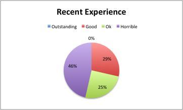
Thebarchartisanotherwaytodepictcategoricaldataeffectively.We noticethatthehighestbarcorrespondstothelastcategory“Horrible” , andthattherearenoresponsesgivenfor“Outstanding.”
Professions Survey
Professions Survey
Thechartsrevealparentpreferences. Sixty-fivepercentofparentswant theirchildrentohaveaprofessionsuchasadoctor,lawyer,bankeror president.Lesspreferableareotherprofessionssuchhumanitarian-aid workeroramoviestar.
b. Since9%ofparentswanttheirchildrentobecomeanathlete,wefind 55 . 9 50.Therefore,among550parentsapproximately50 parentswanttheirkidstobecomeanathlete.
c. Ninefundshadreturnsofatleast0%butlessthan10%;therewere4 fundswithreturnsof10%ormore
d. 12.5%ofthefundshadareturnofatleast10%butnotgreaterthan20%; 95.8%ofthefundshadreturnslessthan20%.
6,166/37,276 = 0.165
7,237/37,276 = 0.194 South 15,501/37,276 = 0.416 West 8,372/37,276 = 0.225 Total = 1.000
19.4%ofpeoplelivingbelowthepovertylevelliveintheMidwestregion.
b.
People Below Poverty Level
25%oftherespondentssaidpayingdowndebtwastheirtopfinancialresolution.
b. Thebarchartshowsthat“Savingmore”isthetopfinancialresolution, followedby“Payingdowndebt”.Onlyasmallportionoftherespondents didn’tknowtheirfinancialresolution. 56. a.
A few days
A few long weekends
One week
Two weeks
0.21(3057) = 642
0.18(3057) = 550
0.36(3057) = 1101
0.25(3057) = 764
Total = 3057
Approximately1101peoplearegoingtotakeaoneweekvacation. b.
58.
Vacation Plan
Use of an unexpected tax refund
Noticethatthemostfrequentresponseswereregardstopayingoffdebtsorputting itinthebank.
b. Since11%of1026respondentssaidtheywouldspendtherefund,we find . 6 3.Therefore,approximately113oftherespondents wouldspendthetaxrefund.
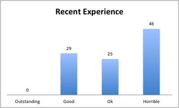
a. Thepiechartisbelow.
b.
ThechartshowsthehighestpercentageofpeopleliveintheSouthand thelowestpercentageliveintheNortheast.
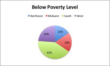
Thechartshowsthehighestpercentageofpeoplelivinginpovertyarein theSouthandthelowestpercentageofpeoplelivinginpovertyareliving intheNortheast.ThepercentageofpeoplelivinginpovertyintheSouth ishigherthanthepercentageofpeoplethatliveinSouth,andthe percentageofpeoplelivinginpovertyintheNortheastislessthanthe percentageofpeoplethatliveintheNortheast.
59. a.
to
to 1750
to
2000 up to 2250 15/60 = 0.250
2250 up to 2500 4/60 =
Total = 1.000
=
b. Themostlikelyattendancerangeisfrom1,750upto2,000witha33% frequency;therewere41timesoutof60thatattendancewaslessthan 2,000.
c. Attendancewasatleast1,750butlessthan2,00033.3%ofthetime; Attendancewaslessthan1,750people35%ofthetime;therefore, attendancewas1,750ormore65%ofthetime.
d. The
Histogram of Attendance in July and August
30 up to 35 10/80 = 0.1250
35 up to 40 7/80 = 0.0875
40 up to 45 3/80 = 0.0375
Total = 1.0000
+ 10 = 70
+ 7 =
= 0.8750
= 0.9625
= 1.0000
b. 60carsgotlessthan30mpg;37.5%ofthecarsgotatleast20butlessthan25mpg; 87.5%ofthecarsgotlessthan35mpg;Since87.5%gotlessthan35mpg,12.5%of thecarsgot35mpgormore
c.
Thedistributionisnotsymmetric;it ispositivelyskewed.
Days Working From Home
62.
a. Therewere4peopleoutof25withanetworthgreaterthan$20billion. Since4/25=0.16,16%ofthewealthiestpeoplehadnetworthgreater than$20billion.
b. Twopeoplehadanetworthlessthan$10billion,whichis2/25=0.08, or8%.Fromthepreviousquestion,weknowthat16%hadanetworth greaterthan$20billion.Therefore,16%+8%=24%didnothaveanet worthbetween$10and$20billion.Consequently,76%hadnetworth between$10billionand$20billion. c.
Thedistributionisnotsymmetric;itisnegativelyskewed.Themajority ofagesrangefromthe60sto70s.Table2.16showsthemajorityofages tobeinthe50sand60s.Further,thisdiagramshowsagesrangingfrom 36to79,whereasTable2.16hasagesrangingfrom36to90. 63.
ThevastmajorityofthePEGratiosfallinthe1range. Thediagram representssomewhatpositivelyskeweddistribution;thereareafew firmswithrelativelyhighPEGratios
Thesechartsshowthatthemajority(60%)ofhouseswereeitherRanch orColonial,butalso40%wereeitherContemporaryorsomeothertype.
b. Tofigureouthowwidetomaketheclasses,findthehighestpriceand subtractthelowestpricetogettherange.Thatis$568,000-$300,000= $268,000.Then,sincewewant7classes,dividetherangeby7; 268,000/7=$38,386 However,foreaseofinterpretation,roundtothe
mostsensiblenumber:$50,000.Therefore,ourclasseswillhaveawidth of$50,000,withalowerboundofthefirstclassof$300,000.
Types of Houses sold in New Jersey
Ogive for House Price
Thehistogramshowsthatthemostfrequenthousepriceisinthe $350,000upto$400,000range.Theogiveshowsthatthemiddleprice (withafrequencyof10/20or50%)isabout$400,000. 65.
ThescatterplotshowsthattherelationbetweenAdvertisingandSalesis positive.Thepositivetrenddemonstratesthatanincreaseinadvertisingwill tendtoincreasesales.
ThescatterplotrevealsnoclearrelationshipbetweenPPGandMPG. CaseStudy2.1:
Thepiechartisbelow.
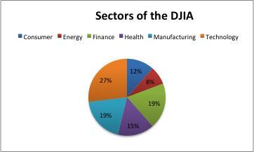
Thesectorswiththelargestrepresentationsarethetechnology,manufacturingand financesectors.Thesectorwiththelowestrepresentationistheenergysector.
CaseStudy2.2
Thenetprofitmarginisafirm’snetprofitaftertaxestorevenue.Itismeasuredin percentage,showingthepercentageofnetincomeperdollarinsalesorother operatingincome.
Histogram for Net Profic Margin
Thedatatendstoclusterbetween0%and10%,asshowninthehistogram.Thenet profitmarginsrangefrom-5.19%to19.95%.Approximately53%ofthefirmshave anetprofitmarginbelow5%.
Histogram for Life Expectancy
Thedatatendstoclusterbetween78and81,asshowninthehistogram. Thedistributionisnegativelyskewed.