Chapter 2
2-1 From Tables A-20, A-21, A-22, and A-24c,
(a) UNS G10200 HR: Sut = 380 (55) MPa (kpsi), Syt = 210 (30) MPa (kpsi) Ans.
(b) SAE 1050 CD: Sut = 690 (100) MPa (kpsi), Syt = 580 (84) MPa (kpsi) Ans.
(c) AISI 1141 Q&T at 540C (1000F): Sut = 896 (130) MPa (kpsi), Syt = 765 (111) MPa (kpsi) Ans.
(d) 2024-T4: Sut = 446 (64.8) MPa (kpsi), Syt = 296 (43.0) MPa (kpsi) Ans.
(e) Ti-6Al-4V annealed: Sut = 900 (130) MPa (kpsi), Syt = 830 (120) MPa (kpsi) Ans.
2-2 (a) Maximize yield strength: Q&T at 425C (800F) Ans.
(b) Maximize elongation: Q&T at 650C (1200F) Ans.
2-3 Conversion of kN/m3 to kg/ m3 multiply by 1(103) / 9.81 = 102
AISI 1018 CD steel: Tables A-20 and A-5 ( ) ( ) 337010 47.4kNm/kg. 76.5102 y S Ans ==
2011-T6 aluminum: Tables A-22 and A-5 ( ) ( ) 316910 62.3kNm/kg. 26.6102
S Ans
Ti-6Al-4V titanium: Tables A-24c and A-5 ( ) ( ) 383010 187kNm/kg. 43.4102 y S Ans
ASTM No. 40 cast iron: Tables A-24a and A-5.Does not have a yield strength. Using the ultimate strength in tension ( )( ) ( ) 342.56.8910 40.7kNm/kg 70.6102
2-4 AISI 1018 CD steel: Table A-5 ( ) ( ) 6 6 30.010 10610in. 0.282 E Ans ==
2011-T6 aluminum: Table A-5 ( ) ( ) 6 6 10.410 10610in. 0.098 E Ans
Ti-6Al-6V titanium: Table A-5 ( ) ( ) 6 6 16.510 10310in. 0.160 E Ans == No. 40 cast iron: Table A-5 ( ) ( ) 6 6 14.510 55.810in. 0.260 E Ans == 2-5 2 2(1) 2 EG GvEv G +==
Using values for E and G from Table A-5, Steel:
The percent difference from the value in Table A-5 is 0.3040.292 0.04114.11percent. 0.292 Ans ==
The percent difference from the value in Table A-5 is 0 percent Ans.
The percent difference from the value in Table A-5 is 0.2860.285 0.003510.351percent. 0.285 Ans == Gray cast iron: ( ) ( ) 14.526.0 0.208. 26.0 vAns ==
The percent difference from the value in Table A-5 is 0.2080.211 0.01421.42percent. 0.211 Ans =−=−
For data in the elastic range, from Eq. (2–2), = (l – l0) / l0 = l / l0 = l / 2
For data in the plastic range, from Eq. (2–8), 0 AA A =
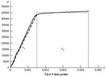
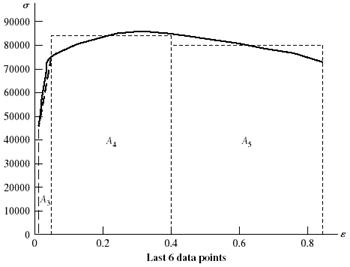
On the next two pages, the data and plots are presented. Figure (a) shows the linear part of the curve from data points 1 to 7. Figure (b) shows data points 1 to 12. Figure (c) shows the complete range Note: The exact value of A0 is used without rounding off.
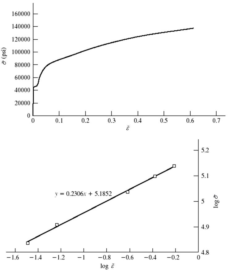
(b) From Fig. (a) the slope of the line from a linear regression is E = 30.5 Mpsi Ans.
From Fig. (b) the equation for the dotted offset line is found to be = 30.5(106) 61 000 (1)
The equation for the line between data points 8 and 9 is = 7.60(105) + 42 900 (2)
Solving Eqs. (1) and (2) simultaneously yields = 45.6 kpsi which is the 0.2 percent offset yield strength. Thus, Sy = 45.6 kpsi Ans.
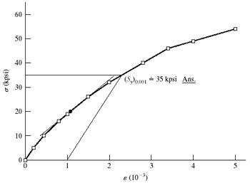
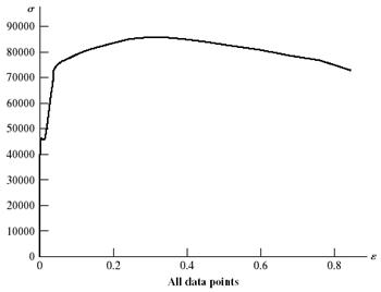
The ultimate strength from Figure (c) is Su = 85.6 kpsi Ans.
The reduction in area is given by Eq. (2-25) as
(a) Linear range
(b) Offset yield
(c) Complete range
(c) The material is ductile since there is a large amount of deformation beyond yield.
(d) The closest material to the values of Sy, Sut, and R is SAE 1045 HR with Sy = 45 kpsi, Sut = 82 kpsi, and R = 40 %. Ans.
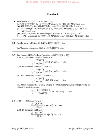
2-7 To plot vs. , the following equations are applied to the data.
Eq. (2-4) P
=
Eq. (2–9)
The results are summarized in the following table and plot. The last 5 points of data are used to plot log vs log .
The curve fit gives m = 0.2306 log 0 = 5.1852 0 = 153.2 kpsi Ans.
The true strain corresponding to 20% cold work is given by Eq. (2–28) as
Eq.(2-30): 153.2(0.2231)108.4kpsi . Eq.(2-32),with 85.6fromProb.2-6, 85.6 107kpsi . 110.2
2-9 W = 0.20, (a) Before cold working: Annealed AISI 1018 steel. Table A-22, Sy = 32 kpsi, Su = 49.5 kpsi, 0 = 90.0 kpsi, m =0.25, f = 1.05 After cold working: Eq. (2-23), 0.25 u m
Lost most of its ductility.
2-10 W = 0.20, (a) Before cold working: AISI 1212 HR steel. Table A-22, Sy = 28 kpsi, Su = 61.5 kpsi, 0 = 110 kpsi, m =0.24, f = 0.85 After cold working: Eq. (2-23), 0.24 u m == Eq. (2-28): 20 11 lnln0.223
(2-30):
Lost most of its ductility
2-11 W = 0.20, (a) Before cold working: 2024-T4 aluminum alloy. Table A-22, Sy = 43.0 kpsi, Su = 64.8 kpsi, 0 = 100 kpsi, m =0.15, f = 0.18
After cold working: Eq. (2-23), 0.15 u m ==
Eq. (2-28): 20
Material fractures. Ans.
2-12 For HB = 275, Eq. (2-36), Su = 3.4(275) = 935 MPa Ans.
2-13 Gray cast iron, HB = 200. Eq. (2-37), Su = 0.23(200) 12.5 = 33.5 kpsi Ans.
From Table A-24, this is probably ASTM No. 30 Gray cast iron Ans.
2-14 Eq. (2-36), 0.5HB = 100 HB = 200 Ans.
2-15 For the data given, converting HB to Su using Eq. (2-36)
(1-6)
(1-7),
2-16 For the data given, converting
2-18, 2-19 These problems are for student research. No standard solutions are provided.
2-20 Appropriate tables: Young’s modulus and Density (Table A-5); 1020 HR and CD (Table A-20); 1040 and 4140 (Table A-21); Aluminum (Table A-24); Titanium (Table A-24c)
Appropriate equations:
Weight/length = A, Cost/length = $/in = ($/lbf) Weight/length, Deflection/length = /L = F/(AE)
With F = 100 kips = 100(103) lbf, Material
The selected materials with minimum values are shaded in the table above. Ans.
2-21 First, try to find the broad category of material (such as in Table A-5). Visual, magnetic, and scratch tests are fast and inexpensive, so should all be done. Results from these three would favor steel, cast iron, or maybe a less common ferrous material. The expectation would likely be hot-rolled steel. If it is desired to confirm this, either a weight or bending test could be done to check density or modulus of elasticity. The weight test is faster. From the measured weight of 7.95 lbf, the unit weight is determined to be
which agrees well with the unit weight of 0.282 lbf/in3 reported in Table A-5 for carbon steel. Nickel steel and stainless steel have similar unit weights, but surface finish and darker coloring do not favor their selection. To select a likely specification from Table A20, perform a Brinell hardness test, then use Eq. (2-36) to estimate an ultimate strength of
0.50.5(200)100 kpsi
uBSH=== . Assuming the material is hot-rolled due to the rough surface finish, appropriate choices from Table A-20 would be one of the higher carbon steels, such as hot-rolled AISI 1050, 1060, or 1080. Ans.
2-22 First, try to find the broad category of material (such as in Table A-5). Visual, magnetic, and scratch tests are fast and inexpensive, so should all be done. Results from these three favor a softer, non-ferrous material like aluminum. If it is desired to confirm this, either a weight or bending test could be done to check density or modulus of elasticity. The weight test is faster. From the measured weight of 2.90 lbf, the unit weight is determined to be
lbf/in
[(1in)/4](36 in)
which agrees reasonably well with the unit weight of 0.098 lbf/in3 reported in Table A-5 for aluminum. No other materials come close to this unit weight, so the material is likely aluminum. Ans.
2-23 First, try to find the broad category of material (such as in Table A-5). Visual, magnetic, and scratch tests are fast and inexpensive, so should all be done. Results from these three favor a softer, non-ferrous copper-based material such as copper, brass, or bronze. To further distinguish the material, either a weight or bending test could be done to check density or modulus of elasticity. The weight test is faster. From the measured weight of 9 lbf, the unit weight is determined to be
[(1in)/4](36 in)
which agrees reasonably well with the unit weight of 0.322 lbf/in3 reported in Table A-5 for copper. Brass is not far off (0.309 lbf/in3), so the deflection test could be used to gain additional insight. From the measured deflection and utilizing the deflection equation for an end-loaded cantilever beam from Table A-9, Young’s modulus is determined to be ( ) ( ) 3 3 4 10024 17.7Mpsi 3 3(1)64(17/32)
which agrees better with the modulus for copper (17.2 Mpsi) than with brass (15.4 Mpsi). The conclusion is that the material is likely copper. Ans.
2-24 This problem is for student research. No standard solution is provided.
2-25 For strength, = F/A = S A = F/S For mass, m = Al= (F/S) l
Thus, f 3(M ) = /S , and maximize S/ ( = 1)
In Fig. (2-27), draw lines parallel to S/
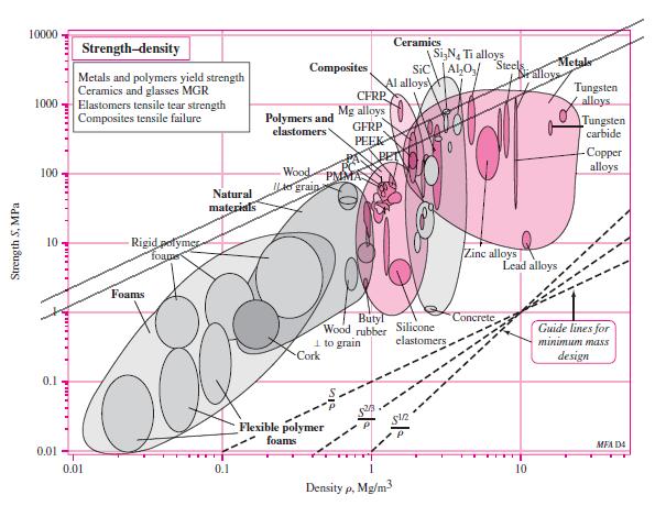
The higher strength aluminum alloys have the greatest potential, as determined by comparing each material’s bubble to the S/guidelines. Ans.
2-26 For stiffness, k = AE/l A = kl/E
For mass, m = Al= (kl/E) l=kl2 /E
Thus, f 3(M) = /E , and maximize E/ ( = 1)
In Fig. (2-24), draw lines parallel to E/
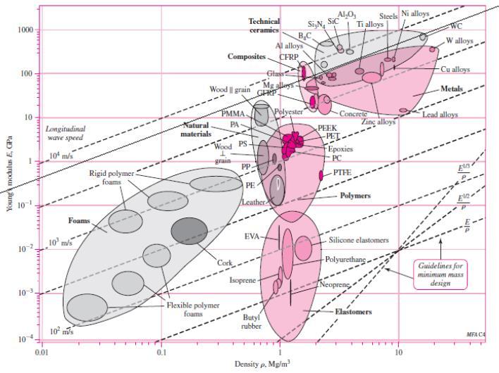
From the list of materials given, tungsten carbide (WC) is best, closely followed by aluminum alloys. They are close enough that other factors, like cost or availability, would likely dictate the best choice. Polycarbonate polymer is clearly not a good choice compared to the other candidate materials. Ans
2-27 For strength, = Fl/Z = S (1)
where Fl is the bending moment and Z is the section modulus [see Eq. (3-26b)]. The section modulus is strictly a function of the dimensions of the cross section and has the units in3 (ips) or m3 (SI). Thus, for a given cross section, Z =C (A)3/2, where C is a number. For example, for a circular cross section, C = ( ) 1 4 . Then, for strength, Eq. (1) is
For mass, 2/32/3 5/3 2/3
Thus, f 3(M) = /S 2/3, and maximize S 2/3/ (= 2/3)
In Fig. (2-27), draw lines parallel to S 2/3/
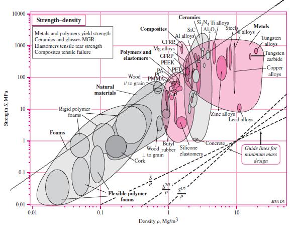
From the list of materials given, a higher strength aluminum alloy has the greatest potential, followed closely by high carbon heat-treated steel. Tungsten carbide is clearly not a good choice compared to the other candidate materials. .Ans.
2-28 Equation (2-41) applies to a circular cross section. However, for any cross section shape it can be shown that I = CA 2, where C is a constant. For example, consider a rectangular section of height h and width b, where for a given scaled shape, h = cb, where c is a constant. The moment of inertia is I = bh 3/12, and the area is A = bh. Then I = h(bh2)/12 = cb (bh2)/12 = (c/12)(bh)2 = CA 2, where C = c/12 (a constant). Thus, Eq. (2-42) becomes
and Eq. (2-44) becomes
Thus, minimize ( ) 3
. From Fig. (2-24)
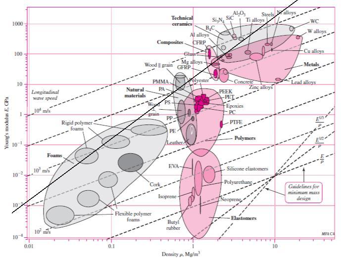
From the list of materials given, aluminum alloys are clearly the best followed by steels and tungsten carbide. Polycarbonate polymer is not a good choice compared to the other candidate materials. Ans.
2-29 For stiffness, k = AE/l A = kl/E For mass, m = Al= (kl/E) l=kl2 /E
So, f 3(M) = /E, and maximize E/. Thus, = 1. Ans.
2-30 For strength, = F/A = S A = F/S
For mass, m = Al= (F/S) l
So, f 3(M ) = /S, and maximize S/. Thus, = 1. Ans.
2-31 Equation (2-41) applies to a circular cross section. However, for any cross section shape it can be shown that I = CA 2, where C is a constant. For the circular cross section, C = (4) 1 [see Eq. (2-41)]. Another example, consider a rectangular section of height h and width b, where for a given scaled shape, h = cb, where c is a constant. The moment of inertia is I = bh 3/12, and the area is A = bh. Then I = h(bh2)/12 = cb (bh2)/12 = (c/12)(bh)2 = CA 2 , where C = c/12, a constant
Thus, Eq. (2-42) becomes
and Eq. (2-44) becomes
So, minimize ( ) 3 1/2 fM E = , or maximize
2-32 For strength,
= . Thus, = 1/2. Ans.
= Fl/Z = S (1)
where Fl is the bending moment and Z is the section modulus [see Eq. (3-26b)]. The section modulus is strictly a function of the dimensions of the cross section and has the units in3 (ips) or m3 (SI). The area of the cross section has the units in2 or m2 . Thus, for a given cross section, Z =C (A)3/2, where C is a number. For example, for a circular cross section, Z = d 3/(32)and the area is A = d 2/4. This leads to C =( ) 1 4 So, with Z =C (A)3/2, for strength, Eq. (1) is 2/3 3/2
mass, 2/32/3 5/3 2/3
So, f 3(M) = /S 2/3, and maximize S 2/3/. Thus, = 2/3. Ans.
2-33 For stiffness, k=AE/l, or, A = kl/E.
Thus, m = Al =(kl/E )l = kl 2 /E. Then, M = E /and = 1.
From Fig. 2-24, lines parallel to E / for ductile materials include steel, titanium, molybdenum, aluminum alloys, and composites.
For strength, S = F/A, or, A = F/S.
Thus, m = Al =F/Sl = Fl /S. Then, M = S/ and = 1.
From Fig. 2-27, lines parallel to S/ give for ductile materials, steel, aluminum alloys, nickel alloys, titanium, and composites.
Common to both stiffness and strength are steel, titanium, aluminum alloys, and composites. Ans.
2-34 See Prob. 1-13 solution for x = 122.9 kcycles and x s = 30.3 kcycles. Also, in that solution it is observed that the number of instances less than 115 kcycles predicted by the normal distribution is 27; whereas, the data indicates the number to be 31.
From Eq. (1-4), the probability density function (PDF), with x = and ˆ x s = , is
The discrete PDF is given by f /(Nw), where N = 69 and w = 10 kcycles. From the Eq. (1) and the data of Prob. 1-13, the following plots are obtained.
2 0.002898551 0.001526493
1 0.001449275 0.002868043
3 0.004347826 0.004832507
5 0.007246377 0.007302224
8 0.011594203 0.009895407
12 0.017391304 0.012025636
6 0.008695652 0.013106245
10 0.014492754 0.012809861
8 0.011594203 0.011228104
5 0.007246377 0.008826008
2 0.002898551 0.006221829
3 0.004347826 0.003933396
2 0.002898551 0.002230043
1 0.001449275 0.00021141
Plots of the PDF’s are shown below.
It can be seen that the data is not perfectly normal and is skewed to the left indicating that the number of instances below 115 kcycles for the data (31) would be higher than the hypothetical normal distribution (27).