CHAPTER 2
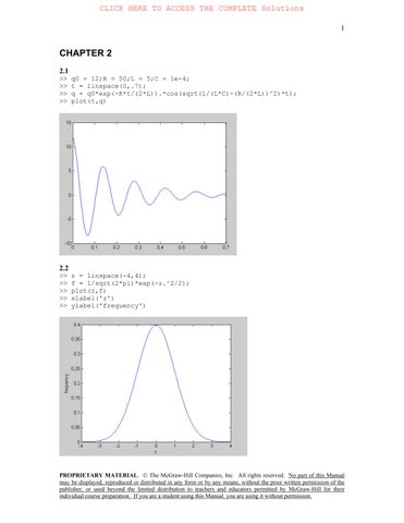
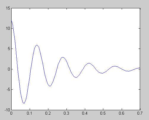
2.1
>> q0 = 12;R = 50;L = 5;C = 1e-4; >> t = linspace(0,.7);
>> q = q0*exp(-R*t/(2*L)).*cos(sqrt(1/(L*C)-(R/(2*L))^2)*t);
>> plot(t,q)
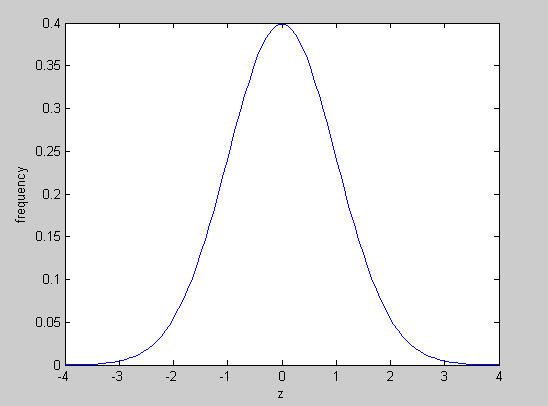
2.2
>> z = linspace(-4,4);
>> f = 1/sqrt(2*pi)*exp(-z.^2/2);
>> plot(z,f)
>> xlabel('z')
>> ylabel('frequency')
PROPRIETARY MATERIAL. © The McGraw-Hill Companies, Inc. All rights reserved. No part of this Manual may be displayed, reproduced or distributed in any form or by any means, without the prior written permission of the publisher, or used beyond the limited distribution to teachers and educators permitted by McGraw-Hill for their individual course preparation. If you are a student using this Manual, you are using it without permission.
2.3 (a)
>> t = linspace(5,29,5)
t = 5 11 17 23 29
(b)
>> x = linspace(-3,4,8)
x = -3 -2 -1 0 1 2 3 4
2.4 (a)
>> v = -3:0.5:1
v =
(b)
>> r = 8:-0.5:0
r =
Columns 1 through 6
Columns 7 through 12
Columns 13 through 17 2.0000 1.5000
2.5
>> F = [11 12 15 9 12];
>> x = [0.013 0.020 0.009 0.010 0.012];
>> k = F./x
k = 1.0e+003 *
>> U = .5*k.*x.^2
U =
>> max(U)
ans = 0.1200
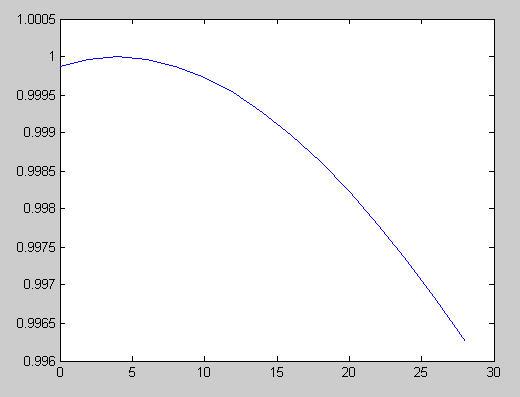
2.6
>> TF = 32:3.6:82.4; >> TC = 5/9*(TF-32); >> rho = 5.5289e-8*TC.^3-8.5016e-6*TC.^2+6.5622e-5*TC+0.99987; >> plot(TC,rho)
PROPRIETARY MATERIAL. © The McGraw-Hill Companies, Inc. All rights reserved. No part of this Manual may be displayed, reproduced or distributed in any form or by any means, without the prior written permission of the publisher, or used beyond the limited distribution to teachers and educators permitted by McGraw-Hill for their individual course preparation. If you are a student using this Manual, you are using it without permission.
2.7
>> A = [.035 .0001 10 2;
0.02 0.0002 8 1;
0.015 0.001 19 1.5;
0.03 0.0008 24 3;
0.022 0.0003 15 2.5]
A = 0.0350 0.0001
>> U = sqrt(A(:,2))./A(:,1).*(A(:,3).*A(:,4)./(A(:,3)+2*A(:,4))).^(2/3)
U = 0.3624 0.6094 2.5053 1.6900 1.1971
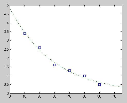
2.8
>> t = 10:10:60; >> c = [3.4 2.6 1.6 1.3 1.0 0.5]; >> tf = 0:75; >> cf = 4.84*exp(-0.034*tf); >> plot(t,c,'s',tf,cf,':') >> xlim([0 75])
PROPRIETARY MATERIAL. © The McGraw-Hill Companies, Inc. All rights reserved. No part of this Manual may be displayed, reproduced or distributed in any form or by any means, without the prior written permission of the publisher, or used beyond the limited distribution to teachers and educators permitted by McGraw-Hill for their individual course preparation. If you are a student using this Manual, you are using it without permission.
2.9
>> t = 10:10:60;
>> c = [3.4 2.6 1.6 1.3 1.0 0.5];
>> tf = 0:70;
>> cf = 4.84*exp(-0.034*tf); >> semilogy(t,c,'s',tf,cf,'--')
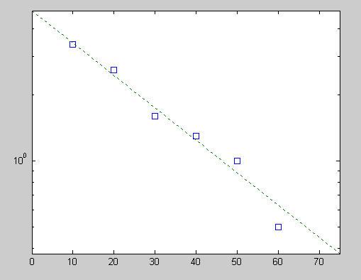
log034.084.4loglog =
The result is a straight line. The reason for this outcome can be understood by taking the common logarithm of the function to give, et c 10 10 10
Because log10e = 0.4343, this simplifies to the equation for a straight line,
PROPRIETARY MATERIAL. © The McGraw-Hill Companies, Inc. All rights reserved. No part of this Manual may be displayed, reproduced or distributed in any form or by any means, without the prior written permission of the publisher, or used beyond the limited distribution to teachers and educators permitted by McGraw-Hill for their individual course preparation. If you are a student using this Manual, you are using it without permission.
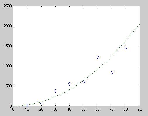
2.10
>> v = 10:10:80;
>> F = [25 70 380 550 610 1220 830 1450];
>> vf = 0:90;
>> Ff = 0.2741*vf.^1.9842; >> plot(v,F,'d',vf,Ff,':')
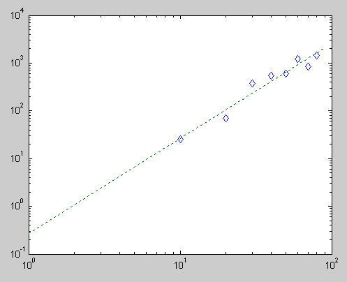
2.11
>> v = 10:10:80;
>> F = [25 70 380 550 610 1220 830 1450];
>> vf = 0:90;
>> Ff = 0.2741*vf.^1.9842;
>> loglog(v,F,'d',vf,Ff,':')
PROPRIETARY MATERIAL. © The McGraw-Hill Companies, Inc. All rights reserved. No part of this Manual may be displayed, reproduced or distributed in any form or by any means, without the prior written permission of the publisher, or used beyond the limited distribution to teachers and educators permitted by McGraw-Hill for their individual course preparation. If you are a student using this Manual, you are using it without permission.
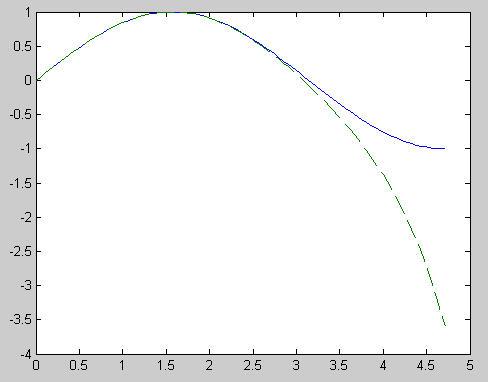
2.12
>> x = linspace(0,3*pi/2);
>> s = sin(x);
>> sf = x-x.^3/factorial(3)+x.^5/factorial(5)-x.^7/factorial(7);
>> plot(x,s,x,sf,'--')
2.13 (a)
>> m=[83.6
>> vt=[53.4
>> g=9.81; rho=1.225;
>> A=[0.454 0.401 0.453 0.485 0.532 0.474 0.486];
>> cd=g*m./vt.^2;
>> CD=2*cd/rho./A
PROPRIETARY MATERIAL. © The McGraw-Hill Companies, Inc. All rights reserved. No part of this Manual may be displayed, reproduced or distributed in any form or by any means, without the prior written permission of the publisher, or used beyond the limited distribution to teachers and educators permitted by McGraw-Hill for their individual course preparation. If you are a student using this Manual, you are using it without permission.
CD = 1.0343
(b)
>> CDavg=mean(CD),CDmin=min(CD),CDmax=max(CD)
CDavg = 0.9943
CDmin = 0.9591
CDmax = 1.0343
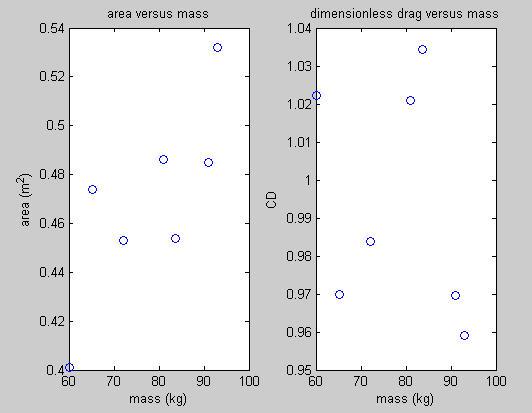
(b)
>> subplot(1,2,1);plot(m,A,'o')
>> xlabel('mass (kg)');ylabel('area (m^2)') >> title('area versus mass') >> subplot(1,2,2);plot(m,CD,'o') >> xlabel('mass (kg)');ylabel('CD') >> title('dimensionless drag versus mass')
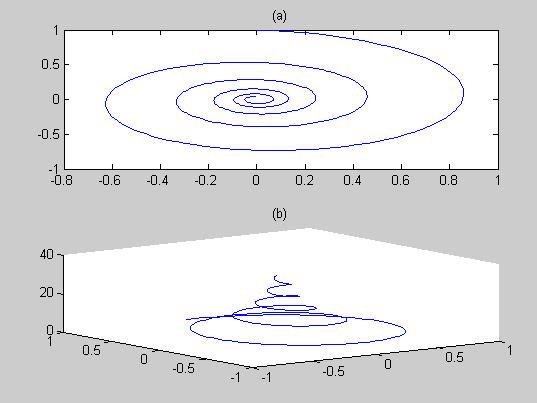
2.14 (a)
t = 0:pi/50:10*pi; subplot(2,1,1);plot(exp(-0.1*t).*sin(t),exp(-0.1*t).*cos(t)) title('(a)') subplot(2,1,2);plot3(exp(-0.1*t).*sin(t),exp(-0.1*t).*cos(t),t); title('(b)')
PROPRIETARY MATERIAL. © The McGraw-Hill Companies, Inc. All rights reserved. No part of this Manual may be displayed, reproduced or distributed in any form or by any means, without the prior written permission of the publisher, or used beyond the limited distribution to teachers and educators permitted by McGraw-Hill for their individual course preparation. If you are a student using this Manual, you are using it without permission.
2.15 (a)
>> x = 2; >> x ^ 3;
>> y = 8 - x y = 6 (b)
>> q = 4:2:10;
>> r = [7 8 4; 3 6 -2];
>> sum(q) * r(2, 3)
ans = -56
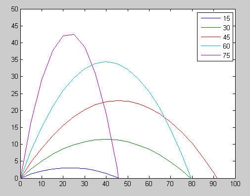
2.16
>> y0=0;v0=30;g=9.81; >> x=0:5:100; >> theta0=15*pi/180; >> y1=tan(theta0)*x-g/(2*v0^2*cos(theta0)^2)*x.^2+y0; >> theta0=30*pi/180;
>> y2=tan(theta0)*x-g/(2*v0^2*cos(theta0)^2)*x.^2+y0; >> theta0=45*pi/180;
>> y3=tan(theta0)*x-g/(2*v0^2*cos(theta0)^2)*x.^2+y0; >> theta0=60*pi/180;
>> y4=tan(theta0)*x-g/(2*v0^2*cos(theta0)^2)*x.^2+y0; >> theta0=75*pi/180;
>> y5=tan(theta0)*x-g/(2*v0^2*cos(theta0)^2)*x.^2+y0; >> y=[y1' y2' y3' y4' y5']
>> plot(x,y)
>> axis([0 100 0 50])
>> legend('15','30','45','60','75')
PROPRIETARY MATERIAL. © The McGraw-Hill Companies, Inc. All rights reserved. No part of this Manual may be displayed, reproduced or distributed in any form or by any means, without the prior written permission of the publisher, or used beyond the limited distribution to teachers and educators permitted by McGraw-Hill for their individual course preparation. If you are a student using this Manual, you are using it without permission.
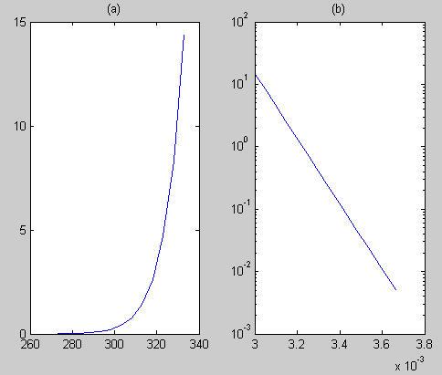
2.17
>> R=8.314;E=1e5;A=7E16; >> Ta=273:5:333; >> k=A*exp(-E./(R*Ta))
k = Columns 1 through 10
Columns 11 through 13
>> subplot(1,2,1);plot(Ta,k)
>> subplot(1,2,2);semilogy(1./Ta,k)
PROPRIETARY MATERIAL. © The McGraw-Hill Companies, Inc. All rights reserved. No part of this Manual may be displayed, reproduced or distributed in any form or by any means, without the prior written permission of the publisher, or used beyond the limited distribution to teachers and educators permitted by McGraw-Hill for their individual course preparation. If you are a student using this Manual, you are using it without permission.
The result in (b) is a straight line. The reason for this outcome can be understood by taking the common logarithm of the function to give,
Thus, a plot of log10k versus 1/Ta is linear with a slope of –(E/R)log10e = –5.2237×10³ and an intercept of log10A = 16.8451.
PROPRIETARY MATERIAL. © The McGraw-Hill Companies, Inc. All rights reserved. No part of this Manual may be displayed, reproduced or distributed in any form or by any means, without the prior written permission of the publisher, or used beyond the limited distribution to teachers and educators permitted by McGraw-Hill for their individual course preparation. If you are a student using this Manual, you are using it without permission.