7 Correlation Analysis
Learning Objectives
By the end of this chapter, you will be able to understand:
Introduction
Meaning and computation of covariance
Application of covariance
Limitations of covariance
Meaning and signi cance of correlation
Types of correlation
Correlation v. Causation
Correlation v. Covariance
Techniques for measuring correlation
Graphic Method - Scatter Diagram
Algebraic Methods
Karl Pearson’s coef cient of correlation
Properties of Correlation
Computation of coef cient of correlation
Limitations of Karl Pearson’s coef cient of correlation
Coef cient of determination
Probable and standard errors
Probable error of coef cient of correlation
Standard error of coef cient of correlation
Spearman’s rank correlation
Solved Examples
362
Exercises
UNIT III : SIMPLE CORRELATION AND REGRESSION ANALYSIS
Short Questions
Long Questions
Numerical Questions
Key Formulas
7.1
INTRODUCTION
Correlation is the statistical measure that is used for determining the degree to which two variables are related or the degree to which they co-vary. It enables us to know whether the two variables are associated with each other and to what extent or not.
We know that the circumference of a circle is measured as 2 r. It implies that the radius and circumference are correlated. As the radius increases, the circumference goes up. In other words, a higher circumference is associated with a higher radius of a circle. The relationship is mathematical and given by a fixed formula. What about the height and weight of a group of people? Generally, taller persons have higher weight compared to shorter ones. It is not possible to determine the exact weight of a person from his height or vice–versa. Special statistical techniques have been developed to examine the existence of statistical relationships between bivariate paired data sets. One such technique that applies to quantitative data sets is Correlation Analysis. The present chapter discusses two important measures of association viz., covariance and correlation. Covariance is a numerical measure that reveals the direction of the linear relationship between two variables. Correlation analysis is a means for examining such relationships systematically. It indicates whether there is any relationship between any two given variables, if yes, then it reflects the direction of the relationship and the strength of the same.
In the next section, we will delve into the concept of covariance that lays the groundwork for comprehending Pearson’s coefficient. Furthermore, we will explore the various aspects of the interpretation of the covariance between two variables and its relevance in business and economic research and analysis. We will also examine its inherent limitations, due to which correlation is preferred as a measure of association.
7.2 MEANING AND COMPUTATION OF COVARIANCE
Covariance is a statistical measure that indicates the extent to which two variables change together. It is a measure of the directional relationship between two random variables, denoted as X and Y. Covariance may be positive, negative or zero. While positive covariance indicates that as one variable increases, the other tends to increase as well, negative covariance indicates that as one variable increases, the other tends to decrease and zero covariance implies no linear relationship between the variables. The magnitude of covariance is not easy to interpret directly because it is not standardised. That is, it depends on the scales of the variables involved. However, a larger covariance (in absolute terms) implies a stronger relationship between the variables.
Formula and Interpretation of Covariance:
Covariance of X and Y denoted as Cov(X,Y) or xy is computed as:
Cov(X, Y) = NN XXYYXXYYXXYY N 1122 ()()()()...()() −−+−−++−−
where XY XY NN , == ∑∑ , x = XX and y = YY are the deviations of ith value of X and Y from their respective arithmetic mean.
The alternate formula for the calculation of covariance is: XYXY CovXY NNN (,) =−
The value of the covariance between two variables provides insights into the following aspects of their association:
1. Direction of Relationship: Covariance indicates the directional relationship between two random variables. It can be positive, negative, or zero.
2. Magnitude of Relationship: The magnitude of covariance is not easy to interpret directly because it is not normalized. It can take a value between – to depending on the scales of the variables involved. However, a larger covariance (in absolute terms) implies a stronger relationship between the variables.
3. Scale Dependence: Covariance is sensitive to the scale of the variables. It can be difficult to interpret because its value depends on the units of the variables. If Cov(X, Y) is the covariance between variables X and Y and the variables are changed to aXb + and cYd + then CovaXbcYd (,) ++ = a × c. Cov(X, Y) where a, b, c, d are arbitrary constants.
7.2.1 A pplication of Covariance
Covariance has significant applications across various fields, helping in identifying patterns, making predictions and informed decisions. Its relevance in portfolio management, market analysis, risk management, and marketing research provides valuable insights for business decision-making. In finance, for example, covariance is crucial in portfolio theory for constructing diversified portfolios. It helps in understanding the relationship between the returns of different securities or assets and market indices.
A positive covariance between a stock and a market index indicates that the stock tends to move in the same direction as the market. Conversely, a negative covariance suggests it moves in the opposite direction. By analysing these relationships, investors can optimise their portfolios to trade off risk and return effectively.
In market analysis, covariance can reveal how different economic indicators move together, assisting analysts in predicting future market trends. It can identify the relationship between different variables, such as consumer behaviour and sales, enabling more targeted and effective marketing strategies.
Example 7.1: An investor advisor has forecasted the returns on securities A and B for the period from January to October as given below:
364 UNIT III : SIMPLE CORRELATION AND REGRESSION ANALYSIS
Calculate the covariance between the two and interpret the result.
Solution:
To calculate the covariance between the returns on securities A and B, we assign X and Y variables to ‘Return on A’ and ‘Return on B’ respectively. Let, the number of pairs of data be N. Since data is available for ten months, therefore, N = 10.
The formula for covariance to be used is: xy CovXY N (,) = ∑ where, XY XY NN , ==
, x = X and y = YY . We would prepare a table by following the steps for the required computation.
Steps: 1. Calculate the mean return for each security.
2. Determine the deviation of each return from its respective mean.
3. Multiply the deviations of corresponding returns for X and Y.
4. Calculate the average of these products.
Computation of Covariance Between Returns of Securities X and Y
Alternatively,
= 401.2 – 400 = 1.2
Interpretation: The covariance between the returns on security A and security B is 1.2. This positive covariance indicates that the returns on securities A and B tend to move in the same direction. When the return on Security A increases, the return on Security B also tends to increase, and vice versa. However, since covariance is not standardized, this value alone does not indicate the strength of the relationship between the returns.
7.2.2 Limitations of Covariance
While covariance is a valuable tool in business statistics for analysing relationships between variables, it has a limitation that it is difficult to interpret because it is sensitive to the units of measurement, making it complicated to compare covariances across different datasets or variables measured in different units. Besides, it does not indicate the strength of the relationship. Since it does not provide a standardized measure of association, it is challenging to determine whether the covariance represents a strong or weak relationship between variables.
Another measure of association for easier interpretation is the correlation coefficient which describes both the direction and the strength of the linear relationship between two variables. The next section elaborates on the concept of correlation.
In statistics, an association is any relationship between two measured quantities that renders them statistically dependent. The term “association” refers broadly to any such relationship, whereas the narrower term “correlation” refers to a linear relationship between two quantities. In quantitative research, the term “association” is often used to emphasize that a relationship being discussed is not necessarily causal (or correlation does not necessarily imply causation). Many statistical measures of association can be used to infer the presence or absence of an association in a sample of data. Correlation Analysis is a statistical technique that is used to examine the strength and direction of the relationship between two quantitative variables. However, it measures covariation and not causation. Correlation does not imply cause and effect relation. The magnitude of the coefficient of correlation indicates the strength while its sign reveals the direction of the relationship between the variables. The strength of the relationship is based on the closeness of the points, representing a pair of values of two variables that are plotted on a graph to a straight line that is drawn over such point as best fit. This straight line is used as a frame of reference for evaluating the relationship.
The correlation between two variables X and Y implies that with the change in the value of one variable in a particular direction, the value of the other variable changes either in the same direction (i.e. positively) or in the opposite direction (i.e. negatively). The value of the correlation varies from 1 to –1. Correlation value 1 implies a perfect positive correlation, 0 indicates no correlation and –1 is a perfect negative correlation. It is assumed
III : SIMPLE CORRELATION AND REGRESSION ANALYSIS
to be linear, i.e. the relative movement of the two variables can be represented by drawing a straight line on graph paper.
The coefficient of correlation does not have any units. It is a dimensionless value that measures the strength and direction of the linear relationship between two variables. Therefore, it would be inaccurate to say that the coefficient of correlation must be in the same units as the original data. As already mentioned, the correlation coefficient ranges between 1 and 1. A positive value of r indicates a positive linear relationship between the variables, while a negative value indicates a negative linear relationship. The magnitude of r represents the strength of the relationship, with values closer to 1 or 1 indicating a stronger linear relationship. Since the correlation coefficient is a unitless value, it is not influenced by the units of measurement used for the variables. Thus, the coefficient will remain the same irrespective of the unit of measurement of the variables i.e., inches, kilograms, rupees, etc. The correlation coefficients from different studies or data sets are comparable even if they use different units of measurement for their variables.
According to L.R. Connor, “If two or more quantities vary in sympathy so that movements in one tend to be accompanied by corresponding movements in others, then they are said to be correlated.” Similarly, Croxton and Cowden define correlation as “the relationship of quantitative nature. The appropriate tool for discovering and measuring the relationship and expressing it in the brief formula is known as correlation”. Conceptually, correlation is a statistical tool used to study the relationship between two variables.
Correlation analysis involves various methods and techniques to examine and quantify the extent of this relationship. The degree of this relationship is often represented by the coefficient of correlation, denoted by r or (x, y). Correlation is essential for measuring the degree of relationship between different variables in both physical and social sciences.
For instance, economists use correlation to study relationships between variables such as demand and supply, selling price and output, GDP and inflation rates, and income and consumption. For instance, an increase in advertisement expenditure is likely to increase sales, while an increase in the price of a product typically decreases demand.
Moreover, correlation analysis is a vital tool in market surveys and research, helping in the development of effective strategies. By understanding the relationships between various factors, businesses and researchers can make more informed decisions. For example, businesses can optimize their marketing efforts by understanding the correlation between advertising expenditure and sales growth. Economists can predict economic trends by analysing the correlation between GDP and inflation rates. These relationships can be linear or curvilinear and form the basis for the concept of regression.
The significance of correlation lies in its ability to quantify and describe the relationship between two variables. Its importance can be highlighted by the following points:
(i) Quanti es Relationships: Correlation provides a numerical value that expresses the strength and direction of the relationship between two variables. This helps in understanding how closely related the variables are.
(ii) Predictive Power: A strong correlation between two variables can be used to make predictions. For example, if there is a strong positive correlation between advertising expenditure and sales, future sales can be estimated based on planned advertising budgets.
(iii) Identi es Patterns: Correlation helps in identifying patterns and trends in data. By analysing the relationship between variables, one can uncover underlying patterns that might not be immediately obvious.
(iv) Basis for Regression Analysis: Correlation is the foundation for regression analysis, which involves predicting the value of a dependent variable based on the value of one or more independent variables. Understanding the correlation helps in building accurate regression models.
(v) Provides Information for Decisions: In business, economics, and social sciences, correlation analysis helps in informed decision-making by providing insights into how variables interact. For example, understanding the correlation between market trends and sales can help strategic sales planning.
(vi) Evaluates Consistency: In research, correlation is used to evaluate the consistency and reliability of measurements. A high correlation between different tests or measurements indicates reliable and consistent results.
(vii) Assesses Risk and Relationships in Finance: In nance, correlation is used to assess the relationships between different securities. Understanding these relationships helps in portfolio diversi cation and risk management.
(viii) Supports Hypothesis Testing: Correlation analysis is often used in hypothesis testing to determine whether there is a signi cant relationship between variables. This is crucial for scienti c research and the validation of theories.
Thus, correlation is a powerful tool in both physical and social sciences for analysing relationships between variables. Whether the relationship is linear or curvilinear, understanding these correlations helps researchers and analysts make informed decisions, predict future trends, and develop effective strategies. It helps to understand complex data and derive meaningful conclusions from their analyses. In the upcoming section, we delve into the nuances of correlation by exploring different types of relationships between related variables.
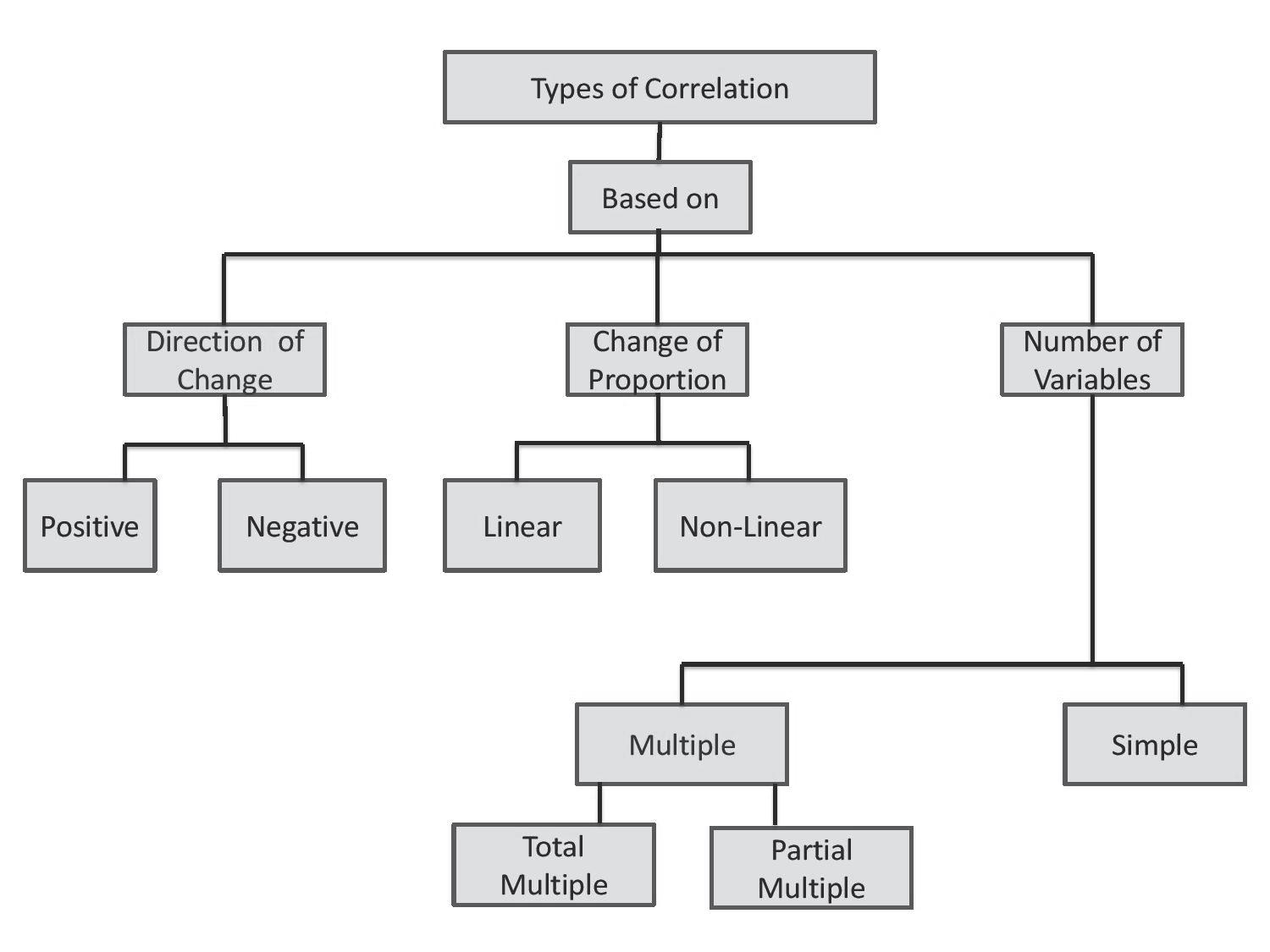
7.4 TYPES OF CORRELATION
As highlighted in the preceding sections, correlation serves as a statistical measure that describes the relationship between two variables. It indicates how variations in one variable correspond to changes in another. Correlation can manifest as positive, negative, or zero, depending upon the direction and strength of the relationship. Accordingly, correlation may be categorised into the following four types:
(a) Positive and negative.
(b) Linear and non–linear.
(c) Simple and Multiple.
(d) Partial and total.
Let us explore the meaning and distinct features of these different types of correlation. (a) Positive and Negative Correlation: The most commonly used classi cation of correlation is negative and positive correlation, depending on the direction of change of the variables. Suppose two variables tend to move together in the same direction, meaning an increase in the value of one variable is accompanied by an increase in the value of the other or a decrease in the value of one variable is accompanied by a decrease in the value of the other. In that case, the correlation is called positive or direct correlation. A correlation coef cient of +1 signi es a perfect positive correlation. Thus, a positive correlation occurs when the variables move together in the same direction. For instance, when income rises, consumption also rises, and when income falls, consumption also falls. This implies that there is a positive correlation between income and consumption. Similarly, the expenditure on advertising and the sales (units) of a product may exhibit a positive correlation, as demonstrated by the following data.
A negative correlation between two variables means that as the value of one variable increases, the value of the other variable tends to decrease. Conversely, as the value of one variable decreases, the value of the other variable tends to increase. This indicates an inverse relationship between the two variables. The strength of the negative correlation is determined by the degree to which the variables move in opposite directions. For example, as the price of a commodity decreases, its demand typically rises, and conversely, when the price increases, demand tends to decrease. Consequently, a negative correlation exists between the price and demand for a commodity, as demonstrated by the following data.
Price (`) 8 9 10 11 12 13 14 15 16 17
Thus, correlation is negative when the two variables move in opposite directions. If two variables consistently move in opposite directions, such that an increase or decrease in one variable corresponds with a decrease or increase in the other variable, this relationship is termed a negative or inverse correlation. A correlation coefficient of –1 signifies a perfect negative correlation.
(
b) Linear and Non–linear (Curvilinear) Correlation: Linear correlation describes a relationship between two variables where the change in one variable is directly proportional to the change in the other, meaning that the alteration in one variable corresponds to the change in another variable in a constant ratio. When represented graphically, this relationship forms a straight–line pattern. In economics, there is often a linear relationship between income and expenditure. For example, if the income of an individual increases from `10,000 to `20,000 per month, his expenditure may increase from `8,000 to `16,000, exhibiting a linear pattern.
Non–linear or curvilinear correlation refers to a relationship between two variables that cannot be accurately represented by a straight line. Instead, the relationship may exhibit a curved or non–linear pattern when plotted on a graph. Thus, in a curvilinear correlation, the change in one variable does not follow a constant ratio with the change in another variable. For example, the relationship between interest rates and investment may exhibit a curvilinear pattern. Initially, as interest rates decrease, investment tends to increase due to lower borrowing costs. However, beyond a certain point, further decreases in interest rates may have diminishing returns on investment, leading to a curvilinear pattern.
(
c) Simple and Multiple Correlation: When only two variables are studied, the relationship is a simple or bivariate correlation. For example, the correlation between the price and quantity demanded of a product, quantity of money and price level, employee satisfaction and productivity, etc.
Multiple correlation examines the relationship between two or more variables simultaneously. For example, the correlation between price of a product, quantity demanded, income level and price of a related commodity. Similarly, multi-correlation analysis examines the relationship between product quality, advertisement expenditure, customer service, and price of a product.
(
d) Partial and Total correlation: In the case of multiple correlation, we have two options: to either study partial correlation or examine the total correlation. Partial correlation measures the strength and direction of the relationship between two variables while keeping constant one or more additional variables. For example, employee satisfaction, employee productivity, and company profitability are correlated variables. In partial correlation analysis, employee productivity is held constant to understand the relationship between employee satisfaction and company profitability. Similarly, to understand the effectiveness of advertising campaigns, we may analyze the correlation between advertising spending and product sales, while keeping the impact of brand awareness constant. Another example is determining the correlation between stock prices and earnings of a company while keeping the market volatility constant. Thus, in partial correlation we consider only two variables influencing each other while the effect of one or more variable(s) is held constant. In multiple correlation analysis, the total correlation examines the combined effect of the partial correlations between the various related variables. For example, it
370
UNIT III : SIMPLE CORRELATION AND REGRESSION ANALYSIS
helps in understanding the interplay among variables such as employee workload, work environment, and employee satisfaction.
The preceding paragraphs delineated different types of correlation. Understanding these various types of correlation enables researchers and analysts to identify intricate patterns within datasets, thereby facilitating more sophisticated interpretations and informed decision–making processes. This helps us to gain deeper insights into the multifaceted nature of relationships between variables across diverse domains. In the present chapter, our focus will be directed towards simple and linear correlations. It is a common mistake that correlation is misinterpreted as implying a cause–and–effect relationship or causation. However, this assumption is incorrect. Next, we address this prevalent misconception regarding correlation and causation.
7.5 CORRELATION v. CAUSATION
Correlation is not causation. Correlation is a measure of the relationship between two variables. Two variables are considered to be statistically related, if the value of one variable increases or decreases and so does the value of the other variable. However, it does not imply a cause-and-effect relationship among the variables.
The coefficient of correlation is a number describing the relative change in one variable when there is a change in the other. It describes the size and direction of a relationship between the two variables. Its value lies between -1 and +1. A correlation coefficient of +1 implies a strong positive relationship between two sets of numbers, –1 implies a strong negative relationship and 0 implies no relationship whatsoever. However, it does not automatically mean that the change in one variable is the cause of the change in the values of the other variable.
“Correlation is not causation”. It means that just because two variables correlate does not necessarily mean that one causes the other. However, if a correlation exists then it may guide the statistician or researcher to further investigate whether one variable causes the other. Causation indicates that the occurrence of one event is the result of the occurrence of the other event, referred to as cause and effect. For example, just because Indian people tend to spend more in the shops when the weather is cold and less when it is hot does not mean that the cold weather causes high spending. A more plausible explanation would be that cold weather tends to coincide with Diwali and New Year sales.
Reasons for correlation not being causation:
Correlation between two variables may be caused by a third factor that affects both of them called a confounder or confounding variable.
The relationship between two variables may be coincidental. The two variables may not be related at all but they correlate by chance.
The two variables may have bidirectional causations on one another and there may not exist a cause–and–effect relationship between the two.
There may exist a spurious or nonsensical correlation between two variables that may seem to be a causal relationship.
7.6 CORRELATION v. COVARIANCE
Covariance and correlation are both measures of the association between two variables, but they differ in their approach to quantifying and interpreting this relationship. Covariance measures the degree to which two variables vary together. If they tend to increase and decrease together, the covariance is positive. If one variable tends to increase when the other decreases, the covariance is negative. It indicates only the direction of the relationship – whether it is positive or negative.
In contrast, correlation indicates not only the direction but also evaluates the strength of the linear relationship between two variables. Unlike covariance, correlation is not affected by the scale of measurement, ensuring consistency in interpretation, correlation is a scaled version of covariance.
Covariance is derived as the average of the product of the deviations of each variable from their respective means. Correlation standardizes the covariance by dividing it by the product of the standard deviations of the variables, resulting in a dimensionless value. Thus, correlation is a standardized measure of the relationship’s strength and direction.
The unit of covariance depends upon the units of the variables, and its magnitude is not bounded. Its value ranges from negative infinity to positive infinity. Therefore, it can be difficult to interpret without context. On the contrary, the correlation coefficients range from –1 to 1, simplifying interpretation. Covariance solely captures linear relationships, whereas correlation can be used to measure both linear and curvilinear relationships. Therefore, correlation is preferred over covariance for comparing relationships between variables due to it is standardization, capacity to measure both linear and curvilinear relationships and easy interpretability.
7.7 TECHNIQUES FOR MEASURING CORRELATION
Measuring correlation involves various techniques that quantify the degree to which two or more variables are related. A simple and widely used technique for studying correlation is through visual representation, with scatter diagrams being a popular method. However, correlation can also be measured quantitatively using methods such as Pearson’s correlation coefficient and Spearman’s rank correlation.
A scatter diagram visually presents the nature of the association between variables without providing a specific numerical value. If the relationship can be represented by a straight line, it is considered linear. Pearson’s correlation coefficient measures the strength and direction of the linear relationship between two continuous variables. Another measure is Spearman’s coefficient of correlation (Spearman’s rho, ), which is used for ordinal data. It measures the strength and direction of the monotonic relationship between ranked variables. This method is beneficial for variables that cannot be numerically measured, such as attributes like intellect, beauty, and trustworthiness. By selecting the appropriate correlation technique, we can accurately measure and interpret the relationships between different types of variables. The following paragraphs elucidate the various techniques for measuring correlation.