© All rights reserved
Price : ` 525
Second Edition : May 2025
Published by :
Taxmann Publications (P.) Ltd.
Sales & Marketing :
59/32, New Rohtak Road, New Delhi-110 005 India
Phone : +91-11-45562222
Website : www.taxmann.com
E-mail : sales@taxmann.com
Regd. Office : 21/35, West Punjabi Bagh, New Delhi-110 026 India
Printed at :
Tan Prints (India) Pvt. Ltd.
44 Km. Mile Stone, National Highway, Rohtak Road Village Rohad, Distt. Jhajjar (Haryana) India
E-mail : sales@tanprints.com
Disclaimer
Every effort has been made to avoid errors or omissions in this publication. In spite of this, errors may creep in. Any mistake, error or discrepancy noted may be brought to our notice which shall be taken care of in the next edition. It is notified that neither the publisher nor the author or seller will be responsible for any damage or loss of action to any one, of any kind, in any manner, therefrom. No part of this book may be reproduced or copied in any form or by any means [graphic, electronic or mechanical, including photocopying, recording, taping, or information retrieval systems] or reproduced on any disc, tape, perforated media or other information storage device, etc., without the written permission of the publishers. Breach of this condition is liable for legal action.
For binding mistake, misprints or for missing pages, etc., the publisher’s liability is limited to replacement within seven days of purchase by similar edition. All expenses in this connection are to be borne by the purchaser. All disputes are subject to Delhi jurisdiction only.
CHAPTER 2
3.4
3.5
3.6
3.7
3.8
3.9
5.4
6.8
6.9
6.10
9.3 Assumptions of Ordinal Utility Approach
9.4 Indifference Map
9.5 Properties of Indifference Curve
9.6 Good, Bad and Neuter
CHAPTER 10
MARGINAL RATE OF SUBSTITUTION: SHAPES OF INDIFFERENCE CURVE AND BUDGET LINE
10.1 Different Possible Shapes of Indifference Curves
10.2 Exceptions
10.3
10.4
10.5
CHAPTER 11
CONSUMERS EQUILIBRIUM: ORDINAL APPROACH 11.1
CHAPTER 12
INCOME EFFECT : INCOME CONSUMPTION CURVE AND ENGELS CURVE
12.1 Income Effect
12.2 Effect of Change in Income on the Demand curve in case of Normal goods
12.3 Effect of Change in Income on Demand Curve in case of Inferior Good or Derivation of Demand Curve
12.4 Engels curve
12.5 Slope of Engels Curve
12.6 Derivation of demand curve with the help of Engels curve
CHAPTER 13
EFFECT : PRICE CONSUMPTION CURVE 13.1
14.1
14.3
14.4
CHAPTER 14
EFFECT
CHAPTER 15
DECOMPOSITION OF PRICE EFFECT INTO INCOME AND SUBSTITUTION EFFECT: HICKSIAN APPROACH
15.1
15.3
15.4
15.5
15.6
15.7
15.8
CHAPTER 16
APPLICATIONS OF INDIFFERENCE CURVE
16.1
16.2
16.3
CHAPTER 17
NUMERICALS ON INDIFFERENCE CURVE
17.1 Numericals 155
CHAPTER 18
PRODUCTION DECISIONS OF FIRMS IN SHORT RUN
18.1 Introduction 162
18.2 Law of Diminishing Marginal Returns/Law of Variable Proportion 163
18.3 Stage of Operation 166
18.4 Case Study 168
18.5 Questions for Review 169
CHAPTER 19
ISOQUANTS
19.1 Introduction 170
19.2 Isoquants 173
19.3 Marginal Rate of Technical Substitution 174
19.4 Two special cases: Substitute and Complementary Goods 175
19.5 Ridge lines or Economic region 178
19.6 Questions for Review 179
19.7 Numericals on Isoquant 180
CHAPTER 20
PRODUCTION DECISION OF FIRMS IN THE LONG RUN
20.1 Introduction 183
20.2 Pro t maximisation and Cost minimisation (Least cost combination) 183
20.3 Long run Equilibrium of the Firm 185
20.4 Equilibrium of Firm in Long Run/Producer’s Equilibrium 186
20.5 Expansion Path or Product Line 190
20.6 Questions for Review 191
20.7 Numericals on Producer’s Equilibrium 192
21.1
21.2
21.4
CHAPTER 21
ECONOMIES AND DISECONOMIES OF SCALE
CHAPTER 22
LONG RUN LAW OF PRODUCTION: RETURNS TO SCALE
22.1
22.2 Returns to Scale: Without the Help of Isoquants
22.3 Returns to Scale: With the Help of Isoquants
22.4 Factors Responsible for Returns to Scale
22.5 Comparison of Returns to Variable Factor and Returns to Scale
22.6 Difference between Diminishing Returns to a factor and Diminishing Returns to scale
22.7
22.9
CHAPTER 23
COST CURVE IN THE SHORT RUN
23.1
23.9
CHAPTER 24
DERIVATION OF LONG RUN COST CURVES
24.1 Difference between Nature of Short Run and Long Run Total Cost
24.2 Derivation of Long Run Average Cost Curve
24.3 Derivation of Long Run Marginal Cost
24.4 Shape of Long Run Average Cost under Different Cost Conditions
24.5 Relation between Long Run Average Cost and Marginal Cost
24.6 Cost-output Elasticity
24.7 Case Study: Shape of LAC in case of CRS, IRS and DRS
24.8 Solved Questions
24.9 Delhi University Questions for
CHAPTER 25
RULES FOR PROFIT MAXIMISATION
25.1
25.2
25.3
25.4
25.5
CHAPTER
26.1
26.2
26.3
26.4
26.5
CHAPTER
27.1
27.2
tability
CHAPTER 28
SUPPLY CURVE OF FIRM AND INDUSTRY UNDER PERFECT COMPETITION
28.1 Supply Curves for a price-taking rm
28.2 Supply Curve of the Industry in the Short Run
28.3 Long run Industry Supply Curve
28.4 Allocative ef ciency under Perfect Competition
28.5
CHAPTER 29
MONOPOLY
29.1
29.3
29.4 No Supply Curve for a Monopolist
29.5 Monopolist
29.6 Rules of Thumb of
29.7 Learner’s Measure of Monopoly
29.8 Determinants of Monopoly
29.9
29.10
29.11
CHAPTER 30
PROFIT MAXIMISATION UNDER MONOPOLY: CHOOSING OUTPUT IN THE SHORT RUN & LONG RUN
30.1 Pro t Maximisation: Short Run & Long Run
30.2 Long Run Equilibrium under Monopoly
30.3 Dead Weight Loss
30.4
CHAPTER 31
31.1
31.2
31.3 Consequences of
CHAPTER 32 MONOPOLISTIC COMPETITION
32.1
32.2
32.3
32.4
32.5
32.6
CHAPTER 33
OLIGOPOLY
33.1
33.2
33.3 Features/Characteristics of Oligopoly
33.4 Equilibrium in Oligopolistic
33.5 Cournot’s
33.6 Prisoner’s Dilemma
33.7 Price Rigidity—Sweezy’s
33.8
33.9
33.10
33.11
34.8
34.9
34.1
34 Contemporary Issues and Applications
Supply of Labour
Supply of Labour : Supply of factor at a given point of time is constant. Factor may be either capital, land, or labour. Supply of labour depends on many factors. The determinants of market supply of labour are:
Economic Factors :
(i) Price of labour, that is, wage rate.
(ii) Number of hours worked by each labour.
Non-economic Factors :
(iii) Size of the population.
(iv) Proportion of labour (population) willing to work.
(v) Education, training and skill of the labour.
Economic factors :
The most important determinant of the supply of labour is the work-leisure ratio. Since leisure is good while work is bad, labour is willing to sacri ce leisure only when they are offered higher wages. The amount of sacri ce will depend on the substitution and income effect (S.E., I.E).
Supply curve of labour due to substitution and income effect is backward bending. This is because, initially when wage increases, labour is willing to work more but after a certain point any increase in wage will lead to decrease in work hours and increase in leisure hours.
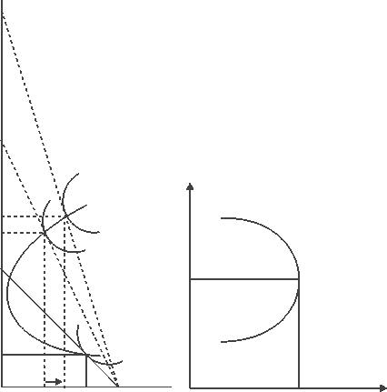
34.2 Derivation of Supply Curve of labour
The supply curve of labour is derived with the help of Indifference curve analysis. Indifference curve shows trade-off between income and leisure (that is, preference between work and leisure)
With increase in wage rate, the total hours of work may increase or decrease depending on the relative strength of income effect and substitution effect.
Since Work is bad, leisure is good; Therefore, Income effect (I.E.) : induces the labour to enjoy more leisure hours, that is, work less
Substitution effect (S.E.) : induces the labour to work for more hours, that is, leisure less.
Maximum hours available in a day (24 hours) OB
It can be used either for:
(i) Work: measured from right to left on X- axis or
(ii) Leisure: measured from origin [left] to the right on X-axis
Note: Income- leisure trade off line AB, A1B---shows combination of time spent on work and leisure
Slope of MA or Income Leisure Tradeoff Line = OM = W1XOA = W1 OA OA
OA = 24 hours
If OM = Rs. 240 W1 = 240 = 10 24
If OM1 = 480; W2 = 480 = 20 24
34.1 : SUPPLY CURVE OF LABOUR
34.2 : BACKWARD BENDING SUPPLY
(i) If entire OB hours is used for leisure : income earned (wages) = 0 (No wages).
(ii) If entire OB hours is used for work : maximum wages (income) earned OA.
(iii) Labour will make a choice between work and leisure. This is at the point where Income Leisure trade line (AB) is tangent to the income leisure trade off curve : (I0) at point E.
He uses OL0 hours for leisure and L0B hours for work, at the wage rate W1 (Fig. 34.1)
If the rm wants the labour to increase his work hours, he will have to give higher wages, Therefore, income – leisure trade off line rotates (swivel) around point B (Reason: 24 hours is xed). New income – leisure trade off line A1B is tangent to the Indifference curve (I1) at point E1
FIG.
FIG.
Para 34.2
Thus, at a higher wage rate W2 (OW2> OW1)
equilibrium point : E1
(iv) Initially since S.E > I.E
hours of work increases to L1B; hours of leisure decreases to OL1, Income earned : OM1
Thus, supply curve has a positive slope (Fig. 34.3)
( v ) If wages increase further to OW 3 (OW3> OW2) I.E>S.E
equilibrium point : E2 hours of work decreases to L2B hours of leisure increases to OL2
Income earned : OM2 (OM2>OM1)
Supply curve has a negative slope. (Fig. 34.4)
By joining points e0, e1, e2, the wage offer curve, that is, the supply curve of labour is derived which is backward bending.
Thus, supply curve of labour shows the relationship between the wage rate and the number of hours worked.
CONCLUSION:
when wage rate increases:
1. initially work hours increase (at low level of wage rate) : SE is stronger than IE
2. later leisure hours increase : (At very high income, level beyond OW2
Works more, leisure less
IE stronger than SE
Work less, leisure more
Thus, increase in wages beyond a certain level, leads to fall in work–hours because labour prefers leisure to work. Therefore, supply curve is backward bending curve.
Non-Economic factors (determinants) of supply of labour:
(a) Labour force: Labour force participation rate in any production activity will depend on some non-economic considerations like job-security, prestige etc. Due to non-economic considerations labour will stick to a particular job and therefore labour becomes immobile between different occupations.
(
b) Size of population: Size of population and age composition determines the supply of labour. The size of population depends on:
(i) population growth rate.
(ii) immigration rate (which is immigration minus migration).
34.3 Market Supply of Labour
Market supply curve of labour is positively sloped. It is not backward bending. Reasons:
(i) Although high wages may induce some people to work less but at the same time new workers will enter the market in the long run.
(ii) If wages are very high unemployed workers who were not willing to work earlier may now undertake training and take up jobs.
(iii) High wages attract young students. They will plan their education in such a manner that they enter the labour force.
(iv) In the long run there is greater occupational and geographical mobility. (Backward bending supply curve is found mostly in the rich nations.)
34.4 Game Theory
Game theory is a mathematical tool for analysing the nature of inter-dependence among the rival rms which was introduced in the works of John von Neumann in the 1920s. Von Neumann, Oskar Morgenstern, and John Nash were the main contributors to the development of game theory.
It helps to understand the role of uncertainty in price and output decisions. Objective of each rm is to maximise pro t or minimise loss, when it is competing with number of competitors. For this purpose, business rms should be able to assess the rival’s actions for which he not only sees competitive situation from his view point but also puts himself in rival’s position to analyse the situation and thus, make an optimal decision.
The game theory provides an insight into the real-world behaviour of the rms (economic agents) in situations when there is con ict of interest. The game arises because the outcome depends not only on the choices made by one player, but also on what other players chose to do at the same time. Thus, game is a situation in which intelligent decisions are necessarily interdependent. To analyse an economic situation using game theory, one must perform two important tasks:
1. To translate the situation into a simple game i.e. simplify the setting as much as possible by retaining only a few essential elements.
2. To “solve” the given game to predict the outcome. To solve a game, an equilibrium concept (such as Nash equilibrium) is applied to the given game by doing the necessary computations.
A game is a conceptual representation of a strategic situation. Even the simplest of games have three essential elements: players, strategies and payoffs. But to properly describe a game in complex situations, additional elements such as the sequence of moves and the information that players have when they move (who knows what when) are also speci ed.
34.5 Basic Terminology
Game: Any set of circumstances where the outcome depends on the actions of two or more players (decision-makers). The players in the game try to maximize their own payoffs.
Players: A strategic decision-maker within the context of the game. These players may be individuals (as in poker games), firms (as in markets with few firms), or entire nations (as in military conflicts).
Pay off: Pay off is the outcome (final returns) of the strategy i.e. whether the player wins or loses at the end of the game. Players are assumed to prefer higher payoffs than lower payoffs. In an oligopoly, firms are the players and their payoffs are the profits in the long run. Each player must choose a strategy.
Strategy: Strategy is the course of action taken by the player in every conceivable situation. Depending on the game being examined, a strategy may be a simple action or a complex plan of action that may be contingent on earlier play in the game.
Information set: The information available at a given point in the game. Usually, this term is applied when the game has a sequential component.
Equilibrium: The point in a game where both players have made their decisions and an outcome is reached. Equilibrium occurs when each player chooses the best strategy, given the strategies followed by other players. This is called Nash equilibrium. Nobody wants to change their strategy because while calculating the best strategy each player has already taken into account the strategy followed by their rival firms.
Sometimes a player’s best strategy is independent of the strategy chosen by others. It is called dominant strategy.
34.6 Types of Game Theory
34.6-1 Cooperative vs. Non-Cooperative Games
Cooperative game theory is the most popular kind of game theory that examines how cooperative groups, or coalitions, behave when just the payoffs are known. Instead of being a game between two players, it is a coalition game that explores the formation of groups and how they distribute payoffs among themselves. Non-cooperative game theory focuses on the interactions between rational economic agents who aim to achieve their individual objectives. The most prevalent
form of non-cooperative game is the strategic game, which outlines the possible strategies and the outcomes arising from different combinations of choices. A simple real-world example of a non-cooperative game is rock-paper-scissors.
34.6-2
Zero-Sum vs. Non-Zero-Sum Games
A zero-sum game is one in which several participants directly compete with one another to achieve the same goal. This implies that for every winner, there is a corresponding loser meaning the total bene t gained is equal to the total bene t lost. Many sporting events exemplify zero-sum games, where one team wins, and the other loses.
A non-zero-sum game is a situation where all participants can simultaneously gain or lose. For example, in business partnerships that are mutually bene cial, both parties work together to create value rather than competing against each other. This collaborative approach allows both entities to bene t.
34.6-3
Simultaneous Move vs. Sequential Move Games
In situations involving simultaneous moves, both the player and his competitors make decisions at the same time. For instance, as one company develops its marketing, product, and operational strategies, its rivals are simultaneously preparing similar strategies.
In situations involving sequential moves, decision-making steps are deliberately staggered to allow one party to observe the other party’s moves before making their own. This approach is commonly seen in negotiations: one party presents their demands, and then the other party is given a speci c period to respond and state their own demands.
34.6-4
One Shot vs. Repeated Games
Game theory can be a single, self-contained event where the competition starts, unfolds, and concludes, without the possibility of replaying it. This is particularly true for equity traders, who must carefully select their entry and exit points, as their decisions are often irreversible.
On the other hand, repeated games persist inde nitely and seem to go on forever. These games typically involve the same participants each time, with each party aware of past events. For instance, think about competing companies setting their prices. When one company changes its price, the other may respond similarly. This ongoing cycle of competition continues through various product cycles or sales seasons.
34.7 Rule of Game
Each decision maker is a player. Each game is played by a set of rules which speci es 4 things : (1) Who is playing ?
(2) What are they playing? i.e. actions/choice/strategies available with each player.
(3) When each player plays ?
(4) Probability of gain or loss from the choice made.
Two ways to represent the rules of the game:
1. Normal form - Strategic form.
2. Extensive form - presented in pictorial form like game tree.
Every player knows the rules of the game.
e.g. of strategic form game :
(i) Prisoners Dilemma.
(ii) Battle of sexes.
34.8 Prisoners’ Dilemma
The Prisoners’ Dilemma, introduced by A. W. Tucker in the 1940s, is one of the most famous games studied in game theory.
Situation
There are two suspects (player 1 and player 2) who have been arrested for a crime. Due to lack of evidence each suspect is kept in separate cell (prison) and interrogated separately.
During interrogation police tells each:
(i) If you confess but your companion doesn’t confess, you will get reduced (one-year) sentence, whereas your companion will get four years.
(ii) If you both confess, you will each get a three-year sentence.
(iii) Each suspect also knows that if neither of them confesses, then due to lack of evidence, both will be sentenced for two-years.
Outcome
Case I
Extensive Form
The game tree, also called the extensive form, is shown in Figure 34.5. The action proceeds from left to right. Each node (shown as a dot on the tree) represents a decision point for the player indicated there.
The first move in this game belongs to player 1 (suspect1); he must choose whether to confess or be silent.
Then player 2 makes his decision.
The dotted oval drawn around the nodes at which player 2 moves indicates that the two nodes are in the same information set, that is, player 2 does not know what player 1 has chosen when 2 moves.
We put the two nodes in the same information set because the police approaches each suspect separately and does not reveal what the other has chosen.
Note: Payoffs are given at the end of the tree (listed at the right). The convention is for player 1’s payoff to be listed rst, then player 2’s.
Case II
Table 34.1 Normal form for Prisoners’ Dilemma
Although the extensive form of the structure of the game is visually appealing, sometimes it is more convenient to represent games in matrix form, called the normal form of the game as shown in Table 34.1.
Table 34.1
Player (Suspect) 2 Player (Suspect)
Player 1 is the row player
Player 2 is the column player.
Each entry in the matrix lists the payoffs rst for player 1 and then for 2.
Table 34.2
Underlining procedure for Prisoners’ Dilemma
Player (Suspect) 2 Player (Suspect)
FIG. 34.5: EXTENSIVE FORM
Para 34.9
A quick way to nd the Nash equilibria of a game is to underline best-response payoffs in the matrix. The underlining procedure is demonstrated for the Prisoners` Dilemma in Table 34.2
Underline the payoffs corresponding to player 1’s best responses.
Player 1’s best response is to confess if player 2 confesses, so we underline p1 = 1 in the upper left box, and to confess if player 2 is silent, so we underline p1 = 3 in the upper right box.
Next, underline the payoffs corresponding to player 2’s best responses.
Player 2’s best response is to confess if player 1 confesses, so we underline p2 = 1 in the upper left box, and to confess if player 1 is silent, so we underline p2 = 3 in the lower left box.
After underlining the best-response payoffs, we search for boxes where every player’s payoff is underlined. These boxes represent Nash equilibria.
In Table 34.2 only the upper left box shows both payoffs underlined, confirming that (confess, confess) the only Nash equilibrium, with none of the other outcomes meeting this criterion.
34.9 Strategy Adopted in Prisoners’ Dilemma
What will be the outcome in the Prisoners Dilemma?
Prisoners are faced with a dilemma: confess or not to confess.
The table 34.1 initially suggests that one might expect both to remain silent. This would grant both the players (suspects) a combined total of four years of freedom as compared to any other outcome
However, this may not be the best prediction in the game.
Imagine player 1’s position for a moment. He does not know what player 2 will do.
Possibilities:
1. Suppose player 2 chose to confess. By confessing, he would get one year of freedom as compared to none if he remained silent, so Confessing is better for him.
2. Suppose player 2 chose to remain silent. Confessing is still better for him than remaining silent since he will get three rather than two years of freedom.
Since the players are symmetric in the Prisoner’s Dilemma, the optimal prediction is that both players (suspects) will choose to confess, resulting in the outcome (confess, confess).