Power System Analysis and Design SI Edition 6th Edition Glover Solutions Manual Visit to Download in Full: https://testbankdeal.com/download/power-system-analysis-a nd-design-si-edition-6th-edition-glover-solutions-manual/
Chapter 2 Fundamentals
1 © 2017 Cengage Learning®. May not be scanned, copied or duplicated, or posted to a publicly accessible website, in whole or in part.
ANSWERSTOMULTIPLE-CHOICETYPEQUESTIONS 2.1 b 2.2 a 2.3 c 2.4 a 2.5 b 2.6 c 2.7 a 2.8 c 2.9 a 2.10 c 2.11 a 2.12 b 2.13 b 2.14 c 2.15 a 2.16 b 2.17 A. a B. b C. a 2.18 c 2.19 a 2.20 A. c B. a C. b 2.21 a 2.22 a 2.23 b 2.24 a 2.25 a 2.26 b 2.27 a 2.28 b 2.29 a 2.30 (i) c (ii) b (iii)a (iv)d 2.31 a 2.32 a Power System Analysis and Design SI Edition 6th Edition Glover Solutions Manual Visit TestBankDeal.com to get complete for all chapters
2.1 (a) [ ] 1 6306cos30sin305.20 3 Ajj =∠°=°+°=+
(b) 1 128.66 2 5 451625tan6.40128.666.40 4 j Aj e ° =−+=+∠=∠°=
(c) ( ) ( ) 3 5.203451.2088.0181.50Ajjj =++−+=+=∠°
(d) ( )( ) 4 6306.40128.6638.414158.65835.7813.98 A j =∠°∠°=∠°=−+
(e) ( ) ( ) 158.66 5 630/6.40128.660.94158.660.94 j A e ° =∠°∠−°=∠°=
2.2 (a) 50030433.01250Ij =∠−°=−
(b) ( ) ( ) ( ) ()4sin304cos30904cos60 itttt ωωω =+°=+°−°=−°
( ) 4602.83601.422.45Ij =∠−°=∠−°=−
(c) ( ) ()() 5/2154603.420.9223.46 Ijj =∠−°+∠−°=−+−
5.424.386.96438.94 j =−=∠−°
2.3 (a) maxmax400V;100AVI==
(b) 4002282.84V;100270.71AVI ====
(c) 282.8430V;70.7180AVI=∠°=∠−°
2017
2 ©
publicly
Cengage Learning®. May not be scanned, copied or duplicated, or posted to a
accessible website, in whole or in part.
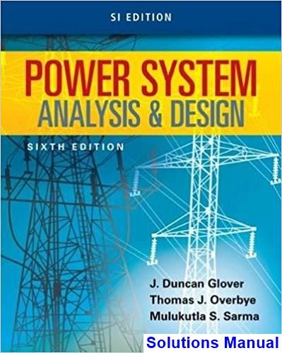
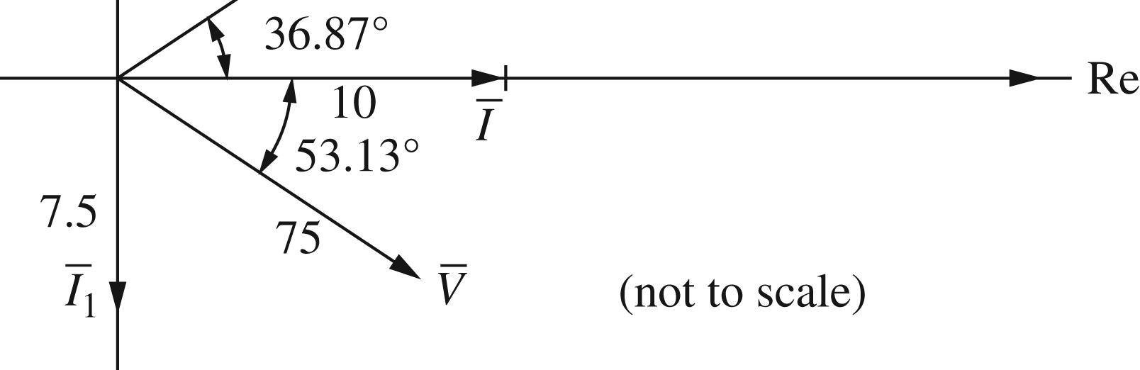
2.4 (a) ()()() 1 21 2 6690 100107.590A 8668 1007.390107.512.536.87A 612.536.876907553.13V j I jj IIIj VIj −∠−° =∠°==∠−° +− =−=∠°−∠−°=+=∠° =−=∠°∠−°=∠−° (b) 2.5 (a) ( ) ( ) ()2772cos30391.7cos30V ttt υωω=+°=+° (b) () /2013.8530A ()19.58cos30A IV itt ω ==∠° =+° (c) ( )( ) ()() ()() 3 26010103.77190 277303.7719073.4660A ()73.462cos60103.9cos60A ZjLj IVZ ittt ωπ ωω ==×=∠°Ω ==∠°∠°=∠−° =−°=−°
(d)
25 27730259011.08120A
()11.082cos12015.67cos120A
ittt ωω
2.6 (a) ( ) 7521553.0315 V =∠−°=∠−° ; ωdoes not appear in the answer.
(b) ( ) ()502cos10 tt υω=+° ; with ω= 377, ( ) ()70.71cos37710 tt υ =+°
(c);;AABBCAB αβ =∠=∠=+
=+=
()()()2Re jt ctatbtCe ω
Theresultant has the same frequency ω.
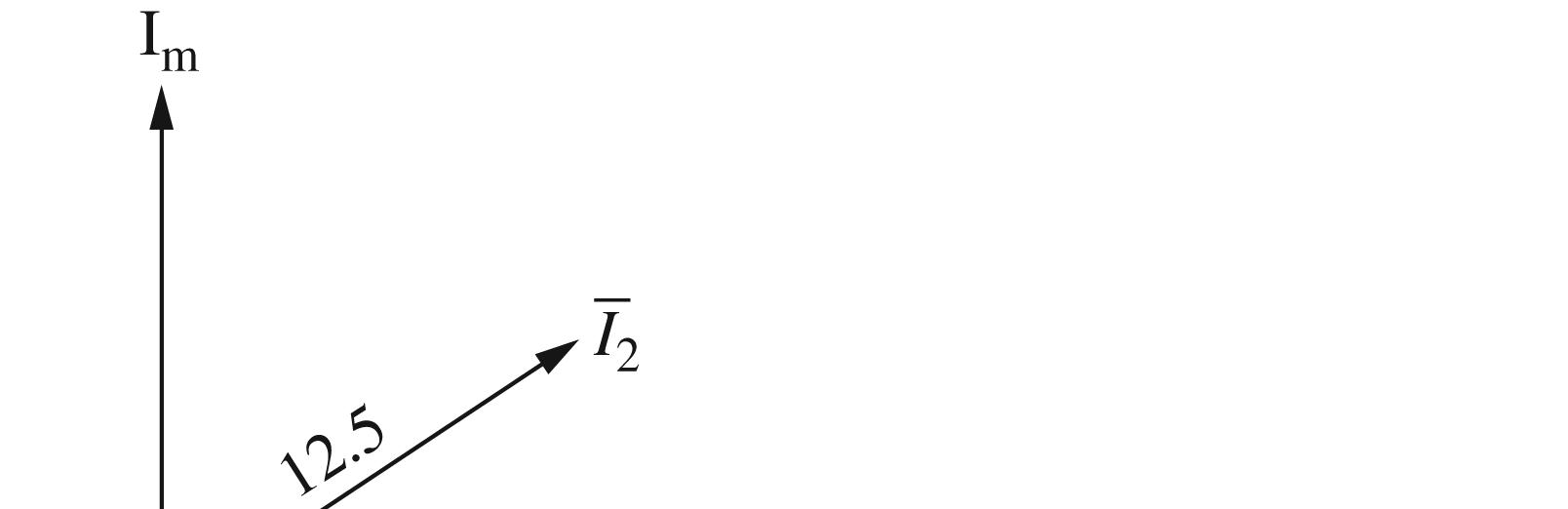
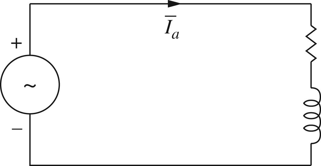
2.7 (a) Thecircuit diagramis shown below:
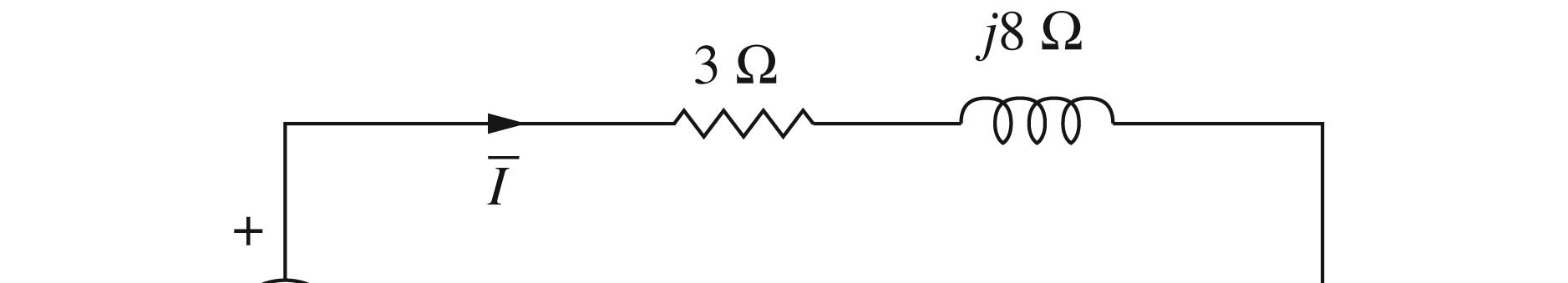
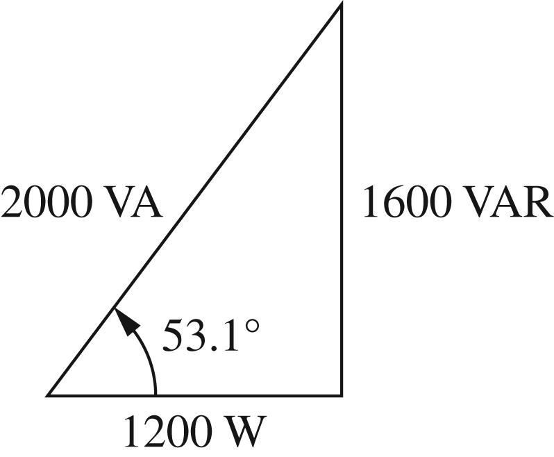
(b) 38434553.1Zjjj=+−=+=∠°Ω
(c) ( ) ( ) 1000553.12053.1A I =∠°∠°=∠−°
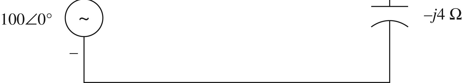
Thecurrent lags thesourcevoltage by53.1° Power Factorcos53.10.6 Lagging =°=
© 2017 Cengage Learning®. May not be scanned,
3
copied
duplicated, or posted to a publicly accessible
whole or
or
website, in
in part.
()() ()()
Zj IVZ
=−Ω ==∠°∠−°=∠° =+°=+°
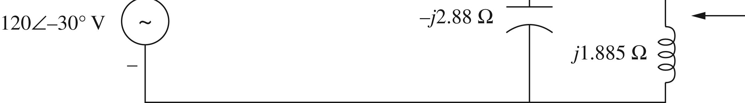
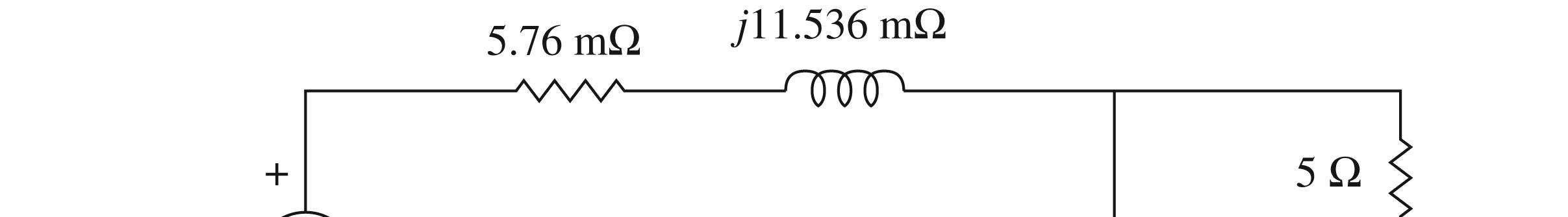
2.8 ( )( ) ()() ()() 6 3 6 37730.61011.536m 3775101.885 1 2.88 37792110 1202 30V 2 LT LL C Zjj Zjj Zjj V =×=Ω =×=Ω =−=−Ω × =∠−°
Thecircuit transformed tophasor domain is shownbelow:
4 © 2017 Cengage Learning®. May not be scanned, copied or duplicated, or posted to a publicly accessible website, in whole or in part.
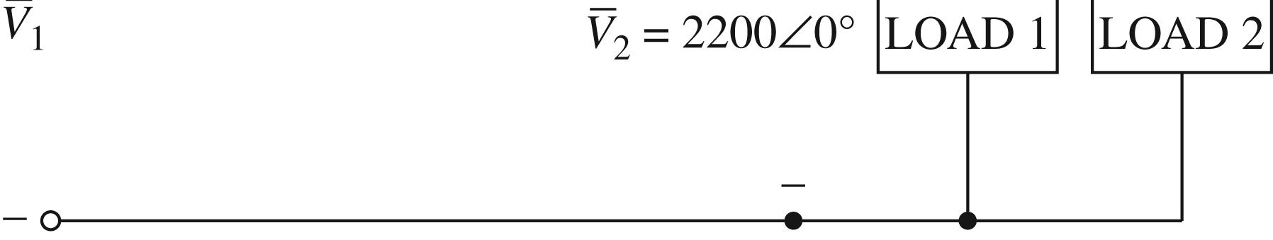
2.9 ( )( ) ()() :12006000.10.5 12006000.10.5 114.130.0117.914.7V LOAD LOAD KVLjV Vj j ∠°=∠°++ ∴=∠°−∠°+ =−=∠−°← 2.10 (a) ( ) ( ) ()()() () 4 ()()()400cos30100cos80 1 400100cos110cos250 2 6840.4210cos250W pttittt t t υωω ω ω ==+°−° =°+−° =−+×−° (b) ( ) ( )( ) ( ) cos282.8470.71 cos3080 6840WAbsorbed +6840 WDelivered PVI δβ =−=°+° =− = (c) ( ) ( )( ) sin282.8470.71sin110 18.79 kVAR Absorbed QVI δβ =−=° = (d)Thephasor current ( ) 70.718018070.71100 I −=∠−°+°=∠° A leaves thepositive terminal of the generator. Thegenerator power factor is then ( ) cos301000.3420 °−°= leading 2.11 (a) ( ) () () () () 2 4 33 ()()()391.719.58cos30 1 0.7669101cos260 2 3.834103.83410cos260W cos27713.85cos03.836kW sin0VAR pttitt t t PVI QVI υω ω ω δβ δβ ==×+° =×++° =×+×+° =−=×°= =−= ( ) ( ) SourcePower Factorcoscos30301.0 δβ =−=°−°= (b) ( ) ( ) () () ()() υωω ω ω δβ ==×+°−° =×°+−° =×−° =−=×°+°= 4 4 ()()()391.7103.9cos30cos60 1 4.0710cos90cos230 2 2.03510cos230W cos27773.46cos30600W pttittt t t PVI ( ) () δβ δβ =−=×°= =−= sin27773.46sin9020.35kVAR cos0 Lagging QVI pf
5 © 2017 Cengage Learning®. May not be scanned, copied or duplicated, or posted to a publicly accessible website, in whole or in part. (c) ( ) ( ) ()()()391.715.67cos30cos120 pttittt υωω ==×+°+° ()()() ()() ()() ()() 3 3 1 6.13810cos90cos21503.06910cos2150W 2 cos27711.08cos301200W sin27711.08sin90 3.069kVAR Absorbed3.069kVAR Delivered coscos900Leading tt PVI QVI pf ωω δβ δβ δβ =×−°++°=×+° =−=×°−°= =−=×−° =−=+ =−=−°= 2.12 (a) ( )( ) ()359.3cos35.93cos 64556455cos2W R pttt t ωω ω = =+ (b) ( ) ( ) () ()359.3cos14.37cos90 2582cos2cot90 2582sin2W x pttt t ωω ω =+° =+° =− (c) ( )2 2 359.32106455W Absorbed PVR=== (d) ( )2 2 359.32252582VARSDelivered QVX=== (e) ( ) ( ) ( ) ()() 11 tan/tan2582645521.8 Powerfactorcoscos21.80.9285 Leading QP βδ δβ −===° =−=°= 2.13 ()() () 102526.9368.2 ()359.3/26.93cos68.2 13.34cos68.2A c ZRjxj itt t ω ω =−=−=∠−°Ω =+° =+° (a) ( ) ( ) () ()13.34cos68.2133.4cos68.2 889.8889.8cos268.2W R pttt t ωω ω =+°+° =++° (b) ( ) ( ) () ()13.34cos68.2333.5cos68.290 2224sin268.2W x pttt t ωω ω =+°+°−° =+° (c) ( )2 2 13.34210889.8W PIR=== (d) ( )2 2 13.342252224VARS QIX=== (e) ( ) 11 costan/costan(2224/889.8) 0.3714 Leading pfQP == =
(b) ( ) ( ) cos62cos4508.49MWDelivered PVI δβ
(d) ( ) ( ) coscos4500.707
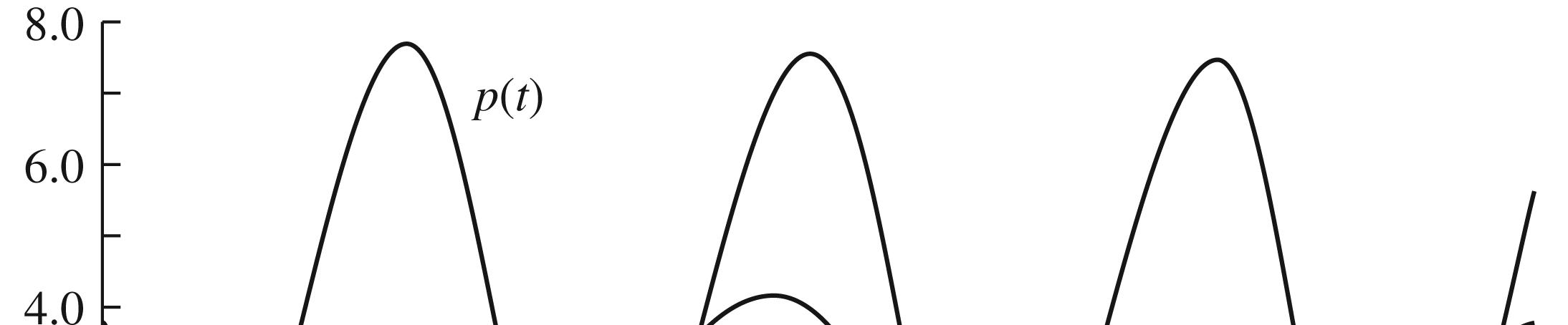
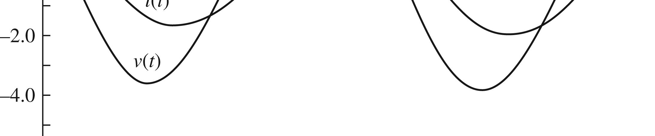
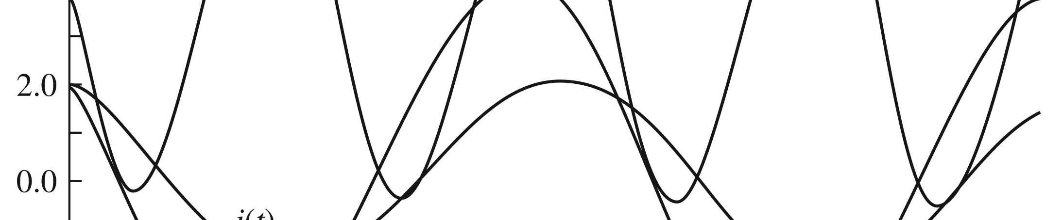
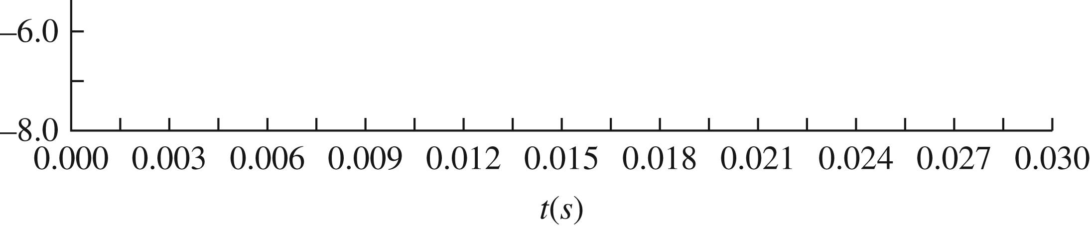
(b) υ(t), i(t), and p(t
(c) The instantaneous power has an average value of 3.46 W, and the frequency is twice that of the voltage or current.
6 © 2017 Cengage Learning®. May not be scanned, copied or duplicated, or posted to a publicly accessible website, in whole or in part. 2.14 (a) 20kA I =∠° ( )( ) () () ()() () 34520645kV ()62cos45kV ()()()62cos4522cos 1 24cos45cos245 2 8.4912cos245MW VZI tt pttittt t t υω υωω ω ω ==∠−°∠°=∠−° =−° ==−° =−°+−° =+−°
sin62sin450
QVI δβ =−=×−°−° =−=+
=−=×−°−°= (c) ( ) ( )
8.49MVARDelivered8.49MVARAbsorbed
pf δβ =−=−°−°= 2.15 (a) ( ) () 4260230230A I =∠°∠°=∠° ( ) () () ()2cos30A with 377rad/s ()()()4cos30cos290 3.464cos290W itt pttitt t ωω υω ω =+°= ==°++° =++°
Leading
)
plotted
are
below.
2.16
(a) 101200.041015.118.156.4Zjj π =+×=+=∠°Ω cos56.40.553 Lagging pf =°=
(b) 1200V V =∠°
The current supplied by the source is ( ) ( ) 120018.156.46.6356.4A I =∠°∠°=∠−°
The real power absorbed by the load is given by 1206.63cos56.4440W P =××°=
which can be checked by ()2 2 6.6310440W IR ==
The reactive power absorbed by the load is 1206.63sin36.4663VAR Q =××°=
(c) ()2 2 Peak Magnetic Energy0.046.631.76J WLI ==== 3771.76663VAR is satisfied. QW ω ==×=
**2 SVIZIIZIjLI
(b) ()()2sin di tLLIt
Average real power supplied to the inductor0 P =←
Instantaneous power supplied (to sustain the changing energy in the magnetic field) has a maximum value of Q. ←
(b)Choosing
7 ©
Cengage Learning®. May not be scanned, copied or duplicated, or posted to a publicly accessible website, in whole or in part.
2017
2
2
QSLI ω ==←
2.17 (a)
ω ====
Im[]
dt
==−+ ( ) ( ) () () 2 2 ()()()2sincos sin2 sin2 pttitLItt LIt Qt υωωθωθ ωωθ ωθ =⋅=−++ =−+← =−+←
υωωθ
2.18 (a)
===+ 22 cos;sin PjQ PZIZQZIZ =+ ∴=∠=∠←
**22 ReIm SVIZIIZIjZI
( ) () [ ] 2 2 2 ()()()coscos coscos2 coscos2cossin2sin (1cos2)sin2 pttitZItZt ZIZtZ ZIZtZtZ PtQt υωω ω ωω ωω ∴=⋅=+∠⋅ =∠++∠ =∠+∠−∠ =+−←
()2cos, itIt ω = Then ( ) ()2cos tZItZυω=+∠
8 © 2017 Cengage Learning®. May not be scanned, copied or duplicated, or posted to a publicly accessible website, in whole or in part. (c) 1 ZRjL jC ω ω =++ Frompart(a), 2 PRI = and LCQQQ =+ where 2 L QLI ω= and 2 1 C QI Cω =− whicharethereactivepowersinto L and C,respectively. Thus ( ) ()1cos2sin2sin2 LC ptPtQtQt ωωω =+−−← () 2 If 1,0 Then ()1cos2 LC LCQQQ ptPt ω ω =+== ← =+ 2.19 (a) * * 1505 105037560 22 187.5324.8 SVI j ==∠°∠−°=∠° =+ Re187.5WAbsorbed Im324.8VARSAbsorbed PS QS == == (b) ( ) cos600.5 Lagging pf =°= (c) 1 tan187.5tancos0.990.81VARS 324.890.81234VARS SS CLS QPQ QQQ === =−=−= 2.20 () 1 11 1 11 0.05300.04330.025S 2030 Y jGjB Z ===∠−°=−=− ∠° () () () () () 2 22 2 2 2 11 2 2 11 2 2 22 2 2 22 11 0.04600.020.03464S 2560 1000.0433433WAbsorbed 1000.025250VARSAbsorbed 1000.02200WAbsorbed 1000.03464346.4VARSAbsorbed Y jGjB Z PVG QVB PVG QVB ===∠−°=−=+ ∠° === === === ===
9 © 2017 Cengage Learning®. May not be scanned, copied or duplicated, or posted to a publicly accessible website, in whole or in part. 2.21 (a) 1 1 cos0.653.13 tan500tan53.13666.7 kVAR cos0.925.84 L LL S QP φ φ φ ==° ==°= ==° tan500tan25.84242.2kVAR 666.7242.2424.5kVAR 424.5kVA SS CLS CC QP QQQ SQ φ ==°= =−=−= == (b)The 375 synchronous motor absorbs416.7kW 0.9 m P == and 0kVAR mQ = PS = P + Pm = 500 + 416.7 = 916.7 kW Source ( ) 1 PFcostan666.7916.70.809 Lagging == 2.22 (a) () () 1 1 111 0.1651.34 456.451.34 0.10.12S Y Zj j ====∠−° +∠° =− () () () () 2 2 2 12 12 2 2 11 2 2 22 11 0.1S 10 1000 70.71 V 0.10.1 70.710.1500W 70.710.1500W Y Z P PVGGV GG PVG PVG === =+⇒=== ++ === === (b) ( ) 12 0.10.120.10.20.12 0.23330.96S eq YYYjj =+=−+=− =∠−° ( ) 70.710.23316.48A SeqIVY===
2.26
The problem is modeled as shown in figure below:
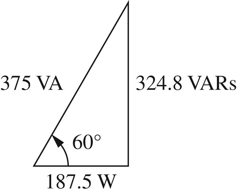
Power triangle for the load:
10 © 2017 Cengage Learning®. May not be scanned, copied or duplicated, or posted to a publicly accessible website, in whole or in part. 2.23 ( )( ) * 12001530180030 1558.85900 Re1558.85WDelivered Im900VARSDelivered900VARSAbsorbed SVI j PS QS ==∠°∠−°=∠−° =− == ==−=+ 2.24 1 1112100;10cos0.994.359SPjQjSj =+=+=∠=+ 1 3 123 7.5 cos0.959.28818.198.8242.899 0.850.95 27.821.46027.863.00 Re()27.82kW Im()1.460kVAR 27.86kVA S SS SS SS S j SSSSj PS QS SS =∠−=∠−°=− × =++=+=∠° == == == 2.25 **22 **22 **22 (20)312000 ()8(20)03200 ()4(20)01600 RR LLLL CCCC SVIRIIIRj SVIjXIIjXIjj SVIjIXIjXIjj =====+ =====+ ==−=−=−=− Complex power absorbed by the total load 200053.1 LOADRLC SSSS=++=∠°
Triangle: Complex power
()()* * 10002053.1200053.1 SOURCE SVI==∠°∠−°=∠°
Power
delivered by the source is
The complex power delivered by the source is equal to the total complex power absorbed by the load.
1 120kW 0.85Lagging cos0.8531.79 L L L P pf θ = = ==°
(a)
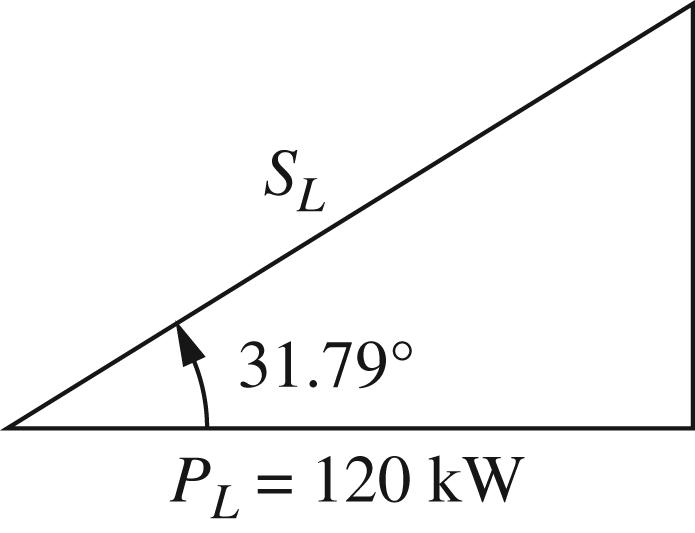
11 © 2017 Cengage Learning®. May not be scanned, copied or duplicated, or posted to a publicly accessible website, in whole or in part. 141.1831.79kVA /141,180/480294.13A LLL L SPjQ ISV =+=∠° === ( ) tan31.79 74.364kVAR LL QP=° =
power loss
zero. Reactive power loss in the line is ()2 2 294.131 LINELINEQIX== 86.512kVAR = ( ) 12074.36486.512200.753.28kVA SSS SPjQj ∴=+=++=∠°
input
SS VSI== The power
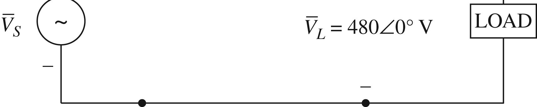
cos53.280.6 Lagging °= (b)Applying KVL, ( ) 48001.0294.1331.79 S Vj=∠°+∠−° () 635250682.421.5V(rms) ()cos21.531.790.6 Lagging S j pf =+=∠° =°+°=
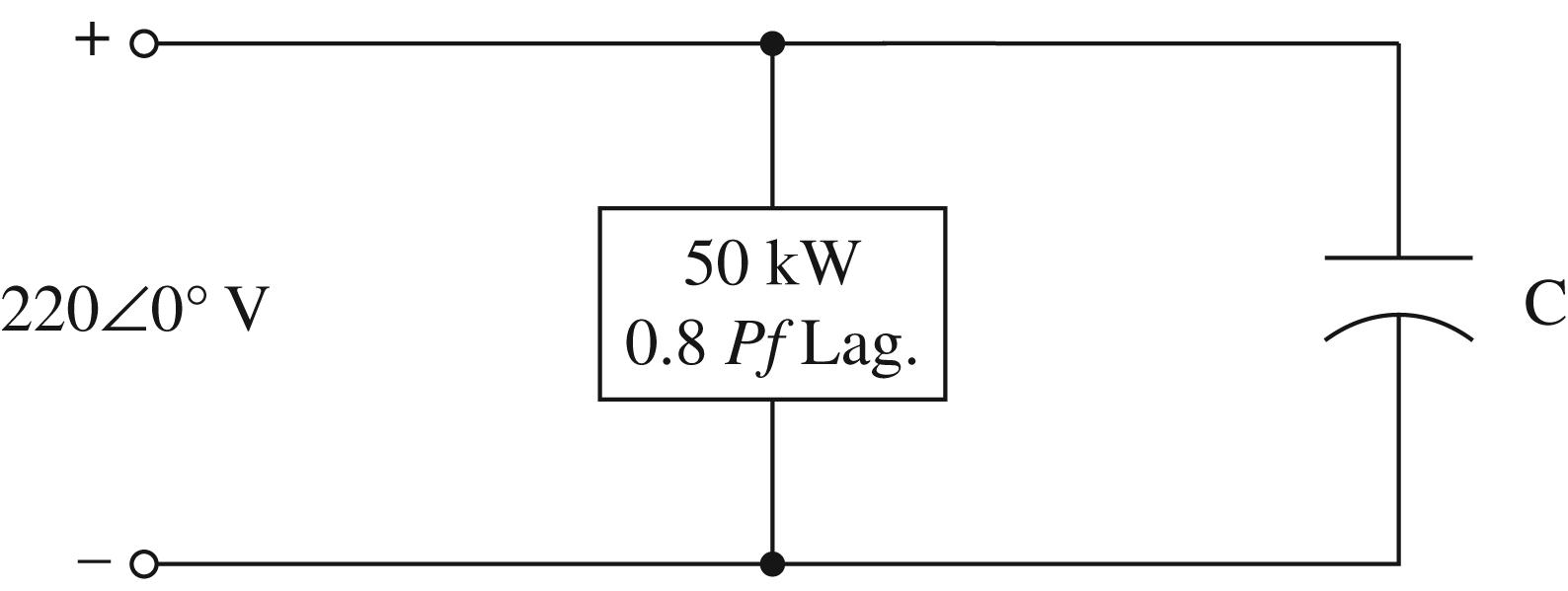
( ) 1 50kW;cos0.836.87;36.87;tan 37.5kVAR old OLDoldoldold P QP θθ==°=°= = 50,00037,500 old Sj ∴=+ ( ) 1 cos0.9518.19;50,00050,000tan18.19 50,00016,430 new new Sj j θ ==°=+° =+ Hence 21,070VA capnewold SSSj =−=− ()()2 21,070 1155F 377220 C µ ∴==←
Real
in the line is
The
voltage is given by /682.4V(rms)
factor at the input is
2.27 The circuit diagram is shown below:
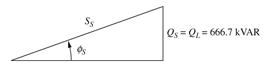
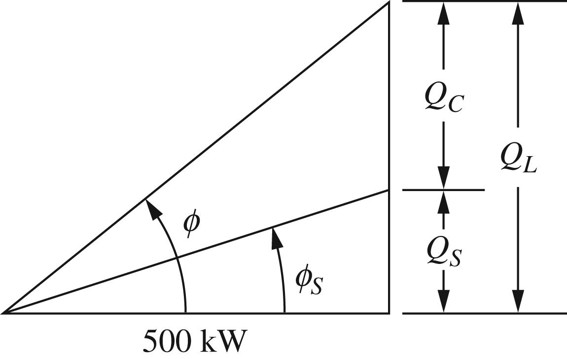
12 © 2017 Cengage Learning®. May not be scanned, copied or duplicated, or posted to a publicly accessible website, in whole or in part. 2.28 () () () 1 1 2 3 123 156.667 30.963sincos0.962.880.84 150 32.885.827kVA TOTAL Sj Sjj Sj SSSSj =+ =−=− =+ =++=+ (i) Let Z be the impedance of a series combination of R and X Since * 2 * * VV SVIV ZZ === , it follows that ( ) () () 2 2 * 3 240 (1.6980.301) 32.885.82710 1.6980.301 V Z j Sj Zj ===−Ω + ∴=+Ω← (ii)Let Z be the impedance of a parallel combination of R and X Then () () () () () 2 3 2 3 240 1.7518 32.8810 240 9.885 5.82710 1.75189.885 R X Zj ==Ω ==Ω ∴=Ω← 2.29 Sincecomplex powers satisfyKCL ateachbus,itfollows that ( ) ( ) ( ) 13 * 3113 11110.40.20.41.8 0.41.8 Sjjjj SSj =+−−−+=−+← =−=+← Similarly, ( ) ( ) ( ) 23 0.50.5110.40.20.10.7 Sjjjj =+−+−−+=−−← * 3223 0.10.7SSj=−=−← At Bus 3, ( ) ( ) 33132 0.41.80.10.70.51.1 G SSSjjj =+=++−=+← 2.30 (a) For load 1: 1 1 cos(0.28)73.74 Lagging θ ==° 1 2 3 12573.7435120 1040 150 Sj Sj Sj =∠°=+ =− =+ () 123 608010053.13kVA 60kW;80kVAR;kVA100kVA. Supplycos53.130.6 Lagging TOTAL TOTALTOTALTOTALTOTAL SSSSjPjQ PQS pf =++=+=∠°=+ ∴====← =°=← (b) *3 * 1001053.13 10053.13A 10000 TOTAL S I V ×∠−° ===∠−° ∠° At thenew pf of 0.8 lagging, PTOTAL of 60kW resultsinthe newreactive power Q′ , suchthat
13 © 2017 Cengage Learning®. May not be scanned, copied or duplicated, or posted to a publicly accessible website, in whole or in part. ( ) 1 cos0.836.87 θ′ ==° and ( ) 60tan36.8745kVAR Q′ =°= ∴Therequiredcapacitor’s kVARis 804535kVAR CQ =−=← It followsthen ( )2 2 * 1000 28.57 35000 C C V Xj Sj ===−Ω and ()() 610 92.85F 26028.57 C µ π ==← Thenewcurrentis * * 60,00045,000 6045 10000 Sj Ij V ′ ′ ===− ∠° 7536.87A=∠−° Thesupplycurrent, inmagnitude,is reduced from100Ato 75A ← 2.31 (a) 112212 12 129090 90 VVVV I XXX δδ δδ ∠−∠ ==∠−°−∠−° ∠° Complex power 12 * 121121112 2 112 12 9090 9090 VV SVIV XX VVV XX δδδ δδ ==∠∠°−−∠°− =∠°−∠°+− ∴ The realandreactive power atthesendingend are () () 2 112 12 12 12 12 cos90cos90 sin VVV P XX VV X δδ δδ =°−°+− =−← () () 2 112 12 12 1 1212 sin90sin90 cos VVV Q XX V VV X δδ δδ =°−°+− =−−← Note:If 1V leads 2V , 12 δδδ =− ispositiveandtherealpowerflowsfromnode1to node2.If 1V Lags 2V , δ isnegativeandpowerflowsfromnode2tonode1. (b)Maximumpowertransferoccurswhen 12 90 δδδ=°=−← 12 MAX VV P X =←
2.32 4Mvarminimizestherealpowerlinelosses,while4.5MvarminimizestheMVApower flowintothefeeder.
14 © 2017 Cengage Learning®. May not be scanned, copied or duplicated, or posted to a publicly accessible website, in whole or in part. 2.33 Qcap MWLosses MvarLosses 0 0.42 0.84 0.5 0.4 0.8 1 0.383 0.766 1.5 0.369 0.738 2 0.357 0.714 2.5 0.348 0.696 3 0.341 0.682 3.5 0.337 0.675 4 0.336 0.672 4.5 0.337 0.675 5 0.341 0.682 5.5 0.348 0.696 6 0.357 0.714 6.5 0.369 0.738 7 0.383 0.766 7.5 0.4 0.801 8 0.42 0.84 8.5 0.442 0.885 9 0.467 0.934 9.5 0.495 0.99 10 0.525 1.05 2.34 7.5Mvars 2.35
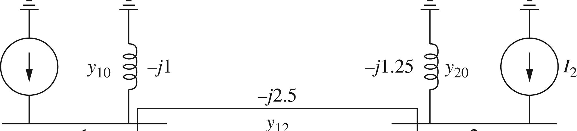
2.36 Note that there are two buses plus the reference bus and one line for this problem. After converting the voltage sources in Fig. 2.29 to current sources, the equivalent source impedances are:
The rest is left as an exercise to the student.
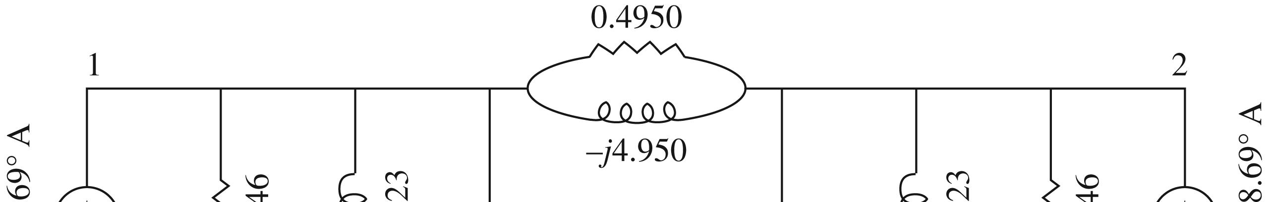
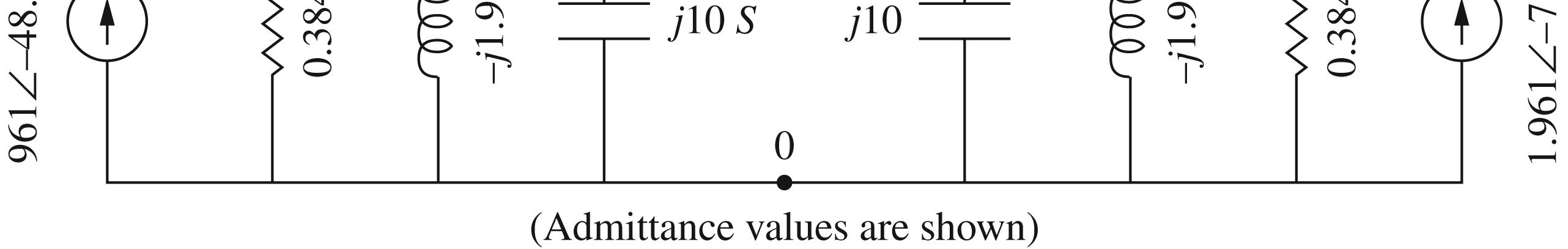
2.37 After converting impedance values in Figure 2.30 to admittance values, the bus admittance matrix is:
15 © 2017 Cengage Learning®. May not be scanned, copied or duplicated, or posted to a publicly accessible website, in whole or in part. ( ) ( ) ( ) ()()() 10 20 .3846.4950101.9234.950.49504.950 .49504.950.3846.4950101.9234.95 1.96148.69 1.96178.69 j j V jj V ++−−−− −−++−− ∠−° = ∠−° 10 20 0.87963.1270.49504.950 1.96148.69 0.49504.9500.87963.127 1.96178.69 jj V jj V +−+ ∠−° = −+−+ ∠−°
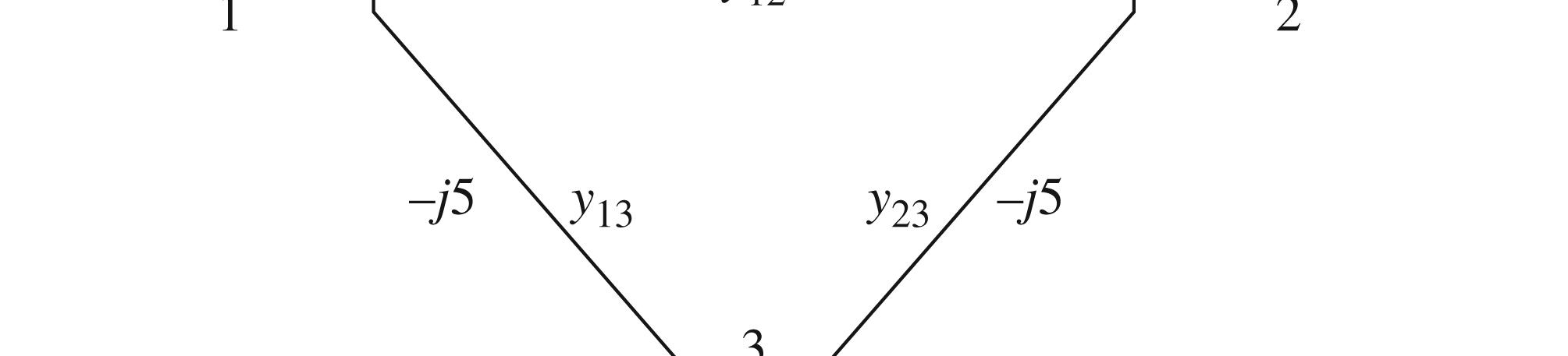
()() ( )( ) ()() 12 0.10.50.1 0.10.50.1 0.10.50.1 0.509978.690.190 0.123787.27 0.412375.96 0.0058820.1235 // SS jj ZZjj jj j +− ==+−= +− ∠°∠−° ==∠−° ∠° =−Ω
1100 11111 1111 23434 11111 011 33424 11111 0 44443 bus jj Y jjjjj jjj −+++−−−− = −−−++− −−+− Writing nodal equations by inspection: () () () () () () 10 20 30 40 10 1010 2.08310.25 10.333310 0.333310.25 00.33330.250 0.250.250.08333 00.25230 V j j V jj j V j j V ∠° −−+ = −+− −∠°
2.38 The admittance diagram for the system is shown below:

16 © 2017 Cengage Learning®. May not be scanned, copied or duplicated, or posted to a publicly accessible website, in whole or in part.
11121314 21222324 31323334 41424344 8.52.55.00 2.58.755.00 5.05.022.512.5 0012.512.5 BUS YYYY YYYY YjS YYYY YYYY − == where 111012132220122323132334 ;; YyyyYyyyYyyy =++=++=++ 4434122112133113233223 ;;; YyYYyYYyYYy ===−==−==− and 344334 YYy ==− 2.39 (a) 11 22 33 44 0 0 0 0 cdf f d c bde d be b cabc e f efg YYYY Y VI Y YYYYYYVI Y VI YYYY YYYYYVI ++− = ++ = = −++ ++ (b) 1 2 3 4 14.5842.50 817450 448.80190 2.5508.30.62135 V V j V V − = −∠−° −∠−° 11 ; BUSBUSBUSBUS YVIYYVYI ==
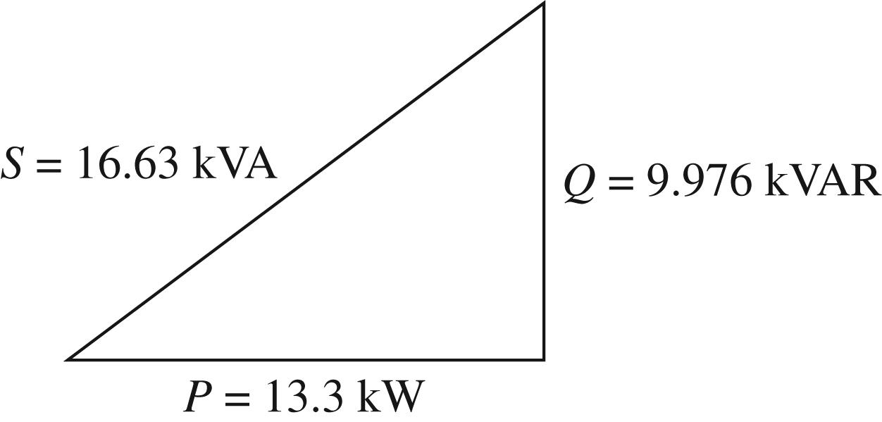
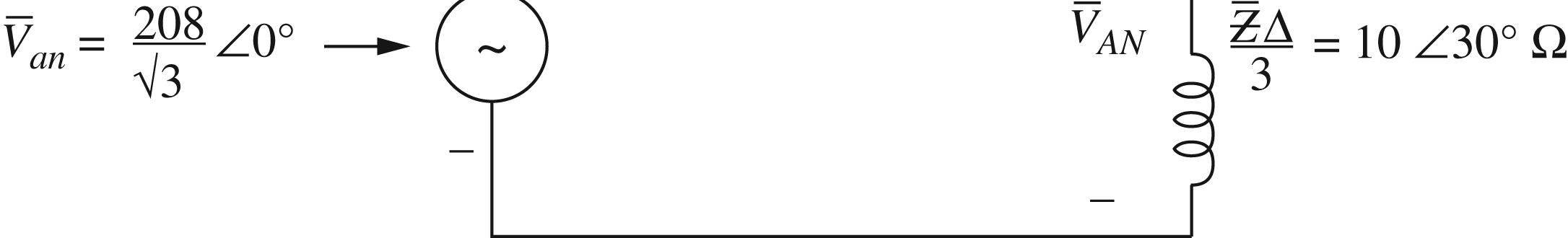
17 © 2017 Cengage Learning®. May not be scanned, copied or duplicated, or posted to a publicly accessible website, in whole or in part. where 1 0.71870.66880.63070.6194 0.66880.70450.62420.6258 0.63070.70450.68400.5660 0.61940.62580.56600.6840 BUSBUS YZj == Ω 1 BUS VYI = where 1 2 3 4 V V V V V = and 0 0 190 0.62135 I = ∠−° ∠−° Then solve for 1V , 2V , 3V , and 4V . 2.40 (a) 240 0138.560V 3 ANV =∠°=∠° (AssumedasReference) () 24030V;24090V;1590A 138.560 9.249009.24 1590 ABBCA AN Y A VVI V Z j I =∠°=∠−°=∠−° ∠° ===∠°=+Ω ∠−° (b) 15 3090308.6660A 33 A AB I I =∠°=∠−°+°=∠−° () 24030 27.7190027.71 8.6660 AB AB V Z j I ∆ ∠° ===∠°=+Ω ∠−° Note: /3 Y ZZ∆ = 2.41 ( ) ()() () 1 3 1 3 33 3cos 348020cos0.8 16.6271036.87 13.310(9.97610) LLL SVIpf j φ =∠ =∠ =×∠° =×+× 33 33 Re13.3kWDelivered 9.976kVARDelivered m PS QIS φφ φφ == == 2.42 (a) With abV as reference 208 30 3 an V =∠−° 43536.87 3 Z j ∆ =+=∠°Ω () 120.130 24.0266.87A 536.87 /3 an a V I Z∆ ∠−° ===∠−° ∠°
865436.8769235192
both absorbed by the load
2080V24.0266.87A13.8736.87A
2.43 (a) Transforming the ∆-connected load into an equivalent Y, the impedance per phase of the equivalent Y is
With the phase voltage
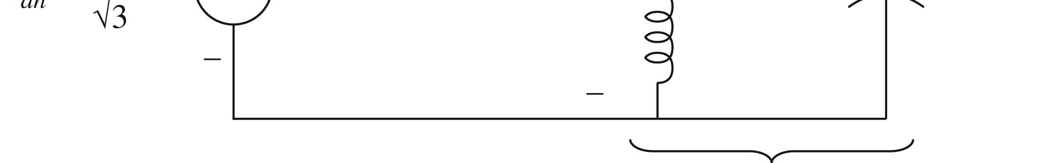
taken as a reference, the per-phase equivalent circuit is shown below:
Total impedance viewed from the input terminals is
The three-phase complex power supplied = 1 3*1800WSVI==
1800W P = and 0VAR Q = delivered by the sending-end source
18 ©
Cengage Learning®. May not be scanned, copied or duplicated, or posted to a publicly accessible website, in whole or in part. ( )( ) * 3
2017
33120.13024.0266.87
ana SVI j φ ==∠−°∠+° =∠°=+
φφ
( )
pfSSφφ =°===
336923W;5192VAR;PQ
==
33 cos36.870.8Lagging;8654VA
(b)
aba VI=∠°=∠−°∠−°
() 2 6045 2015 3 j Zj==−Ω
1203 1 3 120V V ==
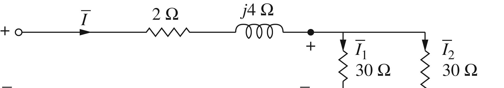
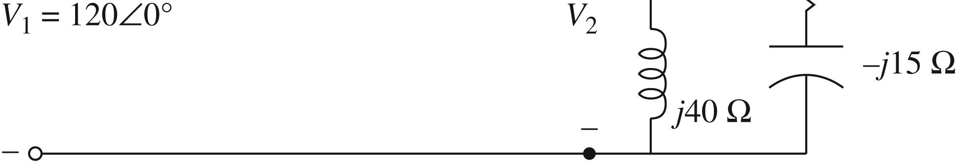
( )( ) ()() 1 30402015 242422424 30402015 1200 50A 24 jj Zjjj jj V I Z +− =++=++−=Ω ++− ∠° ===∠°
(b)Phase voltage at load terminals ( )( ) 2
The line voltage magnitude at the load terminal is
(c) The current per phase in the Y-connected load and in the equiv.
of the
The phase current magnitude in the original ∆-connected load
(d)The three-phase complex power absorbed by each load is
The three-phase complex power absorbed by the line is
The sum of load powers and line losses is equal to the power delivered from the supply:
2.44 (a) The per-phase equivalent circuit for the problem is shown below: Phase voltage at the load terminals is 2
19 ©
Cengage Learning®. May not be scanned, copied or duplicated, or posted to a publicly accessible website, in whole or in part.
2017
12002450
11020111.810.3V j =−=∠−°
Vj=∠°−+∠°
( ) LOAD3111.8193.64V LL V ==
2 1 1 2 2 2 122.23663.4A 424.47226.56A V Ij Z V Ij Z ==−=∠−° ==+=∠°
Y
∆-load:
() 2 4.472 2.582A 33 ph I I ∆ ===
* 121 * 222 3430W600VAR 31200W900VAR SVIj SVIj ==+ ==−
( ) ( ) 22 3324(5)150W300VARLLL SRjXIjj =+=+=+
( ) ( ) ( ) 12 4506001200900150300 1800W0VAR L SSSjjj j ++=++−++ =+
22003 2200V
()
3 560.10.7070.70713252839666036.87kVA R
φ
3 V == taken as Ref. Total complex power at the load end or receiving end is
( )
Sjj
=++=+=∠°
With phase voltage 2V as reference,
Phase voltage at sending end is given by
The magnitude of the line to line voltage at the sending end of the line is

(b)The three-phase complex-power loss in the line is given by
(c) The three-phase sending power is
Note that
(b)The ammeter reads zero, because in a balanced three-phase system, there is no neutral current.
20 © 2017 Cengage Learning®. May not be scanned, copied or duplicated, or posted to a publicly accessible website, in whole or in part.
() () * 3 * 2 660,00036.87 10036.87A 3322000 RS I V φ ∠−° ===∠−° ∠°
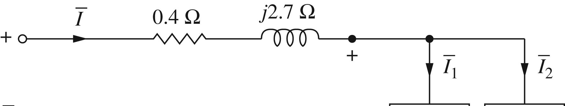
( )( ) 1 220000.42.710036.872401.74.58VVj=∠°++∠−°=∠°
( ) ( ) 11332401.74160V LL VV===
() ()( ) ()()2 222 3 3330.410032.7100 12kW81kVAR L SRIjIj j φ =+×=+ =+
() ( )( ) * 1 3 332401.74.5810036.87 540kW477kVAR S SVI j φ ==∠°∠° =+
()
333 SRL SSSφφφ =+ 2.45 (a) () 325.00110 30.07A 33480 S S LL S I V × ===
() ()
2.46 (a)
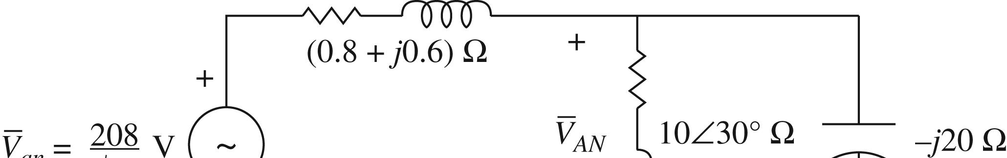
21 © 2017 Cengage Learning®. May not be scanned, copied or duplicated, or posted to a publicly accessible website, in whole or in part. Using voltage division: /3 (/3) ANan LINE Z VV ZZ ∆ ∆ = + () ()() 2081030 0 10300.80.6 3 120.091030 1200.930 9.465.610.9930.62 109.30.62V j j ∠° =∠° ∠°++ ∠° ∠° == +∠° =∠−° Load voltage = ( ) 3109.3189.3VLine-to-Line ABV == (b) ( )1030||20 11.5470 eq Zj =∠°− =∠°Ω () () 11.547 2083 11.5470.80.6 1386.7 112.22.78V 12.3622.78 eq ANan eqLINE Z VV ZZ j = + = ++ ==∠−° ∠° Load voltage Line-to-Line ( ) 3112.2194.3 V ABV == 2.47 (a) ()() 3 1 1 1510 cos0.823.5336.87A 84600.8 GI × =∠−=∠−° ()() 111 460 01.41.623.5336.87 3 216.92.73VLine to Neutral LGLINEG VVZIj =−=∠°−+∠−° =∠−° LoadVoltage3216.9375.7VLine to line LV ==
22 © 2017 Cengage Learning®. May not be scanned, copied or duplicated, or posted to a publicly accessible website, in whole or in part. (b) ()() 3 1 3010 2.73cos0.857.6339.6A 3375.70.8 LI × =∠−°−=∠−° 21 57.6339.623.5336.87 GLG III=−=∠−°−∠−° 34.1441.49A=∠−° ( )( ) 222 216.92.730.8134.1441.49 GLLINEG VVZIj =+=∠−°++∠−° 259.70.63V =∠−° Generator 2 line-to-line voltage ( ) 2 3259.7 GV = 449.8V = (c) ( )( ) * 2 2233259.70.6334.1441.49GG GSVI==∠−°∠° 33 20.121017.410 j =×+× 2220.12kW;17.4kVAR;Both delivered GG PQ== 2.48 (a) (b) cos31.320.854Lagging pf =°= (c) () 326.9310 32.39A 33480 L L LL S I V × === (d) () () 2 3 2 3 1410VAR3/ 3480 49.37 1410 CLLL QQVX X ∆ ∆ ==×= ==Ω × (e) 3 /480/49.379.72A 2310 27.66A 33480 CLL L LINE LL IVX P I V ∆ === × ===
2.49 (a) Let YABC ZZZZ === for a balanced Y-load
23 © 2017 Cengage Learning®. May not be scanned, copied or duplicated, or posted to a publicly accessible website, in whole or in part.
ABBCCAZZZZ ∆ ===
equations in Fig. 2.27 222 3 YYY Y Y ZZZ ZZ Z ∆ ++ == and 2 3 Y ZZ Z ZZZ ∆∆ ∆∆∆ == ++ (b) ( )( ) ()() ()() 1025 50 102025 10202025 40;100 55 A B C jj Zj jjj jjjj ZjZj jj ==−Ω +− ==Ω==−Ω 2.50
delta by the equivalent WYE: 2 3 Y Zj=−Ω
Using
Replace
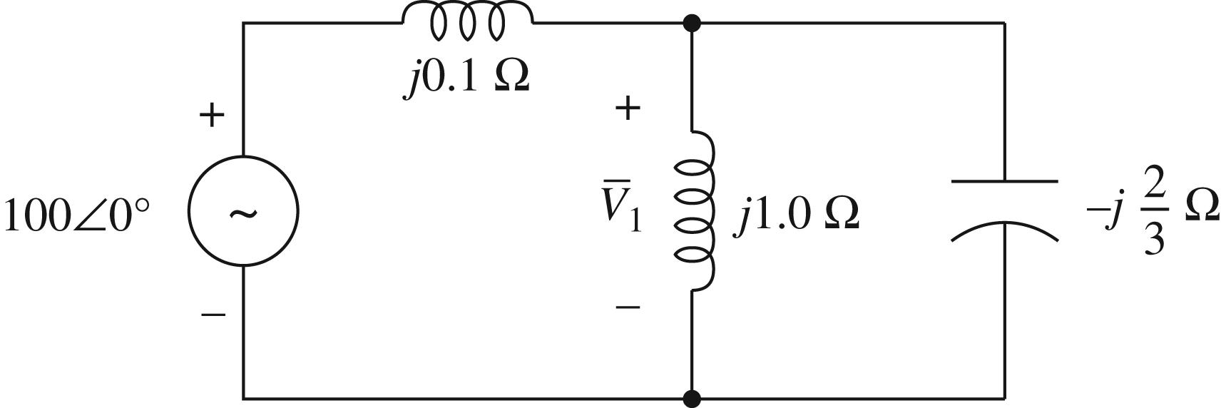
Noting that 2 1.02 3 jjj −=− , by voltage-divider law, () 1 2 10001050 20.1 j V jj =∠°=∠° −+ 1()1052cos(0)148.5cosV ttt υωω ∴=+°=← In order to find 2()it in the original circuit, let us calculate ABV ′′ 30 3173.230 j ABANBNAN VVVeV ° ′′′′′′′′ =−==∠° Then 173.230 86.6120 2 AB I j ′′ ∠° ==∠° ( ) 2()86.62cos120 itt ω ∴=+° ( ) 122.5cos120A tω =+°←
Per-phase equivalent circuit is shown below:
24 © 2017 Cengage Learning®. May not be scanned, copied or duplicated, or posted to a publicly accessible website, in whole or in part. 2.51 On a per-phase basis ()() 1 1 1501205040kVA 3 Sjj =+=+ ( ) () 3 1 504010 2520A 2000 Note:PFLagging j Ij ∴==− Load 2: Convert ∆ into an equivalent Y ()() () 2 2 1 150485016 3 20000 38.117.74 5016 36.2911.61A Note:PFLeading Y Zjj I j j =−=−Ω ∠° ∴==∠° =+ () () () 1 3 1 perphase1200.6120sincos0.62432kVA 3 Sjj =×−=− ( ) () 3 3 243210 1216A 2000 Note:PFLeading j Ij + ∴==+ Total current drawn by the three parallel loads 123 T IIII =++ ( ) 73.297.61A Note:PFLeading TOTAL Ij =+ Voltage at the sending end: ( )( )2000073.297.610.21.0 AN Vjj =∠°+++ 2007.0574.812008.442.13V j =+=∠° Line-to-line voltage magnitude at the sending end = ( ) 32008.443478.62V=← 2.52 (a) Let ANV be the reference: 2160 024000V 3 ANV =∠°∠° ≃ Total impedance per phase ( ) ( ) ( )4.790.31510 Zjjj =+++=+Ω 24000 Line Current214.763.4A 510 A I j ∠° ∴==∠−°=← + With positive A-B-C phase sequence, 214.7183.4A;214.7303.4214.756.6ABC II=∠−°=∠−°=∠°←
25 © 2017 Cengage Learning®. May not be scanned, copied or duplicated, or posted to a publicly accessible website, in whole or in part. (b) ( ) ( )( ) () () 24000214.763.40.31 24000224.159.92179.238.54 2179.51.01V 2179.5121.01V;2179.5241.01V AN LOAD BN CN LOAD LOAD V j j VV ′ ′ ′ =∠°−∠−°+ =∠°−∠°=− =∠−°← =∠−°=∠−° □ □ (c) ( ) ( )( ) /Phase2179.5214.7467.94kVA ANA LOAD SVI ′ ===← Total apparent power dissipated in all three phases in the load ( ) 3 3467.941403.82kVA LOAD S φ ==← Active power dissipated per phase in load = ( ) 1 LOAD Pφ ( )( ) ( ) 2179.5214.7cos62.39216.87kW =°=← ( ) 3 3216.87650.61kW LOAD P φ ∴==← Reactive power dissipated per phase in load = ( ) 1 LOAD Q φ ( )( ) ( ) 2179.5214.7sin62.39414.65kVAR =°=← ( ) 3 3414.651243.95kVAR LOAD Q φ ∴==← (d)Line losses per phase ( ) ()2 1 214.70.313.83kW LOSS Pφ ==← Total line loss ( ) 3 13.83341.49kW LOSS P φ =×=←
26 © 2017 Cengage Learning®. May not be scanned, copied or duplicated, or posted to a publicly accessible website, in whole or in part. Power System Analysis and Design SI Edition 6th Edition Glover Solutions Manual Visit TestBankDeal.com to get complete for all chapters
