(a) What is the degree of freedom for the QoLCat effect?
The degree of freedom for the QoLCat effect is 4-1=3.
(b)What is the total sum of square (SS) for severity that is explained by QoLCat?
The total sum of square for severity that is explained by QoLCat is 1153.659.
(c) What is the mean square (MS) for severity that is explained by QoLCat?
The mean square (MS) for severity that is explained by QoLCat is 384.553.
(d)What is the degree of freedom for the error term?
The degree of freedom of the error term is 799-4= 795.
(e) What is the mean square error (MSE)?
The mean square error is 10.750.
(f) Conduct a hypothesis test to assess the effect of QoLCat on severity.
H o= QoLCat is not statistically significant factor on severity.
H1= QoLCat is a statistically significant factor on severity.
F= 35.772; p-value <0 .000
Alpha = 0.05, H0 can be rejected since the p-value <0.000, suggesting that there is evidence that QoLCat is a statistically significant factor on severity.
2. Obtain the estimated mean of severity for each of the four QoL levels.
Descriptives
95% Confidence Interval for Mean Mini mum Maximu m
Std. Deviat ion Std. Error
.793 14.63 19.67 2.018
BetweenCompon ent Variance Lower Bound Upper Bound 1 112 19.17 2.956 .279 18.62 19.72 12 26 2 312 17.76 3.205 .181 17.41 18.12 4 27 3 272 16.38 3.125 .189 16.01 16.75 9 26 4 103 15.14 4.126 .407 14.33 15.94 5 27 Total 799 17.15 3.486 .123 16.91 17.39 4 27 Model Fixed Effects 3.279 .116 16.92 17.38 Rando m Effects www.statisticsassignmenthelp.com
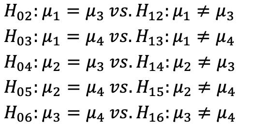
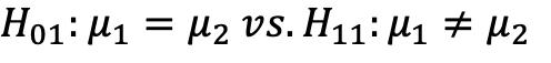
All p-values listed above are below 0.05. Reject H0.All the pair listed (1-2,1-3,1-4,21,2-3,2-4,3-1,3-2,3-4,4-1,4-2,4-3) have a statistically significantdifference in the mean of severity. Mean differences and CI for each is listed above.
Question 2: Using Two-way ANOVA model to test if Treatment and QoLCat are a statistically significant factors on severity
1. In the two-way ANOVA model, you first include the two main effect and the interaction between the two main effects.
Type III Sum of Squares df Mean Square F Sig. Partial Eta Squared Noncent. Parameter Corrected Model 2323.571a 7 331.939 35.595 .000 .240 249.165 Intercept 179210.294 1 179210.294 19217.40 0 .000 .960 19217.400 QOLCat 1065.544 3 355.181 38.087 .000 .126 114.262 Treatment 854.473 1 854.473 91.628 .000 .104 91.628 QOLCat * Treatment 177.312 3 59.104 6.338 .000 .023 19.014 Error 7376.406 791 9.325 Total 244709.000 799 Corrected Total 9699.977 798
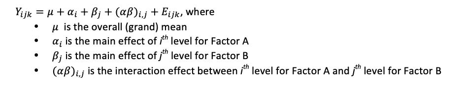
In this case alphai= QOLCat, betaj = Treatment and (alpha*beta)ij is the interaction
effect between QOLCat and treatment.
(a) Conduct an overall F test to examine if this ANOVA model is significantly better than the null model.
H o= The ANOVA model is not significantly better than the null model.
H1= The ANOVA model is significantly better than the null model.
F= 35.595; p-value <0 .000
Alpha = 0.05, H0 can be rejected since the p-value <0.000, suggesting that the ANOVA model is significantly better than the null model.
(b) In this ANOVA model, what are the degrees of freedom for (i) Treatment, (ii) QoLCat, (iii) the interaction term, and (iv) the error term?
The degrees of freedom are the following:
•Treatment = 1
•QOLCat = 3
•The interaction term (QOLCat * Treatment) = 3
•The error term = 791
Type III Sum of Squares df Mean Square F Sig. Partial Eta Squared Noncent. Parameter Corrected Model 2323.571a 7 331.939 35.595 .000 .240 249.165 Intercept 179210.29 4 1 179210.2 94 19217.4 00 .000 .960 19217.400 QOLCat 1065.544 3 355.181 38.087 .000 .126 114.262 Treatment 854.473 1 854.473 91.628 .000 .104 91.628 QOLCat * Treatment 177.312 3 59.104 6.338 .000 .023 19.014 Error 7376.406 791 9.325 Total 244709.00 0 799 Corrected Total 9699.977 798
interaction
Alpha = 0.05, H0 can be rejected since the p-value <0.000, suggesting that the interaction term (QOLCAT * Treatment) is statistically significant.
3. How many terms should be included in the final two-way ANONA model? What are they?
All three terms should be included in the model because they are all statistically significant with p- values <0.000. The names of these terms are QOLCat, treatment, and QOLCAT * Treatment (the interaction term.
4. Conduct the type III F test for two main effects (Treatment, QolCat) in the final ANOVA model.
Alpha = 0.05, H0 can be rejected since the p-value <0.000, suggesting that QOLCatis statistically significant.
H o= The term treatment is not statistically significant.
H1= The term treatmentis statistically significant.
F= 91.628; p-value <0 .000
Alpha = 0.05, H0 can be rejected since the p-value <0.000, suggesting that treatment is statistically significant.
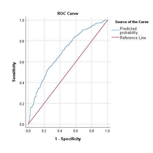
Using Cook’s distance point, the maximum value shows 0.076, which is less than 1 suggesting there are no serious influence points in the dataset.
(b).What is the Pearson’s correlation coefficient between the linear term (QOL) and the quadratic terms (QOL2)?
Correlations
Severity QOL qol2
Pearson Correlation Severity 1.000 -.472 -.483 QOL -.472 1.000 .989 qol2 -.483 .989 1.000
The Pearson’s correlation coefficient between the linear term and quadratic term is 0.989.
(c)Using rule of thumb for variation inflation factor (VIF) to see if there is a collinearity issue.
Model
Unstandardized Coefficients
Standardize d Coefficients
t Sig. B Std. Error Beta VIF
1 (Constant) 24.412 .493 49.542 .000 QOL -.134 .009 -.472 -15.110 .000 1.000
2 (Constant) 18.895 1.587 11.905 .000 QOL .079 .059 .279 1.343 .180 44.988 qol2 -.002 .001 -.759 -3.654 .000 44.988
With VIF> 10, there is a collinearity issue between QOL and QOL2. 2.If there is a severe collinearity issue, what is the remedy? Rerun your model using this method and then test significances of the corresponding linear and quadratic terms.
Model
Unstandardized Coefficients
Standardiz ed Coefficient s
T Sig. B Std. Error Beta VIF
1 (Constant ) 17.150 .109 157.60 6 .000 qolcenter -.134 .009 -.472 -15.110 .000 1.000 2 (Constant ) 17.444 .135 129.45 3 .000 qolcenter -.133 .009 -.46815.080 .000 1.001 qolcenter 2 -.002 .001 -.113 -3.654 .000 1.001 Since this is a quadratic equation, we must center the predictor/ independent variable by subtracting the mean from each observation using the equation below ��=0+1− +2− 2+ ���������������� Using the new terms, the VIF for qolcenter and qolcenter2 is 1.001, which is less than ten. This solves the issue of collinearity.
Model
Sum of Squares df Mean Square F Sig.
1 Regression 2159.975 1 2159.975 228.316 .000b Residual 7540.002 797 9.460 Total 9699.977 798 2 Regression 2284.349 2 1142.175 122.602 .000c Residual 7415.628 796 9.316 Total 9699.977 798
a. Dependent Variable: Severity b. Predictors: (Constant), qolcenter c. Predictors: (Constant), qolcenter, qolcenter2
H o= The linear (qolcenter) and quadratic terms (qolcenter2) does not significantly add to the model. H1= The linear (qolcenter) and quadratic terms (qolcenter2) does significantly add to the model.
F= 122.602 and p-value <0.000 At alpha =0.05, H0 can be rejected since the p-value <0.000, the linear (qolcenter) and quadratic terms (qolcenter2) does significantly add to the model. The final model of the data should be
(a)Conduct an overall F test to examine if the model is significantly better than the null model.
Type III Test (Testing against the Null) a
Source Numerator df Denominat or df F Sig. Intercept 1 799 938.84 8 .000 Treatme nt 1 799 5.750 .017 a. Dependent Variable: Hosp1yr. H o= The model isnot statistically better than the null. H1= The model is statistically better than the null . F= 5.750; p-value =0.017 Alpha = 0.05, H0 can be rejected since the p-value =0.017, suggesting the model (with terms)is statistically better than the null. (b) What are the values of AIC and deviance (-2log likelihood) for the model?
Unadjusted odds ratio for hospitalization between patients treated with the experimental drug and the standard of care is 1.417 CI 95% (1.063, 1.889).
2.Test if gender is a confounder for the relationship between hospitalization and Treatment.
B S.E. Wald df Sig.
Step 1a Treatmen t(1) .367 .148 6.142 1 .013 Male(1) -.573 .144 15.794 1 .000 Intercept .322 .117 7.574 1 .006
a. Variable(s) entered on step 1: Treatment, Male.
B S. E. Wald df Sig.
Step 1a Treatment (1) .349 .14 7 5.658 1 .017 Intercept .033 .09 1 0.132 1 .717
a. Variable(s) entered on step 1: Treatment.
H o= Gender isnot a cofounder.
H1= Gender is a cofounder. Gender is not a cofounder because the percent change is beta is within the acceptable range, less than 10 % as measured by beta one (0.367-0.349/0.349) *100= 5.16%
2. Test if gender is an effect modifier for the relationship between hospitalization and Treatment.
B Std. Error Wald df Sig.
Step 1a Treatment( 1) .357 .217 2.700 1 .101 Male(1) -.581 .183 10.034 1 .002 Male*Treat ment .02 .297 0.005 1 .946 Constant .327 .131 6.255 1 .012
a. Variable(s) entered on step 1: Treatment, Male, Male* Treatment.
H o= Gender isnot an effect modifier for the relationship between hospitalization and treatment.
H1= Gender is aneffect modifier for the relationship between hospitalization and treatment.
Wald= 0.005; p-value =0.946 Alpha = 0.05, H0fails to be rejected since the p-value =0.946, since gender isnot an effect modifier for the relationship between hospitalization and treatment.
4.Conduct a multiple logistic regression model for the relationship between Treatment & hospitalization adjusting for the following covariates: age, Hispanic race, and residency (urban/rural). (5 pts)
Model Fitting Information
Model Fitting Criteria Likelihood Ratio Tests AIC BIC -2 Log Likelihood ChiSquare df Sig. Intercept Only 1090.7 37 1095.420 1088.737 Final 1024.1 76 1047.593 1014.176 74.561 4 .000
Model
Goodness-of-Fit ChiSquare df Sig. Pearson 782.596 761 .286 Devianc e 1001.464 761 .000
Effect
Pseudo R-Square
Cox and Snell .089 Nagelkerke .119 McFadden .068
Likelihood Ratio Tests
Model Fitting Criteria
Likelihood Ratio Tests
AIC of Reduced Model BIC of Reduced Model
-2 Log Likelihood of Reduced Model Chi-Square df Sig.
Intercept 1024.176 1047.593 1014.176a .000 0 . age1 1032.493 1051.226 1024.493 10.317 1 .001 Treatment 1031.889 1050.622 1023.889 9.713 1 .002 Hispanic 1077.713 1096.447 1069.713 55.537 1 .000 Urban 1034.772 1053.505 1026.772 12.596 1 .000
The chi-square statistic is the difference in -2 log-likelihoods between the final model and a reduced model. The reduced model is formed by omitting an effect from the final model. The null hypothesis is that all parameters of that effect are 0. a. This reduced model is equivalent to the final model because omitting the effect does not increase the degrees of freedom.
Hosp1yra B Std. Error Wald df Sig. 0 Intercept -3.846 .829 21.52 9 1 .000 age1 .051 .016 10.18 0 1 .001 [Treatme nt=0] .480 .155 9.584 1 .002 [Treatme nt=1] 0b . . 0 . [Hispani c=0] 1.312 .185 50.23 4 1 .000 [Hispani c=1] 0b . . 0 . [Urban= 0] -.622 .177 12.30 2 1 .000 [Urban= 1] 0b . . 0 .
(a) Conduct the partial Wald test for the treatment effect on hospitalization in this model.