


T = Z/ √U/n a Student’s t random variable with n degrees of freedom.

Find the density function of T
Solution:
• The density of Z is fZ(z) =
• The density of U is
• Because Z and U are independent their joint density is fZ,U (z, u) = fZ(z)fU (u)
• Consider transforming (Z,U) to (T, V ), where
T = Z/ √U/n and V = U,
computing the joint density of (T, V ) and then integrating out V to obtain the marginal density of T.
-Determine the functions g(T, V ) = Z and h(T, V ) = U

Then the joint density of (T, V ) is given by fT,V (t, v) = fZ,U (g(t, v), h(t, v)) × J where J is the Jacobian of the transformation from (Z,U) to (Z,U).


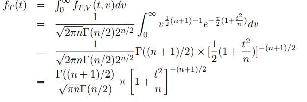
The joint density of (T, V ) is thus
Integrate over v to obtain the marginal density of T:


The integral factor can be evaluated by recognizing that it is identical to integrating a Gamma(α, λ) density function apart from the normalization constant, with α = (n + 1)/2 that is which gives

Finally we can write
2. Suppose the random variable X has a t distribution with n degrees of freedom.
(a). For what values of n is the variance finite/infinite.
(b). Derive a formula for the variance of X (when it is finite).
Solution:
(a). For the variance of the t distribution to be finite it must have a finite second moment:

The integrand of this second moment calculation is proportional to
The integral of this integrand thus converges if and only if (1 − n) < (−1), which is equivalent to n > 2.


(b). If n > 2, then the variance of T is finite. For such n, the mean of T exists and is zero, so writing T = Z/ U/n for independent Z N(0, 1) and U ∼
The expectation can be computed directly for n > 2. U (Note that the formula is undefined for n = 2 and gives negative values for n < 2)
3. 6.4.4. Also, add part (c) answer the question if the random variable T follows a standard normal distribution N(0, 1). Comment on the differences and why that should be.
Solution: We are given that T follows a t7 distribution. The problem is solved by finding an expression for t0 in terms of the cumulative distribution function of T.
(a). To find the t0 such that P(|T| < t0) = .9 this is equivalent to P(T < .95), which is solved in R using the function qt() – the quantile function for the t distribution
> args(qt)
function (p, df, ncp, lower.tail = TRUE, log.p = FALSE)
>qt(.95,df=7)
[1] 1.894579
So, t0 = 1.894579.
(b). P(T > t0) = .05 is equivalent to P(T ≤ t0) = 1 − .05 = .95. This is the same t0 found in (a).
> args(qt)
function (p, df, ncp, lower.tail = TRUE, log.p = FALSE)
> qt(p=.95, df=7)
[1] 1.894579
# Which is equivalent to > qt(p=.05, df=7, lower.tail=FALSE)
[1] 1.894579
(c). For the standard normal distribution we use qnorm() – the quantile function for the Normal(0, 1) distribution
> args(qnorm)
function (p, mean = 0, sd = 1, lower.tail = TRUE, log.p = FALSE)
NULL > qnorm(.95) [1] 1.644854
> qnorm(p=.05, lower.tail=FALSE)
[1] 1.644854
So for both parts (a) and (b) t0 = 1.644854 for the N(0, 1) r.v. versus t0 = 1.894579 for the t distribution with 7 degrees of freedom. The t0 values are larger for the t distribution indicating that the t distribution has heavier tail areas than the Normal(0, 1) distribution. This makes sense because the t distribution equals a Normal(0, 1) random variable divided by a random variable with expectation equal to 1 but positive variance. The possibility of the denominator of the t ratio being less than 1 increases the probability of larger values.
4. Problem 8.10.10. Use the normal approximation of the Poisson distribution to sketch the approximate sampling distribution of λˆ of Example A of Section 8.4. According to this approximation, what is
where λ0 is the true value of λ.
Solution: In the example, the estimate
The X1, . . . , Xn are assumed to be i.i.d. (independent and identically distributed) Poisson(λ0) random variables with E[Xi] = λ0 and V ar[Xi] = λ0
By the Central Limit Theorem
The approximate sampling distribution of λˆ is thus a Normal distribution centered λ0
standard deviation equal to
For the probability computations:

Using R and the function pnorm we can compute the desired values:
In Example D of Secton 8.4, the method of moments estimate was found to be αˆ = 3X. In this example, consider the sampling distribution of α. ˆ
(a). Show that E(ˆα) = α, that is, that the estimate is unbiased.
(b). Show that V ar(ˆα) = (3 − α2)/n.
(c). Use the central limit theorem to deduce a normal approximation to the sampling distribution of α. ˆ
According to this approximation, if n = 25 and α = 0, what is the P(|αˆ| > .5). Solution
The sample of values X1, . . . , Xn giving X are i.i.d. with density function
with parameter α : −1 ≤ α ≤ 1. (The values are such that xi = cos(θi), where θi is the angle at which electrons are emitted in muon decay.)
(a). Since the Xi are i.i.d
It follows that:
(c) By the central limit theorem, for true parameter α = α0, it follows that


