Industry Threshold

Thin-Bed Tuning-Frequency: Thickness Estimation

Victor Aarre - Geophysics Advisor - schlumberger

Introduction It is well known in the industry that seismic reflections from geological interfaces in the earth’s interior interfere with each other. This interference may either be constructive or destructive. The seismic wavelet is, according to the Fourier theorem, the sum of a number of individual frequencies, where each frequency has its own amplitude and phase. When a seismic wavelet is reflected from two neighboring reflectors (defined as the top and bottom of a thin bed), the amplitude spectrum of the reflected wavelet will hence be different from the spectrum of the original wavelet. This is because each frequency in the wavelet will have different amplitude, due to the interference between the reflectors ( I.e. the two reflectors act as a filter). By examining the spectrum of the reflected wavelet, it is hence, in some cases, possible to infer the presence and thickness of thin beds in the underground. These thin beds are often of great commercial interest for the energy industry, because the most common scenario is a sand body embedded in a shale host rock. A sand body is often porous and permeable, making it a perfect reservoir rock for hydrocarbons. Shale rocks are most often not permeable (unless the rock is fractured), and are hence excellent reservoir cap (and source) rocks, keeping the hydrocarbons in place in the embedded sand body.

Prior Art There are a lot of prior arts in this domain. The most famous approach was discovered, and patented, by BP. The commercial name of their approach is “The Tuning Cube”. That invention was further elaborated on in a paper, written by K. Marfurt and R. Kirlin, in the Geophysics journal in 2001. That paper is an excellent introduction to the general scientific topic. What’s common for all existing methods I know of (for thin-bed detection through spectral decomposition) is that those methods attempt to infer the presence of thin beds through studies of the amplitude spectrum of the reflected waveform. This is a challenge; because the amplitude of the individual frequencies in the source wavelet is not equal (i.e. the amplitude spectrum of the wavelet is not “white” or “flat”). This means that the reflected seismic must become spectrally balanced before the tuning analysis begins. This spectral balancing step is complicated, at least when we do not have any wells available for joint log/seismic wavelet estimation, and we hence need to use blind/statistical methods for the spectral balancing step. components one want to analyze. This number is in general dependent on the sample rate (which determines the maximum frequency, called Nyquist frequency) and the number of samples in the trace (which determines the number of spectral components which are required to fully represent the input trace).

Fig.2 - This is the amplitude of the individual spectral components

Description of the Invention Including Examples and Drawings

In Fig 2, Note that the lowest frequencies (to the left) and the highest frequencies (to the right) are very weak, compared to the amplitudes in the center of the spectrum. It will be impossible to establish spectral high’s or low’s without first doing a spectral balancing step. This is the step we aspire to avoid with this invention. Note that the amplitude of each spectral component is, in general, identical to the Envelope (which is often also known as the “Reflection Strength”) of that spectral component.

Fig.1 - One vertical section intersecting a 3D seismic cube

We will perform the analysis independently on each trace in the cube, and the method is hence not restricted to 3D seismic. It works equally well for 2D and 1D seismic data. The method is actually not dependent on seismic at all. It can work on any time series of any data (e.g. voice, radar, x-ray, etc.). For each trace, replicate it into the desired number of spectral

Fig.4 - This is the instantaneous frequency for each spectral component

Instantaneous Frequency is per definition equal to (1/360) * d/ dt (instantaneous phase), and the unit is (of course) Hz (i.e. oscillations per second).

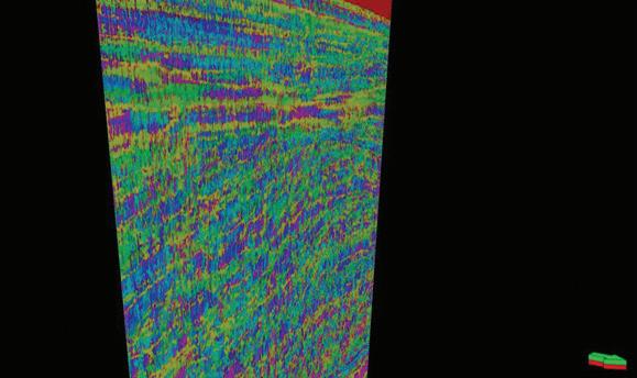
Fig.5 - The corresponding “tuning thickness” result

Summary of the Method

The reflected seismic must become spectrally balanced before the tuning analysis begins. This spectral balancing step is complicated, at least when we do not have any wells available for joint log/seismic wavelet estimation and we hence need to use blind/statistical methods for the spectral balancing step. The summary of this invention is a practical and simple way to estimate tuning frequency through an investigation of the phase spectrum, instead of the amplitude spectrum (as done by all prior art), of the reflected seismic. This removes the dependency of the spectral balancing step, which is required by all existing methods.

The steps are as follows, for each individual trace in a 3D seismic volume:

1) Split the trace into a set of individual spectral components, each with its own unique frequency F.

2) Calculate instantaneous frequency Fi for each spectral component (please note that instantaneous frequency is the derivative of instantaneous phase; this means that the instantaneous frequency is totally un-correlated to the seismic amplitude of the spectral component).

3) We know that, in theory, the instantaneous frequency Fi for each sample in the spectral component F should be identical to F. This will not be the case for samples where we have destructive interference (because we do not have a reflected signal there for that spectral component, and the phase will hence be undefined, as it’s a singularity), and the spectral component Fi will hence be different from F.

4) Quantify the difference Di between Fi and F, and use this as an indicator measure of destructive interference, for each spectral component F.

5) For each sample in the input trace: search for the spectral component Ft where the difference Di is maximum for that sample. Ft will be the tuning frequency for that sample. The search may optionally be bound between user-provided limit frequencies F min and F max .

6) The limit frequencies F min and F max can optionally be estimated from Di for each spectral component, and may possibly be estimated as a smoothly time-varying function. This is because Di will be highly chaotic for the lowest and highest frequencies. These are the frequencies outside the bandwidth of the seismic wavelet. We can hence use a measure of chaos in Di to establish where the frequencies start to become reliable, and hence determine the limits of the useful frequency spectrum for the input seismic data.

7) Optionally calculate the tuning thickness T from the tuning frequency Ft for each sample in the input trace. We know that the tuning frequency is inferred from destructive interference, and that the most likely cause for destructive interference is a thin bed with equal, but opposite polarity, reflectors. We can hence use this equation: T = 1/ Ft.

Principal Components Methodology: A Novel Approach to Forecast Production

Dr. Ibukun Makinde - Researcher - University of Houston

The oil and gas industry is in need of quick and simple techniques of forecasting oil and gas production. Existing traditional decline curve analysis (DCA) methods have been limited in their ability to satisfactorily forecast production from unconventional liquid rich shale reservoirs. This is due to several causes ranging from the complicated production mechanisms to the ultra-low permeability of shale. The use of hybrid (combination) DCA models (SPE-179964-MS) have been able to improve results significantly.

However, complexities associated with these techniques can still make their application quite tedious without proper diagnostic plots, correct use of model parameters and some knowledge of the production mechanisms involved. Therefore, the Principal Components Methodology (PCM) provides us with a way to bypass a lot of these difficulties. PCM is a data-driven method of forecasting based on the statistical technique of principal components analysis (PCA). A pictorial representation of the PCM workflow is shown below:

The procedure for forecasting production using PCM consists of the following steps:

1- Generate representative collection of well production data through simulation for time t n and construct a m × n matrix Z from the representative data.

m – number of wells n – length of production history (time) q i (i = 1…m) are the oil/gas rates of well i over time.

2- Apply principal components analysis to the representative well data through the use of singular value decomposition to obtain the principal components.

(Singular values – in decreasing order from top to bottom of diagonal matrix S).

R – number of sets of principal components (PCs) to be used in forecasting

βk – PC multiplier

3- Given wells with limited production history, use the least squares regression method to identify best estimates for β k (PC multiplier), which would be β k , with the following formula:

An example of a PCM forecast (light blue dash line) in comparison to hybrid DCA model forecasts for multi-stage hydraulically fractured horizontal well with 6 months to 3 years of production history are shown graphically below:

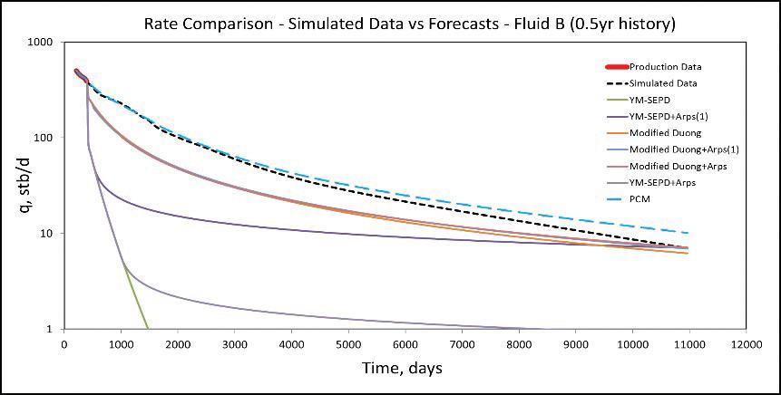
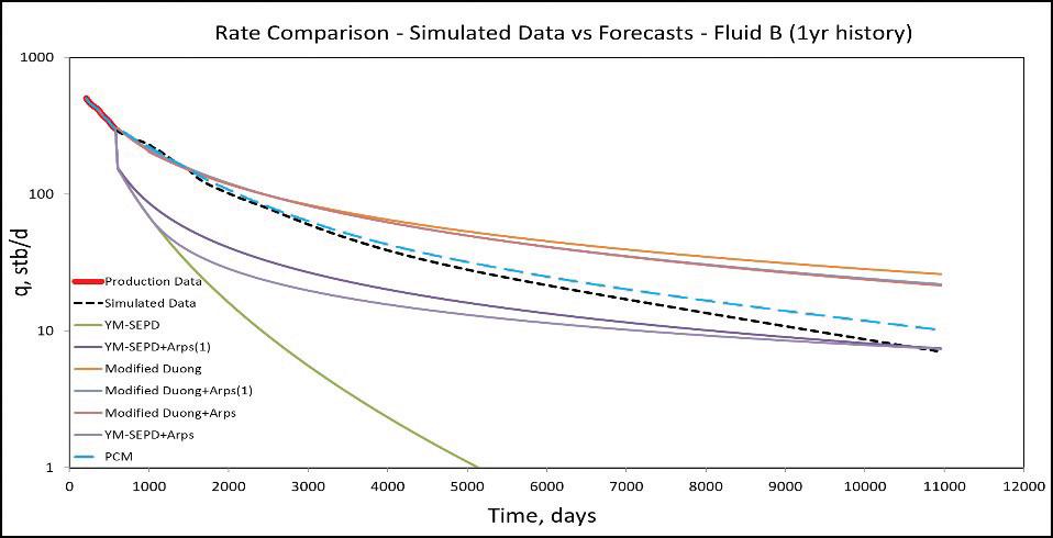
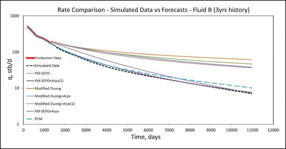
From results, it is observed that YM-SEPD hybrid models severely underestimate production with production history less than 2 years. Also, Modified Duong hybrid models overestimate production in most cases. However, the Principal Components Methodology (PCM) forecasts are consistently good regardless of the amount of historical production data available.

Advantages of PCM over empirical and analytical forecasting methods are:

1. It eliminates the need to determine vital decline curve analysis (DCA) model parameters like the hyperbolic decline exponents (b values);

2. Diagnostic plots are not necessary prior to forecasting with PCM;

3. It avoids the complication of switching from one DCA model to another, as is the case with hybrid (combination) DCA models;

4. It does not involve complex and rigorous calculations;

5. It is possible to determine the time (point) of switch to Arps after careful analyses of the inverse MBT vs. time plot, the Yu plot and corresponding diagnostic plots - this time of switch may be the “true” start of boundary dominated flow;

6. The Duong model and its hybrid alternatives overestimate production in shale volatile oil reservoirs - overestimation increases with shorter production histories. These inaccuracies are a result of the nature of data due to early change from linear flow to transition flow regime, which contradicts the assumption of long-term linear (or bilinear) flow in the original Duong model;

7. The Duong hybrid models led to better forecasts than the original Duong model but still overestimate production (in most cases) in comparison to results from the YM-SEPD and its hybrid models;

8. The YM-SEPD hybrid models led to better production forecasts in all cases, but were limited by lack of production data beyond the minimum of 2-3 years required for best application of the YM-SEPD model. And the use of the Duong model to forecast 2nd and 3rd year pseudohistorical data to generate n and T, did not lead to «best» results (except when hybrid alternatives were applied) because of the limitations of the original Duong model;

9. Even though further research is needed in the area of solution gas production forecasting, it is possible to forecast solution gas production from shale volatile oil reservoirs with some measure of accuracy, provided there are sufficient data available;

10. A proposed Modified Duong model helps to alleviate the problem of serious overestimate of future production by the original Duong model. A hybrid model of Modified Duong and then Arps can lead to even better forecasts, but additional work (in progress) will be required to evaluate this model.