Industry Threshold

Stress Profiling With Microfracturing and Sonic Logs in Antelope Shale

Mayank Malik - Formation Testing Expert at Chevron, Houston, Texas

Shale development has changed the landscape of hydrocarbon production and dynamics. “Getting it right”, however, requires picking optimum lateral landing points and knowing the stress profile across the reservoir. The following article describes a case study on successful integration of microfracture testing with sonic logs in Antelope Shale. Antelope Shale is a silica-rich diatom deposition, which produces from reservoirs in all three silica phases: Opal A (Diatomite), Opal CT, and Quartz. While the Opal A has heavy oil that has been successfully produced, Opal CT and Quartz resources have largely been locked. Due to recent advancement in unconventional completions and hydraulic fracturing, there is a renewed interest in CT/ Quartz phases for testing economic production capabilities. Well logs, cuttings, and sidewall cores indicate the reservoir is vertically continuous but structurally complex. Matrix permeability is very low (< 0.1 md), and thereby requiring extensive stimulation to produce. As a result, hydraulic fracturing has been selected as the suitable stimulation methodology for both Opal CT and Quartz phases. To achieve effective stimulation of all pay zones and to avoid fracture overlaps, the two critical decisions were the number of hydraulic fracture stages in vertical wells, and their placement. The vertical stress profile is a key input parameter for design and optimization of hydraulic fractures using a 3D simulator.

Stress Profiling in Antelope Shale (Calibration of Stress Profile with Microfracture Test) Microfracturing measurements were acquired at seven discrete depth intervals across the Opal CT and Quartz intervals. Test locations were identified by sonic logs to verify target reservoir and bounding layers. Fig. 1 shows a typical pressure vs. time plot acquired for one test in the Quartz phase. Injection was maintained at a low and fairly constant rate of ~4 cc/sec. The breakdown pressure was approximately 900 psi higher than the propagation pressure, as it takes more energy to initiate a new fracture rather than extending an existing fracture. Finally, the pump was stopped and the falloff cycle 1 started. Injection and falloff cycles were repeated two additional times to validate the repeatability of measurements. The total volume of fluid injected in the formation was 2.5 gallons, and the test duration was 150 minutes.

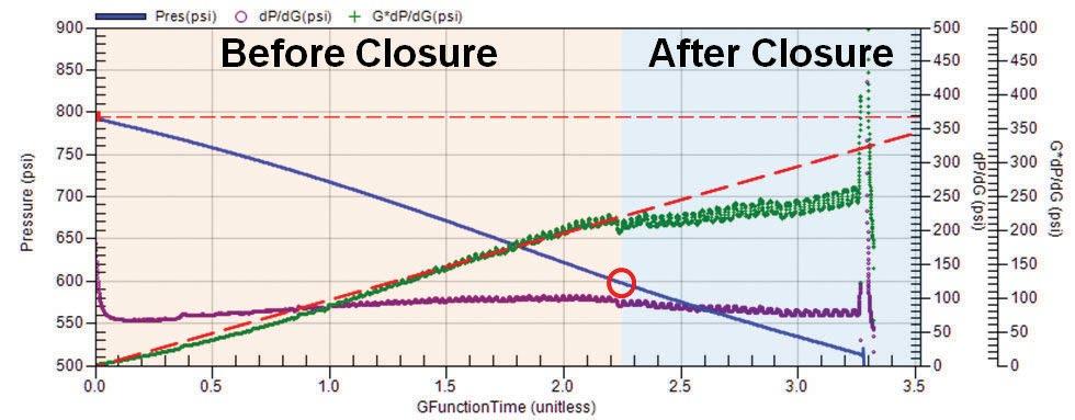
Fig. 2 displays the pressure vs. time data acquired in the Opal CT interval. Fracture closure and re-opening pressures are highlighted on the plot, and indicate very close agreement across the injection/falloff cycles. Pressure transient data was analyzed in real-time (Fig. 3) to identify changes in the flow regime as the fracture closes. There is a change in slope of the G-function derivative when the fracture closes, and the highlighted red circle shows the corresponding closure pressure. Since the closure pressure from the first and second cycles were consistently repeatable, the third cycle was used to confirm reopening pressure. Test duration in Opal CT was 127 minutes. Three successful tests were performed in the Opal CT interval, and four successful tests were performed in the Quartz interval.

Fig. 1 - Microfracture Test Performed in the Quartz Interval

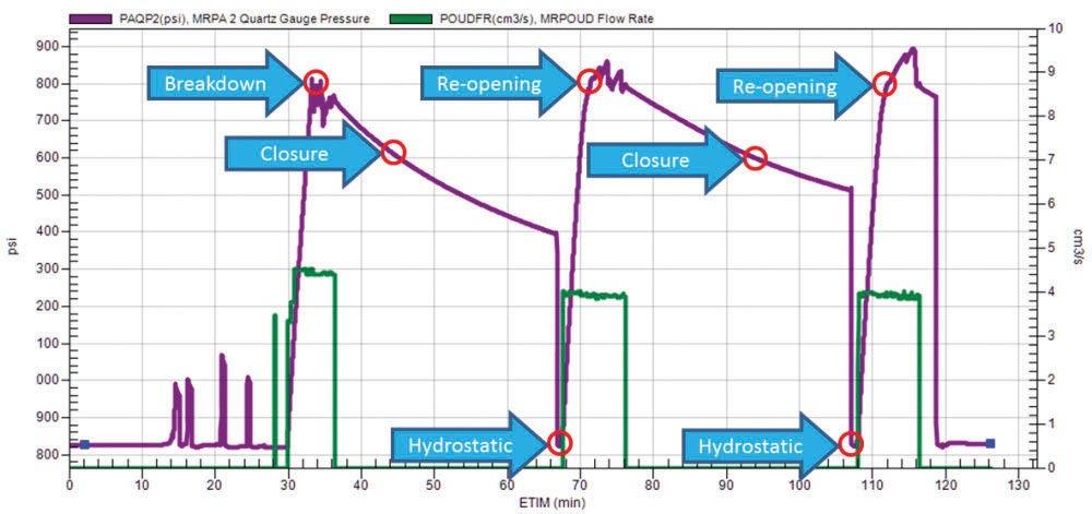
Fig. 2 - Microfracture Test Performed in the Opal CT Interval

Calibration of Stress Profile with LOT / FIT Results The Leak-off Test (LOT) and Formation Integrity Test (FIT) data for Well 1 were plotted on a pressure vs. depth chart along with the data from offset wells. Microfracture data from Well 1 was used to calculate closure stress, and results were plotted to compare with LOT and FIT data (Fig. 4). Pore pressure was estimated from the pressure/temperature surveys in off

set wells before the Antelope Shale wells were drilled. A FIT was run at each casing shoe to estimate the fracture gradient and identify the available window for mud weight. It was desired to keep the mud weight above pore pressure but less than fracture pressure. The mud weight range to drill Well 1 was 9.8 – 10.5 ppg. In essence, both the FIT and LOT refer to formation strength, except that FIT pressures did not actually break the formations, while LOT pressures did break the formation.

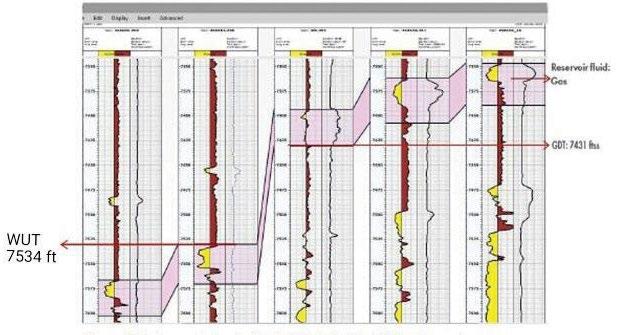
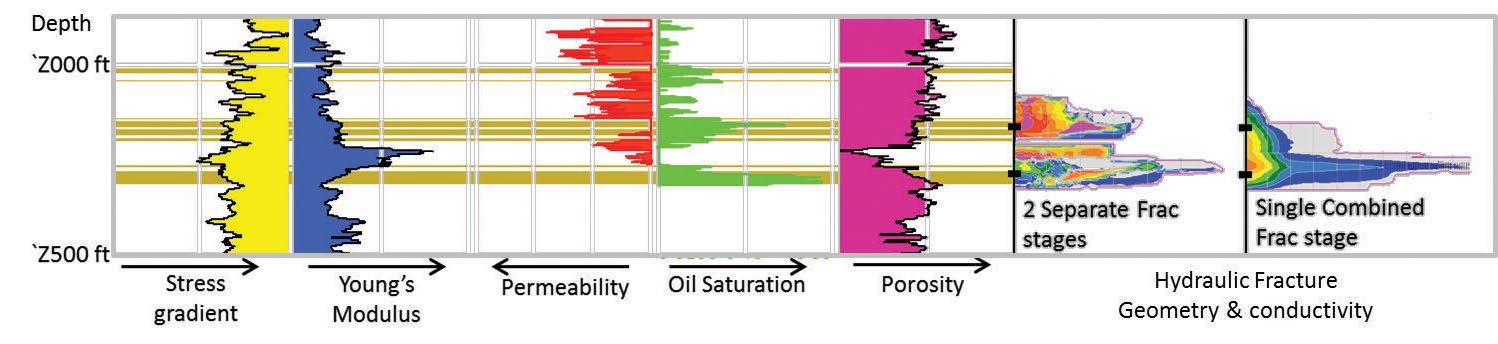
Application of Stress Profiling (Number of Fracture Stages Optimization) Multiple pay zone intervals in Well 1 were selected on basis of rock properties (e.g., porosity, oil saturation and permeability). Calibrated and corrected vertical stress profile across the pay interval was used in 3D fracture simulator to identify potential fracture boundary and optimum number of stages, to stimulate all pay zone intervals effectively (Fig. 5). Different combinations of fracture pumping schedule, proppant quantity, fracturing fluid type, and pump rate were modeled with 3D fracture simulator to better define the fracture growth and identify fracture boundaries. The optimized 3 fracture stages across Quartz phase and 4 stages across Opal CT phase effectively cover pay zones with good proppant placement at the end of fracture closure (Fig. 5). Simulation also assured that fracture would not communicate with the water wet formation on top of Quartz.

Perforation and Fracture Placement Optimization Perforation placement and fracture initiation depth for an individual fracture stage is critical to achieve effective wellbore connectivity, after proppant settling in shale formation. Various low stress sections were identified to select the preferred location for maximum fracture conductivity across perforation, which will result in good wellbore connectivity. The perforation strategy of single vs. multiple clusters was evaluated for each fracture stage (Fig. 6). Fracture growth resulting from the 3D fracture simulator indicated that in Opal CT, single cluster is the preferred option to achieve longer fracture half-length and confined propped fracture, which improves connectivity at the perforations. However, in the multiple cluster scenarios, the fracture had the tendency to grow upwards from top perforations, achieving longer fracture height but less fracture half length.

In Quartz phase, two options to achieve effective stimulation coverage were evaluated with 3D fracture simulation. Stress profiling was very critical in this scenario, as the deeper pay zone had low stress gradient. In the case of single large size fracture stage across multiple pay zones, the 3D fracture simulation results show that fracture grows preferentially in the lower pay zone, thereby the upper pay zone stays understimulated. By comparison, in the individual small size fracture stage, both upper and lower pay zones were optimally stimulated, as fractures achieve longer propped length and good wellbore connectivity with high proppant placement at perforations (Fig. 7). Thus, individual small fracture stages were selected as the preferred stimulation option.

Fig. 4 - Cross Plot of Pressure vs. Depth

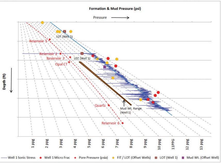
Fig. 5 - Selection of Pay Zone on Well 1 and Identification of Fracture Boundary to Determine Optimum Number of Fracture Stages

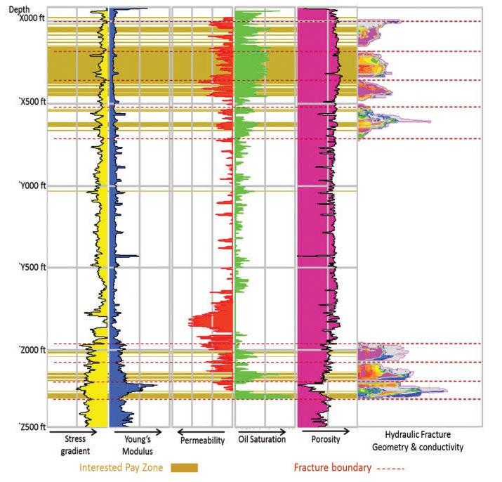
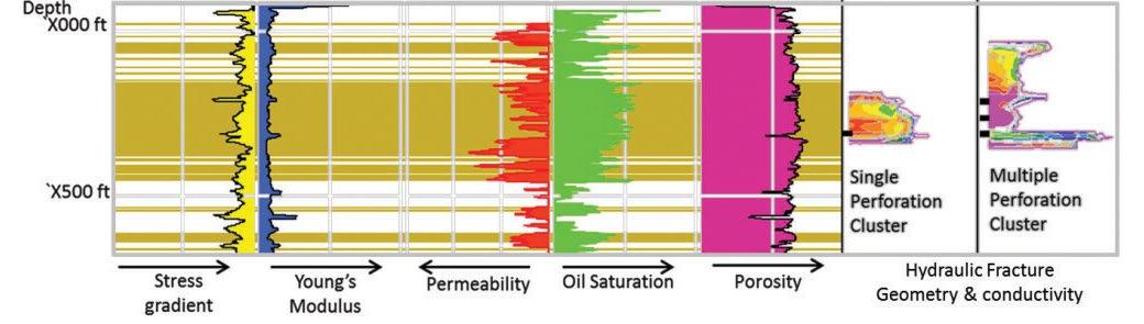
Fig. 6 - Comparison of Perforation Cluster Option (Single Cluster VS Multiple Cluster) and Impact on Fracture Growth and Proppant Placement

Mud Weight Adjustment The well was drilled with 9.8 - 10.5 ppg mud, which was selected on the basis of LOT/FIT and predicted pore pressure data. It was desired to keep the equivalent mud weight below the fracture pressure to minimize fluid loss due to formation. The calibrated stress profile from Well 1 along the drilled depth helped decide a reliable mud weight range for different sections of the wellbore (Fig. 4). This was further useful in narrowing down the mud weight range while drilling subsequent wells.

Integrated Model Studies

Kelly Edwards - Reservoir Engineering Advisor, Korean National Oil Corporation, Canada

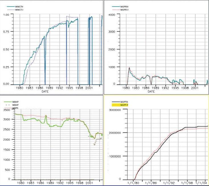
What is an Integrated Model Study? An integrated model study is a reservoir simulation study carried out using all available data from all sources and disciplines that relate to the reservoir. Data comes not only from the engineering realm, but may also come from geologists, geophysicists, and petrophysicists. Simulation modes are generally full-field models used to model the geology, and cover the full history of the reservoir. They can range in size from small models with few wells and little production data, to models of giant reservoirs with billions of barrels of oil, hundreds of wells, and immense amounts of production, completion and pressure data. Data requirements for large models can reach tens or hundreds of millions of numbers. When building an integrated model, data from different disciand gas rates, and model pressures match measured pressures, we can achieve a good history match. If the match is poor, adjustments are made to the input parameters to drive the model towards a better match. History matching is an important process because it increases confidence in the predictive capabilities of the model. History matching can also highlight deficiencies or errors in the input data, as well as provide valuable insight into reservoir characterization.

What Data Goes into Integrated Models? Any, or all, of the following data types can be incorporated into a typical integrated model. This list is not exhaustive, but covers the most common types.

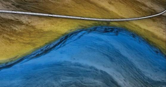
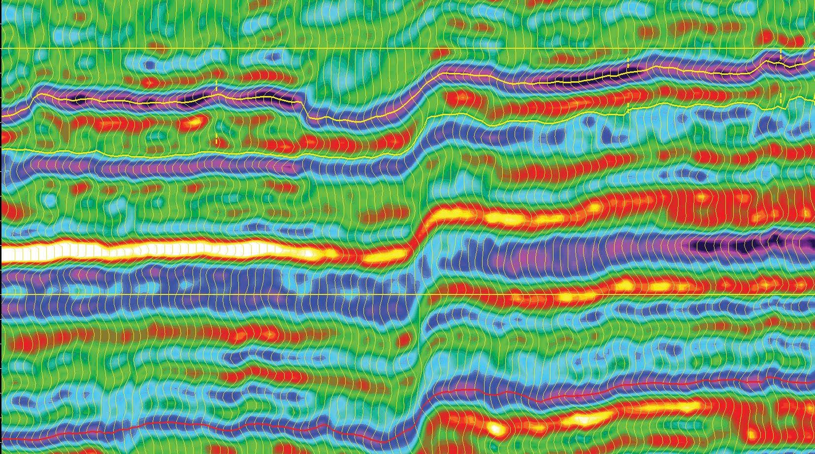
Fig. 1 - Seismic Section Showing Top and Base of Reservoir Zone (Faint Yellow Lines), and a Fault (in the Middle of the Section)

plines, measured at immensely different scales, must be integrated. This is not an easy process, and specialized software is necessary. Prior to building the model, much time and effort goes into data collection and quality control. The collection and QC of data can consume a substantial portion of study time. Geological Model – Geologists formulate a model of processes that created the reservoirs. These models are usually conceptual, and, at some point during the study, must be transformed

What are Integrated Models Used for? Integrated full-field models can be created at any time during the reservoir life cycle. Early in the life cycle, there is little data, and models can be used to evaluate uncertainty in OOIP, reserves, and production rates. In addition, it can be used to determine an optimum development plan in the light of uncertainties. As the reservoir becomes more developed, more data goes into the models, but questions to be answered by the models become typically harder to answer. Later in the reservoir life cycle, models can be used to evaluate infill locations, field development scenarios, or predict incremental recovery for a change in process (e.g., waterflooding a reservoir on primary production, or converting a waterflood to an EOR process). An integrated model must be validated before it can be used to make predictions. This is done through the process of history matching, where changes are made to the model inputs so that production rates from each well in the model match actual production rates. When each well shows a good match on oil, water

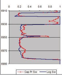
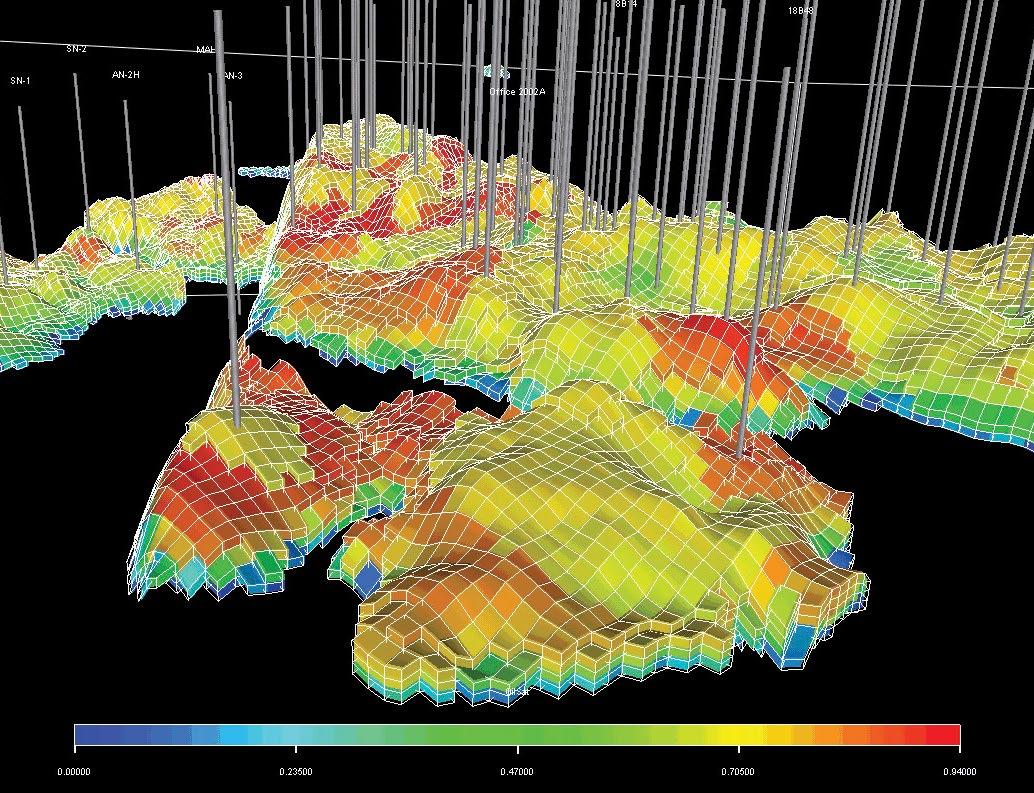
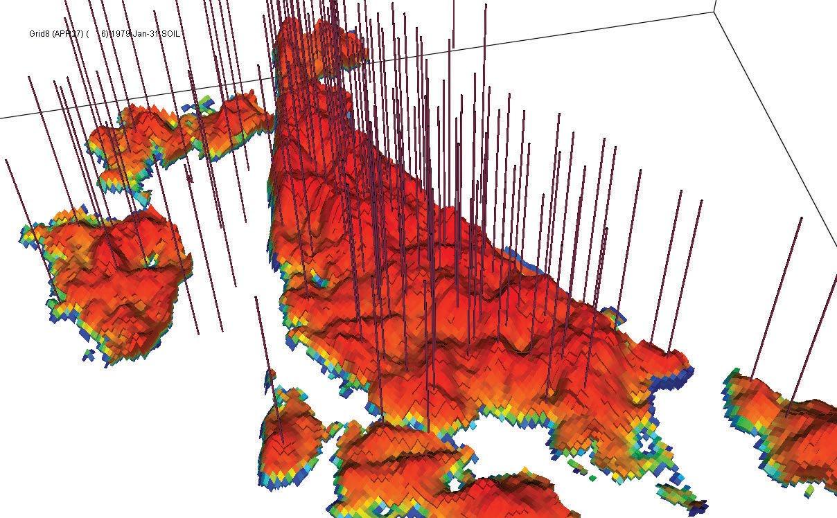
Fig. 3 - An Integrated Model Showing a Number of Individual Oil Pools and Well Locations. All Pools Sit on an Aquifer, Which Is Not Shown

into the realm of numbers to be used in the simulator. Seismic Data – Seismic information is often used to build the structural framework of the reservoir, such as the top and base, internal units, and faults. In some cases, seismic attributes can be determined, which help characterize reservoir properties or saturations within the reservoir itself. Seismic information provides detail of the interwell space, where we typically have no other data. Petrophysics – Petrophysical data is the foundation of an integrated model. Porosity and water saturations are necessary to estimate original hydrocarbon volumes. Estimates of permeability, from any source, are fundamental for estimating production rates.

be appropriately described. This data comes from PVT tests or

correlations, and includes information such as viscosity, density,

bubble point pressure, and GOR.

Production Data – Produced volumes of all fluids from every

well throughout the life of reservoir must be included. Typically,

production is reported in monthly increments. Generally, com

panies are only interested in oil or gas production, because rev

enue is derived from their sale. However, the reservoir engineer

is concerned with all fluids, whether they have value or not. For

example, injected and produced volumes of substances used in

an EOR process, such as CO 2 , must also be measured. Completion Data – Completions vary in time and space. Over

the lifetime of a well, completions can be opened, abandoned, moved to different zones, lengthened, or shortened. All these changes must be accounted for in the integrated model. Wellbore Trajectories – Wellbore trajectories are required to determine completion intervals in the model. Completions in vertical wells are easy to define. However, full wellbore trajectories are necessary to define completions in deviated and horizontal wells. Pressures – Pressures are important for material balance calculations, to estimate zonal allocations, define aquifer properties, and calculate completion skin.

Fig. 4 - An Integrated Model Showing a Number of Individual Oil Pools, and Well Locations. All Pools Sit on an Aquifer, Which Is Not Shown

Well Test Data – Well test data provides estimates of formation permeability, completion skin and distance, and orientation of reservoir boundaries. Core Data – Core data is fundamental to petrophysics, rock physics, and geological model. Rock Physics Data – Relative permeability is necessary to model multi-phase fluid flow. Capillary pressure data, which is measured in the laboratory, is required to initialize saturations. Fluid Properties – Physical properties of all reservoir fluids must