Case Study

Estimation of Oil Isothermal Compressibility

Muhammad Ali Al-Marhoun - SPE, Reservoir Technologies, Saudi Arabia

Oil compressibility plays an important role in reservoir simulation, material balance calculations, design of high-pressure surface-equipment, and interpretation of well test analysis, specifically for systems below bubble point pressure. Accurate information on the oil fluid compressibility above and below bubble point pressure is very important for reservoir evaluation.

The conventional definition of isothermal oil compressibility below bubble point pressure is being questioned on its scientific merit and challenged against the basic compressibility definition and the general trend of physical behavior of compressibility. This article presents a new derivation based on the basic compressibility definition to calculate oil compressibility below bubble point pressure. It is found that oil compressibility above and below bubble point according to the new definition is continuous and differentiable except at the original bubble point pressure cusp.

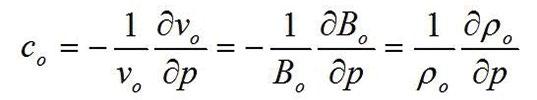
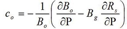
Coefficient of Isothermal Compressibility of Oil, C o By definition, single phase isothermal compressibility is de

fined as the unit change in volume with pressure. It is usually

expressed as 1/psi. This definition is valid if and only if the single

phase composition is constant. Compressibility can be calculat

ed from the slope of relative volume versus pressure of a single

phase liquid. In equation form, the point function oil compress

ibility, C o , is defined as:

(1)

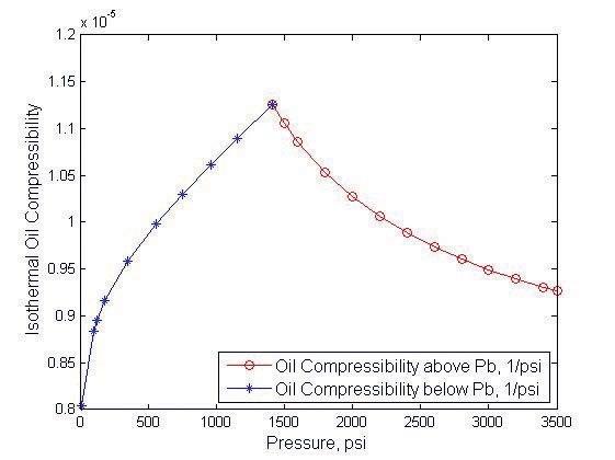
Correlations of C o above Bubble Point Typical relationship of isothermal oil compressibility, C o , with pressure above the bubble point is shown in Fig. 1.

with reduction in pressure, contrary to the behavior at pressures above the bubble point. Moreover, density of oil increases with the decrease in pressure due to the liberation of gases. Therefore, the profile of volume and density of liquid oil are opposite to the normal trends in single-phase, constant-composition fluids. A direct application of the general definition of isothermal compressibility of oil below the bubble point will lead to negative compressibility.

The typical relationship of C o according to Eq. 4 for pressures below the bubble point pressure is shown in Fig. 2.

Fig. 1 - Typical Oil Compressibility Curve above Bubble Point

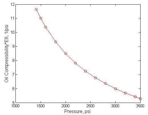
The isothermal oil compressibility factor above Bubble Point pressure can be estimated to an accuracy of 5% with:

Where; a1=-14.1042, a2=2.7314, a3=-56.0605*10-6, a4=-580.8778 (2)

ECHO • FEBRUARY 2016 Fig. 2 - Typical Oil Compressibility Curve Eq. 4 is the definition of C o below the original bubble point pressure accepted by petroleum engineers and stated in text books and petroleum technical papers as a fact. The expansion effect of gas coming out of solution expressed in Eq. 4 is wrong, because the gas formation volume factor, B g , is also changing with pressure. The gas expansion term should be:

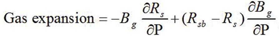
Compressibility, as stated in Eq. 1, is defined for constant composition fluids only. Below bubble point pressure, the liquid oil composition changes as pressure decreases. There is no definition of compressibility for such fluid with changing composition.

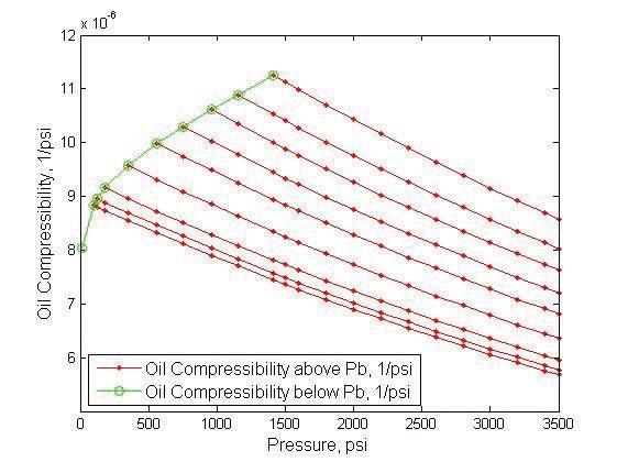
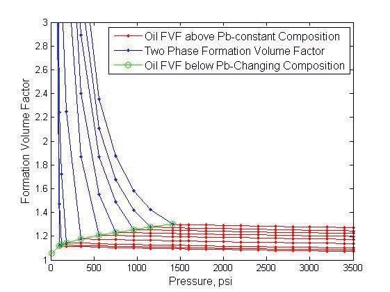
Correlations of C o below Bubble Point: Below the original bubblepoint pressure, the oil composition changes as pressure changes. Therefore, the oil compressibility, C o , below the original bubblepoint cannot be calculated as a continuous function. Fortunately, the limit of volume derivative with respect to pressure, as pressure approaches bubblepoint pressure, is defined. Since every point below the original bubblepoint is a bubblepoint for a new fluid with new composition, therefore the locus of C o below the original P b could be estimated. Eq. 1 is valid for single phase oil liquid above P b as well as below P b . The only condition required is that oil volume, density or formation volume factor and their derivatives with respect to pressure have to be taken along constant composition curve. In this case, the curve of constant composition is not clear and it is not even drawn below bubblepoint pressure. Fig. 3 shows several bubblepoints for new fluids of different composition below the original bubblepoint. Fig. 3 could be obtained experimentally if a composite liberation test is performed. Oil volume, density and formation volume factor versus pressure curves are the locus of these properties at saturation pressures for changing oil compositions. Oil compressibility at any bubblepoint pressure below the original P b is the extrapolation of C o curve of pressures above that particular saturation or bubblepoint pressure. Therefore, the locus of C o below the original bubblepoint corresponds to the locus of C o at saturation pressures corresponding to the pressure curve for the oil formation volume factor as shown in Fig. 4.

Estimation of Saturated Oil Compressibility Eq. 2 can be used for single point estimation of C o at saturation pressure with the observation of the correct evaluation of the oil relative density at the saturation pressure of interest as follows:

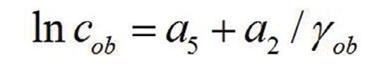
In general for any pressure, P, below original bubble point pressure, C op is estimated by:

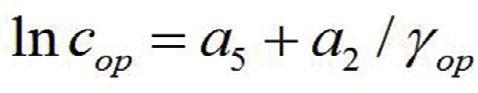
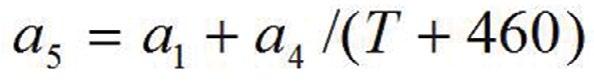
Where:

Since any point below the original bubble point is a new bubble

point for a new fluid, the term (P- P b ) in Eq. 8 is equal to zero for any pressure below the original bubble point pressure. Eq. 8 is

rewritten as:

By combining Eq. 6 and Eq. 7, C o at any pressure below the original bubble point pressure can be calculated in terms of C o at the original bubble point pressure, and live relative oil densities

at pressure of interest and the original bubble point pressure as follows:

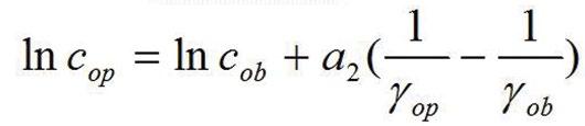
Fig. 5 clearly shows that the oil compressibility above and below bubble point according to the new definition is continuous and differentiable except at the original bubble point pressure cusp.

Fig. 3 - Locus of Bubble Point Oil Formation Volume Factor – Green Curve

Nomenclature a i = i th coefficient of equations P b = bubble point pressure, psi (kPa) B g = gas FVF , rcf/scf (m 3 /m 3 ) R s = solution gas oil ratio, scf/stb (m 3 /m 3 ) R sb = solution gas oil ratio at P b , scf/stb (m 3 /m 3 ) C = compressibility, psi -1 (kPa -1 ) C o = oil compressibility, psi -1 (kPa -1 ) C ob = oil compressibility at P b , psi -1 (kPa -1 ) C op = oil compressibility at p, psi -1 (kPa -1 ) = bubble point oil relative density(water= 1) B o = oil FVF, rb/stb (m 3 /m 3 ), B ob = oil FVF at P b , rb/stb (m 3 /m 3 ) P = pressure, psi (kPa), = oil relative density (water= 1) T = temperature, °F (K), = oil density, lbm/ft 3 (kg/m 3 ) V o = oil volume, stb (m 3 ), = oil relative density at p (water= 1) Fig. 5 - Typical Oil Compressibility Curve

Non-Radioactive Detectable Proppant First Applications in Algeria for Hydraulic Fracturing Treatments Optimization

Luca Dal Forno - ENI, SPA

Bir Rebaa Nord (BRN) and Bir Sif Fatima (BSF) fields, operated by Groupement Sonatrach-Agip (GSA, a JV between ENI and Sonatrach), are located in the Berkine basin in North-Eastern Algeria. These fields are characterized by oil-bearing sandstone reservoirs with low to medium petrophysical properties. During the development phase, to counteract the effect of pressure depletion, water and gas injections were implemented for reservoir pressure maintenance. Hydraulic fracturing has been implemented to improve well performance, both in terms of productivity and injectivity for oil producers and water injectors respectively. Hydraulic fracturing has been implemented in GSA since year 2000 to improve well performance, both in terms of productivity and injectivity for oil producers and water injectors respectively. The fracturing process has been improved over the years regarding operational procedures, enhanced reservoir knowledge, and implementation of new technologies towards resolving the many uncovered challenges. Changes to the perforation strategy, fracturing fluids formulation, rock mechanics studies, and design of proppant schedules are examples of enhancement to the fracturing practice that have been implemented recently. One of the uncharted matters in GSA, coming out from the post-job data re-processing, was the necessity of a precise characterization of the hydraulic fractures vertical coverage. The presence of several sandstone layers with different properties brought questions if the fracture had grown into an unwanted zone, or may had not properly covered the entire target formation. This article describes the successful implementation on two water injector wells of a novel non-radioactive detectable proppant for the first time in Algeria. The taggant material within the proppant has been located by comparing the pulsed neutron casedhole logs before and after hydraulic fracturing treatments. The detectable compound does not affect proppant properties, and its non-radioactive nature reduces the duration of materials delivery. Moreover, it eliminates the HSE risks linked to other tracing methods. Pulsed neutron measurements evaluation provided valuable information regarding fractures confinement, avoidance of contact with undesired layers, and possible presence of cement channeling. Furthermore, combined with sonic logs and cores data, it helped refining the geomechanical model for future interventions design in the same reservoirs. Having an accurate fracture height measurement was central to the optimization process. A number of technologies for fracture height measurement are available to the oil and gas industry nowadays, which can be broadly divided in far-field and near wellbore techniques. While microseismic and tiltmeters can be counted in the first category, temperature logs, radioactive tracers, and sonic logs methods belong to the second one. Each category has its advantages and disadvantages, making them complementary rather than competing options. Indeed, while far-field methods give a better indication of the hydraulic fracture azimuth, length and symmetry, near wellbore techniques provide more accurate height measurement, as well as proppant location.

Traceable Proppant Instead of measuring the hydraulic fracture propagation, that may or may not be propped, a near wellbore technique, indicative of where proppant had been placed, was desired. The technology selected for this project incorporates a high thermal neutron capture compound (HTNCC) at low concentrations

throughout all proppant grains in the manufacturing process. This low concentration produces no detrimental effects on any proppant physical property, including strength, and most importantly, fracture conductivity. The proppant containing HTNCC is pumped downhole and placed in the hydraulic fracture, as it is done with any standard proppant. Its detection is based on the effect that the HTNCC will have on Standard Compensated Neutron logs (CNLs) or Pulsed Neutron Capture (PNC) tools. In the case of CNL, the presence of the HTNCC will reduce the neutron count rate recorded in the detectors; while in the case of PNC, the presence of the HTNCC will reduce capture gamma ray counts and increase the computed formation capture cross sections. If run on carbon-oxygen mode, PNC logs can also determine the elemental yield of the HTNCC. Comparison of before-frac and after-frac logs in both PNC and CNT methods is straightforward, and clearly indicates the presence of HTNCC tagged proppant when other parameters are relatively constant. If the borehole environment changes be tween log runs, different tools are utilized for the two log runs, or the neutron outputs of the sources used in the before-frac and after-frac logs are different, log responses may need to be normalized utilizing logged intervals outside the fractured interval(s). It is also possible in some situations to eliminate the before-frac log entirely, if a PNC or CNT log had previously been run in the well.

Field Applications The first case study considers water injector well BRN-27. The fracure treatment was designed based on the available information from well BRN-27 and past fracturing experience in the same area. In order to assess if the upper sand layer would be affected by the hydraulic fracturing treatment, well BRN-27 was selected as candidate for implementing the non-radioactive detectable proppant. The main fracture treatment was successfully conducted, placing a total of 84 klbs in formation at a maximum concentration of 7.4 ppg. Following the treatment flowback, the well was logged with a PNC tool for the traceable proppant placement interpretation. Formation sigma and captured gamma ray, which count rate measurements for both pre and post fracture conditions, were compared and analyzed for tagged proppant identification. The strong attenuation of neutron counts and increase in formation

Fig. 1

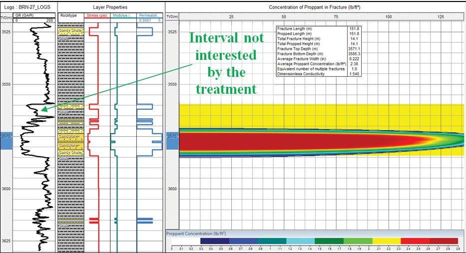
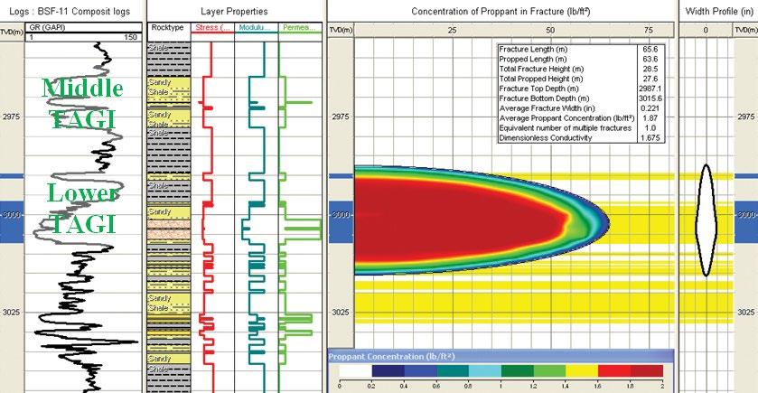
sigma between the pre and post fracture logs suggest a wide fracture. From the interpretation, it was also evidenced that the fracture propagated in a very confined mode within the boundaries of the perforated sand body. The actual fracture height of 13 m derived from the tagged proppant interpretation was then considered as a fixed input to the fracture model for net pressure matching. In order to satisfy the measured fracture height, closure stress and Young’s Modulus of the shale thin layers above the perforated interval were considerably increased, compared to the values used in the design phase. As it can be observed in (Fig. 1), the resulting geometry is extremely confined within the main interval, not contacting the upper sand layer with poorer petrophysical properties. The second case history is dedicated to well BSF-11, drilled in 2013 as a water injector in the Lower TAGI formation. The main objective of this well was to provide pressure support to the close oil producer, open in the same interval. Since BSF-11 was the only injector in the field specifically dedicated to this target formation, it was extremely important for the hydraulic fracturing treatment to remain confined within that interval. For this reason, non-radioactive detectable proppant was selected for this well. The main fracturing treatment was performed placing a total of 55 klbs of traceable proppant in formation, at a maximum concentration of 7.5 ppg. Tip screen-out occurred shortly before the designed end of the job, creating an extremely compacted proppant pack, and therefore increasing the final fracture conductivity. Once the underflushed proppant in the wellbore was cleaned up and all the treating fluids were flowed back, a second run of PNC log was performed on the same interval of the pre fracture run. Pre and post fracture PNC curves were compared and analyzed, in order to assess the placement of the non-radioactive proppant within the formation. Clear proppant signals were detected in the interval from 2984 to 3010 mMD. After-fracture near and far detector count rate logs decrease, and the after-fracture formation sigma log increases simultaneously, suggesting the presence of a wide and deep fracture. From 3010 to 3015 mMD, the after-fracture near count log decreases but the after-fracture formation sigma log hardly changes. This suggests that in this interval, some tagged proppant might be only present in a near-wellbore region, such as cement annulus. Therefore, the actual fracture height can be interpreted at around 26 m, extending from 2984 to 3010 mMD. With the accurate height measurement, the fracture model was re-calibrated to match the actual created geometry (Fig. 2). The upper shale layer closure stress was slightly increased in order to satisfy the actual propped height. The Middle TAGI formation was not contacted by the stimulation, confirming the achievement of the primary treatment.