Technical Manual for the Use of Software
in the Works of Roger Reynolds

Technical Manual for the Use of Software
in the Works of Roger Reynolds
Roger Reynolds with Jaime Oliver
and Paul Hembree
As used in:
SEASONS: Cycle 1, Dream Mirror, MARKed MUSIC, Toward Another World, Positings , george WASHINGTON, and FLiGHT
A member of the EDITION
The technological environment used in Roger Reynolds’s works involving real-time, interactive computer performance
This document describes the algorithms and performance strategies of the live electronics developed for Roger Reynolds’s SEASONS project, and subsequently used in other works including Dream Mirror, MARKed MUSIC, Toward Another World, Positings, george WASHINGTON, and FLiGHT The algorithms presented here were conceived by Reynolds and developed in collaboration with several programmers. Pei Xiang did an initial version of the SMEARZ algorithm. Ian Saxton programmed the PROLIF, SMEARZ, and MATRIX algorithms in Pd while involved in the realization of Reynolds’s multiple-percussion work Sanctuary. The further development of these algorithms and their specific application in SEASONS was accomplished by Jaime E. Oliver La Rosa, including their adaptation for live performance with a controller (also in Miller Puckette’s Pd) and the development of the THINNR algorithm. Paul Hembree has continued work optimizing the algorithms and adjusting their spatialization strategies. This document represents the current state of the software (November, 2014), and conceptual approaches to performance with a computer. Development is ongoing.
These algorithms were at first thought of as processes with relatively pre-determined trajectories. PROLIF offered a gradual proliferation from a singular source sample towards a wide diversity of flocking transformations (the process is reversible); SMEARZ proposed a radical temporal expansion and blurring of its source material while retaining the source’s morphology; MATRIX offered arbitrarily complex rhythmic patterns based on a temporal fracturing and patterned replication of source material, also manifesting the original morphology of the source sample, though temporally expanded. THINNR was conceived from the start as a real time algorithm that allows for radical temporal expansion and formant-like filtering carried on by two simultaneously and independently evolving processes.
A principal goal of the electronics in Reynolds’s work has been to incorporate the computer musician as a performer and therefore, as member of an ensemble. Although, in the original algorithms, the variable nature of several internal processes offered change from realization to realization, there was little opportunity for dynamically controlled alterations during performance. In the current versions, we have chosen several parameters for each algorithm that are subjected to live control. Combinations of available parameters, in turn, provide the computer musician performer with the ability to start, stop and change processes dynamically in interactive response to other members of an ensemble.
Reynolds’s scores for works that utilize this technological environment have two categories of annotation relevant to computer events: SAMPLES to be recorded and CUES to be performed.
SAMPLES are numbered in the order they occur in the score. They may entail one or several instruments at the same time.
The preferred strategy is to pre-record the SAMPLES rather than to capture them live in performance. This allows for high quality SAMPLES recorded with several microphones to improve timbral subtlety, as well as to reduce noise and obtain optimal expressive character. One can choose a recording with a desired instrumental or harmonic balance, or edit to create a preferred amount of silence at the ends of a sound file
Most crucially, since the algorithms are based on prepared SAMPLES, changing them in each performance would literally change the “computer instrument” for a CUE. Often a specific trait of a particular sample recording becomes a key element in the CUE, which is explored in rehearsal and performance.
In some cases, a CUE might ask for switching between source samples. This is accomplished by preediting the source file, and placing the desired samples in proper succession. In this way, as will become clear throughout this document, a SMEARZ event might navigate three samples in succession or a MATRIX event might switch very quickly between different samples.
CUES in Reynolds’ scores are the actual performance events. They always specify two things: (1) the source SAMPLE to be used and (2) the algorithm with which it will be processed.
All CUES have start- and end-points. Starts and stops are executed using separate buttons on a CONTROLLER.
When a CUE is launched, the samples and algorithms are called, the latter with a set of predefined values for each algorithm variable. These values are provided to the computer performer in a “technical score” as a point of departure for each CUE.
The score also contains graphical and textual notations for each CUE. These are intended as general indications about the trajectory of parametric variation after launch and following on from the preset departure values. The graphic indications are general enough to provide the performer with a certain degree of liberty as to how they are to be realized.
A primary objective for the use of computer algorithmic processing in performance is to achieve a sense of performed subtlety and interaction: allowing the computer performer to be able to adapt to and shape processes in real time with the acoustic performers. To this end, we sought a controller that was readily available and expressive enough.
For SEASONS, a motorized multi-slider controller with at least 8 sliders is required. A Diagram of the BCF2000 interface by Behringer is shown in Fig. 1.
It is important that the sliders are motorized because at each CUE launch they must rapidly reposition to precise pre-defined initial values. CUES are launched with button B7a and stopped with button B7b. In some cases, the computer performer can choose to have additional reset points within a CUE. These are termed PRESETS. PRESETS 1, 2, 3 and 4 are launched by buttons B1a, B1b, B1c and B1d, respectively. Other buttons can be used if more PRESETS are needed.
It is valuable that this controller’s 8 sliders can be reasonably controlled by two hands. To make the task yet more optimal, our mapping strategy places the sliders (the parameters) that require greater mobility at the sides (i.e., at sliders 1 and 8).
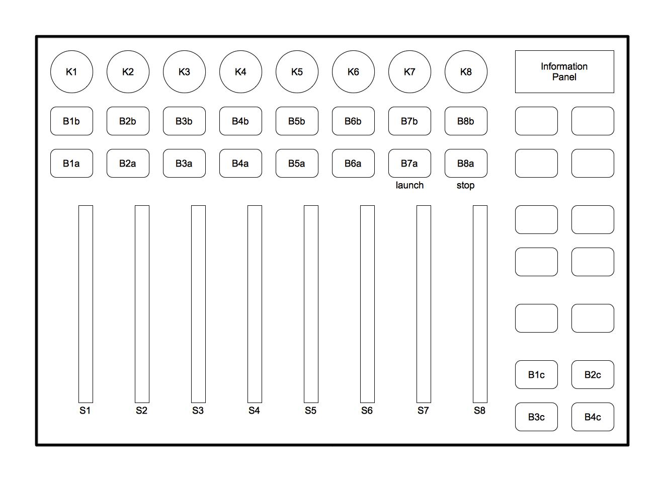
Fig. 1. Diagram of the BCF2000. Sliders are labeled S, buttons B and knobs K.
PROLIF
General Description:
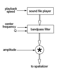
In PROLIF, a (usually) brief seed sound file, or several such sources are used as models for massive replication in a number of varied forms; altered loudness, transposition, and spectral filtering. Each replicated file derives from its seed but is distinct. Because the densities in PROLIF can become very great, it is important that the replicants become spectrally thinner and spatially distinct so as not to mask one another. The PROLIF algorithm uses a 96-voice polyphonic sample player. Each voice consists of a sound file player, a bandpass filter and an amplitude control as seen in Fig. 2.
Each voice has three possible modifications: Transposition, Filtering, and Amplitude.
• Increasing or decreasing the original file’s playback speed transposes its pitch. If the file is played slower, the duration increases and the perceived pitch lowers, and vice versa. This dimension is controlled by two parameters: PITCH and PITCH RANGE.
• Filtering is controlled by two parameters: Q and CENTER FREQUENCY.
• Amplitude is controlled by two parameters: MINIMUM GAIN and GAIN RANGE.
A global automation controls which voices are played and with what parameter values. The control parameter for this global automation is DENSITY, a random process that controls the number of elements per unit time in relation to a norm. Each time a voice is instantiated, values from each of the voice parameters are polled. The polled parameter values can either be directly fed to control dimensions of the algorithm or they can be construed as minimum and maximum values constraining a random process. Such random processes have a normal distribution. For example, when a voice is instantiated and the parameters PITCH = 8 and PITCH RANGE = 6 result from a polling, the final transposition will be between 8 and 14 semitones. The result of this process can be seen in Fig. 3.
Amplitude control behaves in a similar manner: local voice gain = MINIMUM GAIN + GAIN RANGE.
The CENTER FREQUENCY of the filter varies randomly across the audible spectrum. Given this, Q determines the extent of the filter’s impact on the PROLIF process. Q is the steepness of the filter and varies from 0 (flat, all-pass) to 100 (steep and narrow filter).
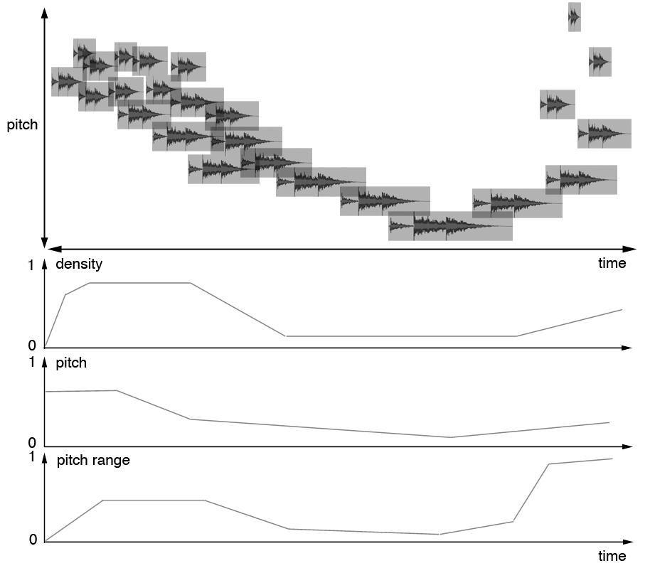
Fig. 3. Evolution of a PROLIF event showing the effect of DENSITY and the combination of PITCH and PITCH RANGE.
Additionally, the PITCH RANGE of PROLIF is divided into three layers, low, medium and high (shaded dark, medium and light in Fig. 4, top), assigned to three different outputs. As might be assumed, the lowest pitched third of PROLIF voices are assigned to the low layer, the middle pitched third to the medium layer, and the highest pitched third to the high layer. In the special case when PITCH RANGE = 0, when there is no transposition, PROLIF voices are then randomly distributed to the three layers in order to generate sound in all three outputs, even if those outputs end up carrying identically pitched material.
These three layers are then reverberated and spatialized differently using the ARC or FLOCK SPAT strategies. The low layer is typically dry, moves slower, and is confined to a space near the listener, while the medium layer is slightly wetter, moves faster, and can move further away, while the highest layer is very wet, moves extremely fast, and has a very large spatial range (see bottom of Fig. 4). The MIGRATION RATE parameter controls speed and character of the spatialization, while the REVERB parameter scales all reverberation proportionally. Different spatialization and reverberation greatly aids in the perceptual salience of the three PROLIF layers. See the SPATIALIZATION section for details.
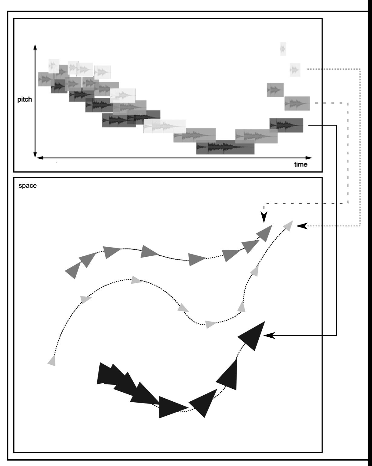
Fig. 4. Relationship of PROLIF pitch layers to spatialization speed and character in FLOCK SPAT. Top: three pitch layers, with dark, medium and light shading corresponding with low, medium and high pitches, as they are assigned to slow, medium and fast spatial trajectories. See the SPATIALIZATION section for more information on trajectories like this.
Performance:
Each PROLIF event has two discrete (on/off) controls: LAUNCH and STOP. When the STOP button is pressed, the sliders stop controlling their respective parameters and the voices that are continuing to play do so in the same fashion until their processes are finished.
The event has a set of parameters, which are grouped in fixed and variable categories. Fixed parameters are pre-set for each CUE. Variable parameters are given initialized values for each CUE, but can be modified during performance through the use of the CONTROLLER. Parameters can vary either as a single graduated value or as a pair of minimum and maximum values that define a range within which random values are chosen. These are notated below, respectively, as val or rand.
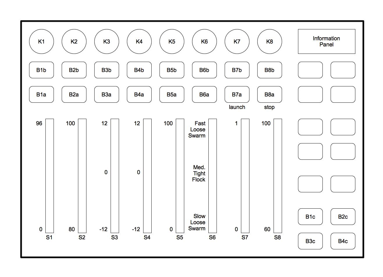
Fig. 5. Assignment of variables to the controller with minimum and maximum values for each slider. S1 = DENSITY (number of voices), S2 = GAIN RANGE (dB), S3 = PITCH (measured in half-steps), S4 = PITCH RANGE (measured in half-steps), S5 = Q, S6 = MIGRATION RATE (cf. SPATIZATION below), S7 = REVERB (wet:dry ratio), S8 = GLOBAL AMPLITUDE (dB)
Visual Feedback:
There are several sources of visual feedback to the computer musician during performance: (1) the momentary map of all slider positions, (2) the information panel at the top right of the CONTROLLER, which shows the current MIDI value of an active slider, (3) additionally, the current number of voices is shown in the graphical interface (GUI) of the current algorithm on the computer screen. This allows one to know if the voice allocation is optimal. It is always the case with these algorithms that one needs to rely mainly on listening.
Fixed Parameters: MINIMUM GAIN (val), CENTER FREQUENCY (rand)
Variable Parameters: DENSITY (val), GAIN RANGE (rand), PITCH (val), PITCH RANGE (rand), Q (rand), GLOBAL AMPLITUDE (val).
Variable Parameters are distributed as seen in Fig. 5
S1: DENSITY
This slider controls the aggregate density of the output throughout the duration of a PROLIF process. It involves a certain latency but can produce an organically varied impression if altered during the course of the process.
A total of 96 “voices” is available. The number of seed files equally divides the distribution of this resource; for example, if the event uses two seeds, each of them will have a maximum of 48 voices. Thus, if multiple seeds are used, the potential density of each PROLIF component process is attenuated.
Since the minimum value for this parameter is zero, bringing this parameter to zero, constitutes the most perceptually elegant way of exiting a cue (rather than relying upon GAIN).
S2: GAIN RANGE
Local voice gain is determined jointly by MINIMUM GAIN + GAIN RANGE.
The value of MINIMUM GAIN is pre-established for each CUE (default = 80 dB). This slider controls GAIN RANGE (default range = 20 dB). Therefore, if the slider is at the top, that is, at 100 dB, the resulting gain will be normally distributed at 90 ± 10 dB
S3: PITCH
Pitch Transposition = PITCH + PITCH RANGE.
This slider determines a reference pitch transposition. When used alone (PITCH RANGE = 0) it transposes all instances of seed replication. So for example, PITCH = 12, will transpose all instances of seed replication one octave higher than the seed’s original pitch.
This parameter can be active in a positive or negative direction. The slider center is 0. (default min = -12, max = +12 half-steps)
S4: PITCH RANGE
This slider determines a range of deviation from PITCH. It constrains the transposition of all instances of seed replication according to a normal distribution around the value of PITCH. So, if PITCH = 2 and PITCH RANGE = 12, the resulting transpositions will range between -4 and 8 half-steps: 12 / 2 half-steps above and below the center value of 2 (2 ± 6 half-steps)
This parameter can be positive or negative. The slider center is 0. (default min. = -12, default max. = +12 half-steps). The range of its output is divided into three layers: low, medium, and high. These layers are reverberated and spatialized differently (see below).
S5: Q
Given that CENTER FREQUENCY is set randomly within pre-established boundaries as a Fixed Variable, the steepness of Q determines the filter’s impact on the algorithmic output. Again, Q varies from 0 (all-pass) to 100 (steep, narrow filter).
The objectives of this parameter are to thin spectral density and increase the timbral diversity of the aggregate result. However, if the aggregate result’s spectral energy is not rich enough, it can cause a perceived loss of intensity that must be compensated for.
This compensation can be achieved by increasing DENSITY to increase the amount of material being processed, by increasing PITCH RANGE to increase the frequency range subjected to filtering, or by increasing GLOBAL AMPLITUDE or AMPLITUDE RANGE.
In the ARC-TRIAD strategy, the MIGRATION RATE controls the transition time between successive speaker locations and this in turn influences the sense of continuity of the spatialization over time. In the FLOCK-SPAT strategy, MIGRATION RATE determines both the speed and character of spatial movement using a flocking simulation. Each of the three layers of the PROLIF output are spatialized differently, with the lowest layer moving slower in a confined space, the middle layer moving faster in a larger space, and the highest layer moving very fast in a very large space. See the SPATIALIZATION section below for the strategies used for the various algorithms, and further details on how multiple FLOCK SPAT behaviors are controlled by the MIGRATION RATE fader.
This slider increases the ratio of reverberated (wet) to un-reverberated (dry) signal applied to the output of PROLIF Reverberation is applied proportionally to the three PROLIF layers, with the lowest layer receiving very little, the middle layer receiving a medium amount, and the highest layer receiving the most reverb. The actual amounts are scaled by this parameter. Reverberation is incorporated into the FLOCK SPAT strategy as a depth cue; thus, the MIGRATION RATE and REVERB parameters are interdependent. For example, turning down REVERB would reduce the perception of spatial distance, while turning down MIGRATION RATE could freeze sounds in positions that generate very little reverberation.
This is a separate control from the local gain of each replicant. It controls the aggregate impact of the algorithmic output.
Note, again, that, when a fade out is desired, it is more elegant to use DENSITY than GLOBAL AMPLITUDE.
SMEARZ
General Description:
SMEARZ processes sonic gestures so as to blur their definition and to spread their shapes out over time. If one imagines drawing a moistened thumb forcibly across a word written on paper with pencil, the intent becomes clear: the basic identity of the shape remains detectable, but its content, its “implications” are spread out in space.
The SMEARZ algorithm involves three separable stages, analysis, construction of an “event map”, and “navigation” of this map.
The SMEARZ algorithm begins with a seed that is analyzed with an onset detector to determine the location of each significant amplitude peak in the file (Fig. 6). Thresholds for the onset detector are adjusted according to the nature of the source material, e.g., percussion (noisy) events have higher thresholds because of the relative strength of their transients.
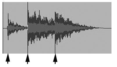
6. Onset Detection in seed file
A linear amplitude envelope is applied to the area around each detected onset peak. The length of the base of this triangular envelope is a parameter called SKIRT. SKIRT refers to the temporal spread (in msec.) around the detected peak. This generates a virtual “sub-file” for each onset as seen in Fig. 7.
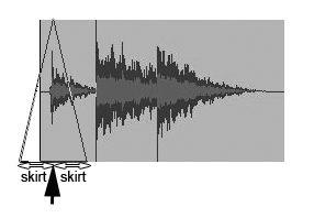
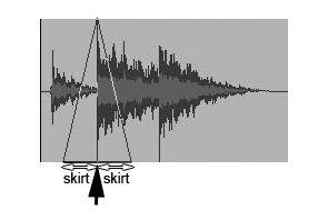
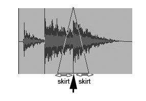
Fig. 7. Amplitude enveloping around each onset.
An FFT analysis is then performed on each sub-file to obtain a magnitude spectrum. This spectrum is separated into three sub-spectra: g1, g2 and g3 obtained by distributing frequency bins according to a parameter called BIN DISTRIBUTION.
So for example, if BIN DISTRIBUTION = 4, bins 1 - 4 will go to g1, 5 – 8 to g2, 9 - 12 to g3, 13 - 16 to g1, and so on, forming interlocking sets of spectra. The number of bins is equal to the window size, which is normally 2048 in the current version of the patch. The minimum BIN DISTRIBUTION is 1, with every third bin assigned to a sub-spectrum, and the maximum is one-third of all 2048 available bins, or about 683 bins assigned to each sub-spectrum This process can be seen in Fig. 8 where BIN DISTRIBUTION = 4.
This distribution determines the “grain” of the sub grouping. The nature of the grain, in turn, influences the goal of balancing the energy between the three sub-groupings and also determines their perceptual distinctiveness from one another. As one would imagine, g1 might be noticeably “darker” than g3.
Furthermore, the depth of differentiation between sub-spectra may be altered using the INTERLEAVE DEPTH parameter. When INTERLEAVE DEPTH is 0, the spectral energy is identical in each subspectrum, and is divided into thirds, one-third for each sub-spectrum (Fig. 8, left), making them spectrally and timbrally undifferentiated. They continue to be divided into three layers for stretching purposes (see below) When INTERLEAVE DEPTH is 1, bins are exclusive to each sub-spectrum, thus creating maximum spectral and timbral differentiation (see Fig. 8, right) A linear cross-fade is applied between these two states, creating the potential for partially interleaved spectra (Fig. 8, middle).
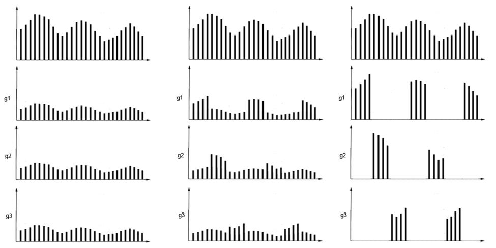
Fig. 8 Top row: original spectrum is presented for each column. Bottom three rows: Three sets of spectra, g1, g2 and g3 for BIN DISTRIBUTION = 4. Left column: INTERLEAVE DEPTH = 0, Middle column: INTERLEAVE DEPTH = 0.5, Right column: INTERLEAVE DEPTH = 1.
Each of the three subspectra is independently stretched around the detected onset point according to a parameter called STRETCH FACTOR. The STRETCH FACTOR measures the proportion of stretching with respect to the duration of the onset point material in the seed file. This factor is added to each subspectrum. So, if the seed were 100 msec, and the STRETCH FACTOR 0.5, g1 would be 150 msec, g2 200 msec and g3 250 msec. This generates a new mapping of events that are derived from the seed file and the current values of each parameter, as can be seen in Fig. 9
This event map is “navigated” by controlling a reading point. The position of the reading point determines which sub-spectra are utilized and at what amplitude level. In the example in Fig. 9 – at that particular reading point – sub-groups g2 and g3 of the second onset and sub-groups g1, g2 and g3 of the third onset will be heard.
The reading point’s continuous relocation is controlled by a parameter called READING RATE, which controls automated reading (beginning from the initial position of the reading point), such that when READING RATE = 100%, the detected onsets retain the timings of the original seed file. When the rate is 50%, their spacing out over time is proportionally doubled.
When, in A Mind of Winter (the fourth movement in SEASONS: Cycle I), a SMEARZ-processed sound is “frozen”, READING RATE = 0 and therefore the reading point is static, the SKIRT and STRETCH FACTOR can nevertheless be dynamically changed to transform the event map. Change in the output is thus created without moving the READING POINT.
On the other hand if both SKIRT and STRETCH FACTOR are static, the event map is also static, only obtaining change through the movement of the reading point. Both the event map and reading point can change dynamically at the same time.
Finally, the event data resulting from a given reading point are fed to a bank of phase vocoders so as to accomplish the desired differential stretches dictated by STRETCH FACTOR, and each sub-spectrum is spatialized independently. The number of phase vocoders in this bank is constrained by CPU limitations, but the minimum necessary for fidelity has been found to be sixteen.
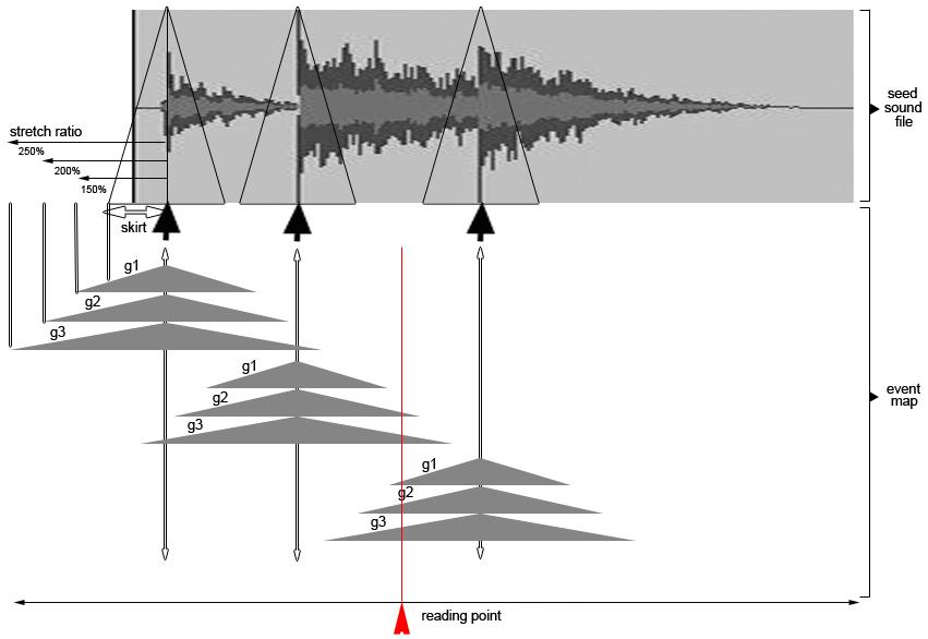
Fig. 9. Event Map generated by SMEARZ. Reading point below, event map middle, seed file above.
The sonic density of this algorithm’s output is jointly determined by a combination of: the number of detected onsets (threshold sensitivity), SKIRT, and STRETCH FACTOR (spectral density). If few onsets are detected, higher SKIRT and STRETCH FACTORS will be necessary if sound continuity in the output is desirable. If, on the other hand, too many onsets are detected, SKIRT and STRETCH FACTOR must be lowered in order to avoid saturation (or not to exceed the number of available phase vocoders). The algorithm’s conceptual aim of re-presenting an original gestural entity in a time-expanded and altered condition is sometimes replaced by a process of subtle exploration of a particular facet of the originating gesture.
Performance:
Each SMEARZ event has two discrete (on/off) controls: LAUNCH and STOP. When the STOP button is pressed, the sliders stop controlling their respective parameters and the voices that are continuing to play do so in the same fashion until they are finished.
As with PROLIF, SMEARZ has a set of parameters which are grouped in fixed and variable categories. Fixed parameters are set for each CUE. Variable parameters are given initialized values, but can be modified during performance through the use of the CONTROLLER. In contrast to PROLIF, all SMEARZ parameters have singular, graduated values.
Visual Feedback:
There are several sources of visual feedback to the computer musician during performance: (1) the momentary map of all slider positions, (2) the information panel at the top right of the CONTROLLER, which shows the current MIDI value of an active slider, and (3) the current number of phase-vocoder voices and the reading position in the file are shown in the graphical interface (GUI) of the current algorithm on the computer screen. This allows one to know if the voice allocation is optimal as well as whether the end of the file is approaching.
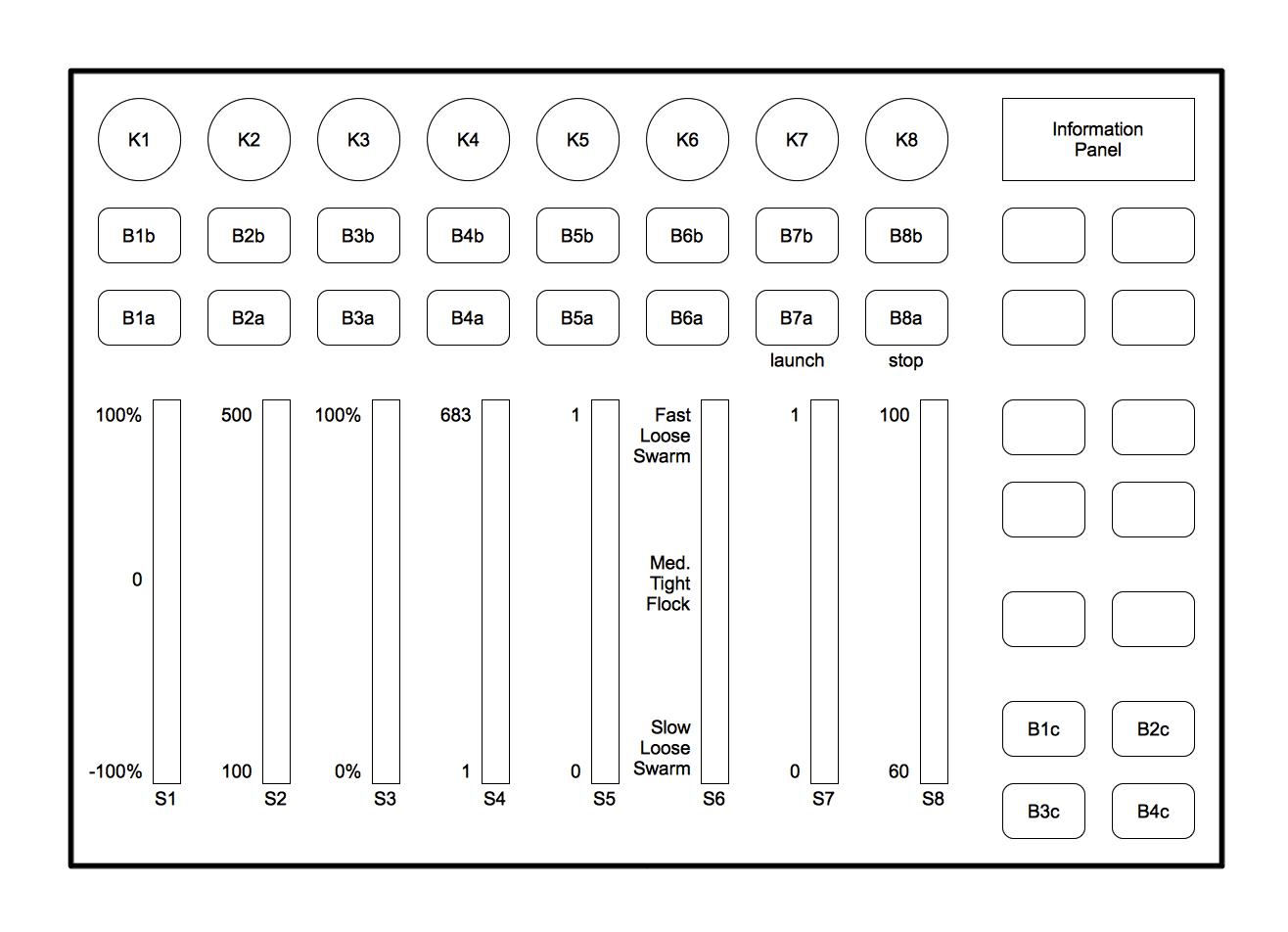
Fig. 10. Assignment of variables to the controller with minimum and maximum values for each slider. S1 = READING RATE, S2 = SKIRT (msec; max. value provided as example), S3 = STRETCH FACTOR (max. value provided as example), S4 = BIN DISTRIBUTION (bins per division), S5 = INTERLEAVE DEPTH (cf. discussion above), S6 = MIGRATION RATE (cf. SPATIALIZATION below), S7 = REVERB (wet:dry ratio), S8 = GLOBAL AMPLITUDE (dB)
Fixed Parameters: LAUNCH POINT
Variable Parameters: READING RATE, STRETCH FACTOR, SKIRT, BIN DISTRIBUTION, INTERLEAVE DEPTH, MIGRATION RATE, REVERB, GLOBAL AMPLITUDE
Variable parameters are distributed as seen above in Fig. 10.
Discussion of Slider Controlled Parameters:
S1: READING RATE
One can move the READING RATE slider in any direction at any time. 0 is at the slider’s mid-point. If the slider is set and remains unchanged, the file will be read at a constant rate from that initial point to the end (or the beginning) of the file.
• The rate at which the seed file is read can vary between the original seed file rate and 0 (a “frozen” state).
• If set between 0 (frozen) and +100%, movement is forwards in the file.
• If set between 0 and -100%, movement is backwards in the file.
The SKIRT slider must have a positive minimum, ideally no less than the window-size of the phase vocoder. The maximum value is pre-established according to the desired outcome The default minimum is 15 msec, a little more than the largest window-size normally used of 4096 samples, or 11 msec, and much more than the standard window-size of 2048 samples.
Shifting of the SKIRT from a minimum towards the maximum, results in a gradual spectral densification as this change increases the number of voices that the READING POINT might encounter in traversing the event map. Higher SKIRT values allow for lower STRETCH FACTORs and therefore, reduce undesirable sound artifacts.
Lower SKIRT values will require a higher STRETCH FACTOR if a continuous output is desired. This is due to the fact that small SKIRT values combined with a low STRETCH FACTOR, might result in spaces in the event map, so that no events are found at a given READING POINT (and therefore in silences during performance).
The minimum value is always 0 (not stretched at all) and the maximum value is pre-established according to the nature of the desired outcome. Shifting of the STRETCH FACTOR from 0 (no alteration) towards the maximum, results in a gradual spectral dispersion and variegation. This happens because each subspectrum is stretched independently and therefore, contains information from different portions of the original file such that some portions could be multiply represented and others not represented at all NB: Higher STRETCH FACTORs may produce undesirable sound artifacts, particularly if the seed file has low frequency content.
S4: BIN DISTRIBUTION
The minimum BIN DISTRIBUTION is 1, with every third bin assigned to each sub-spectra. This tightknit interleaving creates spectrally and timbrally similar (but not identical) sub-spectra. The maximum value is 683, or about one-third of all 2048 available bins with standard settings This widely spaced interleaving creates three very spectrally and timbrally different sub-spectra, each one brighter than the last. Changing the BIN DISTRIBUTION in performance can create sounds similar to those of the classic “phaser” effect, which can be useful as an expressive that is used, for instance, during the computer solos of MARKed MUSIC
S5: INTERLEAVE DEPTH
This controls the differentiation between each of the three sub-spectra. The minimum of 0 creates spectrally and timbrally undifferentiated sub-spectra that are, none-the-less, differently stretched. Be aware that this minimum essentially negates the effect of BIN DISTRIBUTION. The maximum of 1 creates maximum differentiation between sub-spectra, fully applying the effect of BIN DISTRIBUTION. INTERLEAVE DEPTH allows for another dimension of expressive potential, enabling the performer to cross-fade between dissimilar weightings and homogeneous and heterogeneous spectral complexes.
As in PROLIF, MIGRATION RATE controls both the speed and character of the spatialization of SMEARZ’s algorithmic output, using either one of two different strategies covered in the SPATIALIZATION section. Again, a three-layered approach is used to create different treatment of each of the three sub-spectra of SMEARZ, with the darkest sub-spectra moving slowly in a confined space, the middle sub-spectra moving faster in a larger space, and the brightest sub-spectra moving very fast in a very large space. See the SPATIALIZATION section below.
S7: REVERB
Further, as in PROLIF, this slider increases the ratio of reverberated (wet) to un-reverberated (dry) signal applied to this algorithm’s output The three-layered approach is applied here as well, with reverberation applied proportionally to the three SMEARZ sub-spectra, with the darkest layer receiving very little, the middle sub-spectra receiving a medium amount, and the brightest sub-spectra receiving the most reverb. See the SPATIALIZATION section below for more information on the use of reverberation as a spatial cue.
S8: GLOBAL AMPLITUDE
This parameter controls the aggregate impact of the algorithmic output. As is common with these algorithms, the use of this slider needs to be very carefully managed. When a fade out is desired it is more elegant to use the end button. When a general reduction of the amplitude of the cue is desired it is more elegant and organic to reduce the density of the algorithm by decreasing SKIRT, STRETCH FACTOR or both, rather than GLOBAL AMPLITUDE.
Also, see the SPATIALIZATION section below for the spatialization strategies used for the various algorithms.
MATRIX allows the content of a seed file to be transformed into a virtual “hall of mirrors”. A succession of progressively chosen fragments into which a sound source is subdivided is disseminated by patterned repetitions that are spatially distributed. The result produces effects that vary from timbral whir, through rhythmic insistence, towards dream-like echoing. This process is indebted to Peter Otto’s imaginative exploration of spatial phenomena.
The MATRIX algorithm involves two separable parts, analysis and execution.
The algorithm creates a “repertoire” of sound segments by establishing equally spaced starting points within the seed sound file. The file is analyzed by an onset detector, and detected onsets override the equal spacing, anticipating and replacing the next starting point with the detected onset’s location in the file. As a consequence of the override strategy (which preserves the integrity of the seed file), the segmented “vocabulary” that results will not be entirely regular in its representation of the seed file. Sound segment content is determined by starting points and the parameter SEGMENT LENGTH (in msec.).
The algorithm is executed by controlling multiple parameters of a global metronome. The basic speed of this metronome is controlled by PULSE RATE, measured in milliseconds. At each pulse of the metronome, the value of the parameter READING POINT is polled. This parameter represents a location in the original seed file. Beginning with it, six successive sound segments are selected, as seen in Fig. 11. These are then allocated to a 48-voice polyphonic player. Each voice of the polyphonic player involves a simple playback mechanism.
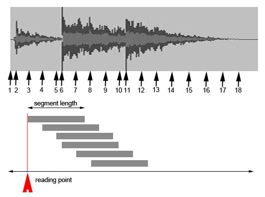
Fig. 11. Seed file segmentation (determination of segment starting points) and the selection of an initial set of 6 segments according to READING POINT and SEGMENT LENGTH.
If no adjustments are specified, all six sound segments will be heard simultaneously at each pulse, as seen in the first row of Fig. 12. labeled “normal”. However, two factors can influence this situation.
The parameter RATE DEVIATION, measured in milliseconds, is the normally distributed deviation of each pulse from its predicted timing. It allows for irregularity of pulse. This can be seen in the second row of Fig. 12. labeled “rate deviation”. The segments are still simultaneous, but the occurrence of each group of six is no longer evenly spaced in time.
The parameter JITTER, measured in milliseconds, is the normally distributed timing deviation of the selected sound segments from the pulse. This can be seen in the third row of Fig. 12. labeled “jitter”.
The dimensionality of this algorithm's output can be assessed according to the following considerations:
• The original seed sound file has a “natural” evolutionary trajectory.
• When the reading point moves in a well-connected and continuous forward direction, the integrity of this trajectory is conserved.
However, the natural trajectory can be altered according to the following influences:
• Moving the READING POINT in a radically disconnected, back-and-forth manner or, on the other hand, leaving it immobile (or virtually so).
• Very slow PULSE RATES create an echoing openness whereas extremely rapid PULSE RATE leads to timbral blur.
• The presence of reverberation can increase the blur effect while its absence promotes articulate clarity.
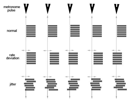
Fig. 12. Positioning of the six selected segments at a regular PULSE RATE, with RATE DEVIATION, and then with added JITTER. (Note: The number six was originally derived from the normative speaker distribution (6) considered a necessary lower limit for this algorithm.)
The variability in seed content in combination with the aforementioned considerations create a landscape of potential that is not only strikingly diverse, but also continuously navigable in an organic, performative fashion.
Performance:
Each MATRIX event has two discrete (on/off) controls: LAUNCH and STOP. When the STOP button is pressed, the sliders stop controlling their respective parameters and the voices that are continuing to play do so in the same fashion until they are finished. It also has a set of parameters, which are all in the variable category. Variable parameters are given initialized values for each CUE, but can be modified during performance through the use of the CONTROLLER. Parameters can vary either as a single graduated value or as a pair of minimum and maximum values that define a range within which random values are chosen. These are notated below as val or rand.
Visual Feedback:
There are several sources of visual feedback during performance: (1) the momentary map of all slider positions, (2) the information panel at the top right of the CONTROLLER shows the current MIDI value of an active slider and (3) additionally, the current number of voices is shown in the graphical interface (GUI) of the algorithm on the computer screen. This allows one to know if the voice allocation is optimal. It is always the case with these algorithms that one needs to rely mainly on listening.
Fixed Parameters: none
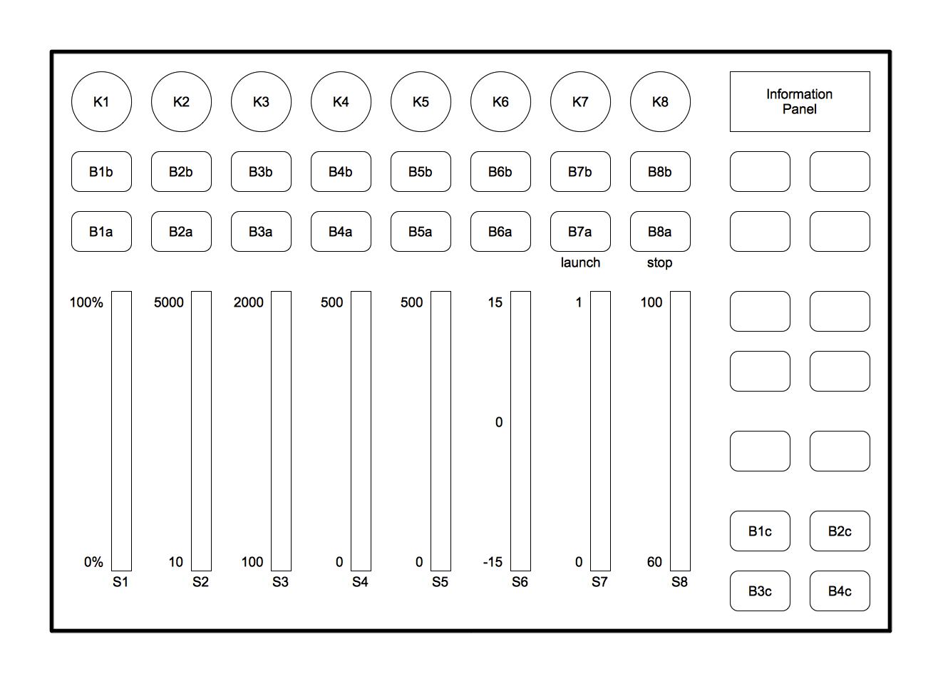
Fig. 13. Assignment of parameters in the CONTROLLER with minimum and maximum values for each slider. S1 = READING POINT (measured as a % of the whole), S2 = PULSE RATE (msec.), S3 = SEGMENT LENGTH (msec.), S4 = RATE DEVIATION (msec.), S5 = JITTER (msec.), S6 = ROTATION RATE (Hz) S7 = REVERB (wet:dry ratio), S8 = GLOBAL AMPLITUDE (dB)
Variable Parameters: READING POINT (val), PULSE RATE (val), SEGMENT LENGTH (val), RATE DEVIATION (rand), JITTER (rand), ROTATION RATE (val), REVERB (val), GLOBAL AMPLITUDE (val).
Variable Parameters are distributed as seen in Fig. 13 above.
Discussion of Slider Controlled Parameters:
S1: READING POINT
This slider establishes where in the seed sound file the segmentation process begins, by extracting 6 segments from successive location begin points. Instantaneous slider location = the position of the first of the set of 6.
If one moves this slider to the end of the file, it will generate a fade out because the last segments of the file contain silence. This can provide a more elegant way out of a MATRIX CUE (or towards a new PRESET) than fading out with the GLOBAL AMPLITUDE control of S8.
The rapid and erratic use of this slider provides a diversity of material, while concentrating on local movements creates subtle variation. When a source file contains several concatenated SAMPLES, it is possible with practice to jump between these two resources reliably. Alternatively pre-set locations can be defined.
S2: PULSE RATE
This establishes the base clock rate (period in msec.) at which the value of READING POINT is polled (and the 6-segment sets are selected). In effect, this is the “tempo” of the MATRIX process. When this value is low (i.e. the interval between beats is short, the output sounds rapid), a continuous sound results.
S3: SEGMENT LENGTH
This slider controls the duration (in msec.) of the segments extracted from the seed sound file. It cannot be negative or too small. This parameter in combination with PULSE RATE determines the density or textural quality of the resulting sound. When SEGMENT LENGTH is less than PULSE RATE, some spaces or silences are created. When SEGMENT LENGTH is greater than PULSE RATE, some materials will overlap. If SEGMENT LENGTH is more than 8 times the size of PULSE RATE, this overlap is limited by the 48 available voices.
S4: RATE DEVIATION
This slider controls how irregular the pulse is. When PULSE RATE has a value low enough so as to allow for a continuous sound, the algorithm’s effect is that of timbral and textural change. When PULSE RATE has a value high enough so as to generate perceivable discrete pulses, it provides rhythmic irregularity. The maximum RATE DEVIATION in msec. is limited to 50% of the duration between pulses at any given time.
S5: JITTER
This slider controls the temporal de-correlation of sound segments within each set of six in relation to the pulse. Again, when PULSE RATE has value low enough to allow for a continuous sound, its effect is that of timbral and textural change, and when PULSE RATE has a value high enough as to generate perceivable discrete pulses, it provides for de-correlation of the perceived attack patterns, complexifying the temporal character of the output
Both JITTER and RATE DEVIATION allow for continuous change, and the effect of their use depends on the character of the source material. Segments taken from strong attacks allow for articulate precision, creating unpredictable rhythms as JITTER and RATE DEVIATION increase. Alternatively, segments taken from the sustain or decay of a sound, particularly when combined with higher SEGMENT LENGTHS, can be used to create timbres and textures with shifting vitality as JITTER and RATE DEVIATION increase.
S6: ROTATION RATE
ROTATION RATE is the frequency in hertz of the rotation of output channels across speaker positions. This value is polled at each PULSE RATE clock tick. When the slider is at its center, the frequency is 0 Hz and there is no movement. When the slider is above the center, rotation is clockwise and when it is below, anti-clockwise. Please refer to the MATRIX spatialization section below.
S7: REVERB
This parameter helps smooth textures that are undesirably incisive. It also generates a sense of change in perceived room acoustics and the sense of space.
This parameter controls the aggregate impact of the algorithmic output. The use of this slider needs to be very carefully managed to avoid coarse effects. When a fade out is desired, it is usually more elegant to use the end button and let the samples die out through scarcity. When a general reduction of the amplitude of the cue is desired, it is more elegant and organic to reduce the density of the algorithm through combinations of PULSE RATE and SEGMENT LENGTH or by approaching the end of the file with READING LOCATION, rather than to use GLOBAL AMPLITUDE.
General Description:
THINNR begins with the variable-speed (but non-detuning) playback of an audio file. It then processes that playback by selectively removing strong spectral peaks, using two filter bands that are controlled by the performing computer musician This process leaves low amplitude spectral content, likely to be inharmonic or aperiodic (noisy) sounds, unaffected, as well as some strong spectral peaks remaining outside the filter bands. The THINNR algorithm output is consistent with the original but has a vestigial nature, and the movement of remaining spectral peaks can be reminiscent of the behavior of vocal formants over time.
Variable-speed playback is accomplished with a phase-vocoder algorithm, a common approach to variable-speed playback without pitch transposition. The phase-vocoder used here is modeled after the “Phase-vocoder time bender” from Miller Puckette's Theory and Technique of Electronic Music (World Scientific Press, 2007).
The remainder of this page is intentionally left blank.
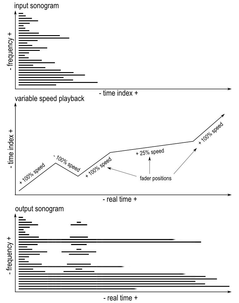
Fig. 14. Variable-speed playback with a phase-vocoder. Sonograms (frequency content plotted over time) rather than spectrograms (amplitude plotted over frequency) are used to depict the changing frequency content of a sound over time. Gradations in amplitude are not shown.
The phase-vocoder allows the effective decoupling of frequency content from the passage of time. In THINNR, a fader controls the rate at which a metaphoric playhead moves through the content of the original sound file. The performer can read through the file at 100% of the sound's normal playback speed, forward or in reverse, and at any speed between, including a speed of 0, or nearly motionless (see Fig. 14). Thus, the performer can effectively “freeze” the playhead, maintaining the spectral content of the sound at a particular time index indefinitely.
Fig. 15. Top: A possible THINNR input spectrum (amplitude plotted over frequency), with spectral peaks above a set threshold (open circles) located. Middle: an attenuation curve calculated from the locations of the most important spectral peaks. Note that this curve is calculated from points (open circles) that are inversely proportional to the peaks of the input spectrum. Bottom: Spectral output of the attenuation curve acting on the input spectrum.
As the variable-speed playback occurs, the output of the phase-vocoder is spectrally analyzed. Spectral peaks are located at each time-step of the analysis (depicted with open circles in Fig. 15). And a fixed, user-specified number of the loudest spectral peaks is used to create an attenuation curve (the curve which corresponds to some of the identified peaks in the middle of Fig. 15). Spectral peaks not ranked among the fixed number of those identified do not affect the attenuation curve (depicted as filled circles in Fig. 15). This attenuation curve is eventually applied to the output of the phase-vocoder using a bank of filters, as detailed below. However, it is best to ensure that the contour of this attenuation curve changes as smoothly as possible over time in order to prevent artifacts. This can be done by utilizing a voice allocation algorithm, which ensures maximum continuity in frequency over time for each filter, when ordering the spectral peaks used to control the filter bank
The attenuation curve (middle of Fig. 15) is applied to the input spectrum, reducing the amplitude of the loudest spectral peaks, leaving quieter peaks unaffected (marked with filled circles in Fig. 15). The lower amplitude map is the output of the filtering process. The unaffected spectral peaks are likely to be inharmonic or aperiodic components of the sound, such as key clicks, noise from the grain of a bow stroke, or breath sounds.
The previously described filtering process is not applied to the entire input spectrum. Instead, it is applied selectively to the input spectrum in two independently controlled ranges, which can be thought of as band-reject filters 1 and 2. Each has a controllable center frequency and range, and their effects are combined together (Fig. 16).
Fig. 17. Performer controlled filter bands selectively apply the attenuation of the filter bank.
The performer-controlled “formant” filter bands (middle, filters 1 + 2, Fig. 17) selectively allow two regions of the attenuation pattern created by the preliminary filter bank’s suppression (top, Fig. 17) to pass through It should be noted that because of this selection process, not all of the preliminary filter bank’s suppression will actually be heard This creates two complex band-reject filters that interact, creating resultant suppression that attenuates strong spectral peaks according to simultaneously unfolding processes (bottom, final filter, Fig. 17). These two band-reject filters can be used to perceptually isolate a region in between the two filter center frequencies that is un-attenuated, sometimes taking on “formant” like characteristics. This stage of the process has further repercussions on the spatialization strategies used: the three regions partitioned by the filter center frequencies (one low, one in the middle, and one high) are output separately (low, medium and high output, Fig. 17), resulting in parallel but distinctive spectral streams that can be independently spatialized by either ARC-TRIAD or FLOCK-SPAT.
Fig. 18 The final, filtered output (bottom) parallels the unfiltered input spectrum (top), but with some of the loudest spectral peaks selectively thinned-out by the complex, dual-band-reject filter process (middle)
THINNR produces its final output in a similar process to that depicted in Fig. 15. However, in the final output (see Fig. 18), more of the original input spectrum can potentially be present because only some of the filter bank is applied to the input, due to the performer controlled filter bands detailed in Fig. 16 and
17 First, as in Fig. 15, a select number of the loudest spectral peaks are marked for attenuation (open circles, Fig. 18, top), while many quieter spectral peaks are marked to remain (filled circles, Fig. 18, top)
Instead of rejecting all of the loudest spectral peaks, only those that fall within the performer controlled filter bands are rejected (open circles, Fig. 18, middle), leaving the quieter spectral peaks, in addition to those loud spectral peaks outside of the filter ranges (filled circles, Fig. 18, middle). This has the potential to leave many more unaffected spectral peaks in the final output (filled circles, Fig. 18, bottom). The routing of this final spectrum to the three output partitions is also depicted in Fig. 18
Performance:
THINNR has two discrete (on/off) controls, as does SMEARZ: LAUNCH, which initiates a CUE, and STOP. When the STOP button is pressed, the CONTROLLER’s sliders stop altering their respective parameters, and a fade-out of pre-determined length is initiated. The variable-speed playback continues at the same rate until the fade-out is completed.
As with PROLIF and SMEARZ, THINNR has sets of both fixed and variable parameters. Fixed parameters are set for each CUE. Variable parameters are given initialized values, but can be modified during performance using the CONTROLLER. All variables can involve continuously graduated values.
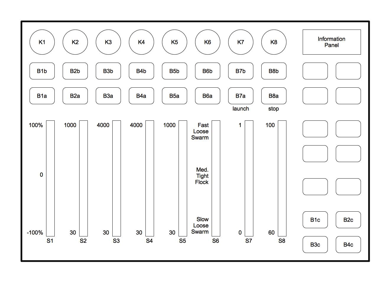
Fig. 19. Assignment of variables to the controller with minimum and maximum values for each slider. S1 = READING RATE, S2 = Q OF FILTER BAND 1 (Hz), S3 = FILTER BAND 1 CENTER FREQUENCY (Hz), S4 = FILTER BAND 2 CENTER FREQUENCY (Hz), S5 = Q OF FILTER BAND 2 (Hz), S6 = MIGRATION RATE (cf. SPATIALIZATION below), S7 = REVERB (wet:dry ratio), S8 = GLOBAL AMPLITUDE (dB).
Visual Feedback:
Visual feedback available to the computer musician during performance includes: (1) The instantaneous map of all slider positions, (2) the information panel at the top right of the CONTROLLER, which shows the current MIDI value of an active slider, (3) the output spectrum of the processed sound and the locations of the two filters bands are shown on a spectral display in the graphical user interface (GUI) of the algorithm on the computer screen. The GUI also contains a slider depicting the “playhead” or reading position in the sound file and a number box depicting the current READING RATE. These allow the performer to precisely position the filter bands, and to anticipate the approaching end of the file.
Fixed Parameters: LAUNCH POINT, SLEW TIME
LAUNCH POINT is the initial reading position or “playhead” position in the audio file.
SLEW TIME is a fixed parameter that can be initialized generally for the patch or for a new CUE. It controls how long it takes for the CENTER FREQUENCY and Q parameters of FILTER BANDS 1 and 2 to change when input from a slider is received. The default is 1000 msec.
Variable Parameters: READING RATE, Q OF FILTER BAND 1, FILTER BAND 1 CENTER FREQUENCY, FILTER BAND 2 CENTER FREQUENCY, Q OF FILTER BAND 2, MIGRATION RATE, REVERB, GLOBAL AMPLITUDE
Variable parameters are distributed on the controller as seen above in Fig. 19
Discussion of Slider Controlled Parameters:
S1: READING RATE
In THINNR, one can move the READING RATE slider in any direction at any time. 0 is at the slider’s mid-point. If the slider is set and remains unchanged, the file will be read at a constant rate from that point to the end (or, alternatively, the beginning) of the file.
- The rate at which the audio file is read can vary between the original audio file rate, through a “frozen” state (near 0 setting), to the negative of the original audio file rate.
- If set between 0 (frozen) and +100%, movement is forwards in the file.
- If set between 0 and -100%, movement is backwards.
See Fig. 14 for an illustration of the effect of the reading rate fader position.
S2: FILTER BAND 1 Q
The FILTER BAND 1 Q slider controls how wide a band is carved from the input sound's global spectrum over time. The narrowest width is approximately 30 Hz, while the widest is approximately 1000 Hz. The adjacent FILTER BAND 1 CENTER FREQUENCY slider controls its center frequency Operator input is affected by SLEW TIME.
S3: FILTER BAND 1 CENTER FREQUENCY
The FILTER BAND 1 CENTER FREQUENCY slider controls the Hertz frequency location of BAND 1. Around this center frequency, spectral peaks remaining after the preliminary suppression are removed, while low amplitude spectral content is retained. The range of center frequencies is from 30 to 4000 Hz, approximately the range of musically useful instrumental fundamental frequencies. The filter bandwidth is controlled by the adjacent FILTER BAND 1 Q slider. Operator input is affected by SLEW TIME.
S4: FILTER BAND 2 CENTER FREQUENCY
The FILTER BAND 2 CENTER FREQUENCY slider controls the Hertz frequency location of BAND 2. The adjacent FILTER BAND 2 slider controls the bandwidth The range of center frequencies is from 30 to 4000 Hz. Operator input is affected by SLEW TIME.
S5: FILTER BAND 2 Q
The FILTER BAND 2 Q slider controls how wide a band is carved from the input sound's global spectrum over time. The narrowest width is approximately 30 Hz, while the widest is approximately 1000 Hz. The adjacent FILTER BAND 2 CENTER FREQUENCY slider controls its center frequency. Operator input is affected by SLEW TIME.
S6: MIGRATION RATE
As in both PROLIF and SMEARZ, MIGRATION RATE controls the speed and character of the spatialization of THINNR’s algorithmic output, using either one of two different strategies covered in the SPATIALIZATION section. Each of the three spectral partitions of THINNR are spatialized differently, with the lowest, darkest partition moving slower in a confined space, the middle partition moving faster in a larger space, and the highest, brightest partition moving very fast in a very large space. See the SPATIALIZATION section below.
S7: REVERB
As in the other algorithms, this slider increases the ratio of reverberated (wet) to un-reverberated (dry) signal. Reverberation, in the case of THINNR, enables the whispery, thinned-out remnants of the processed sounds to bloom in a virtual acoustic space, giving them more palpability. Like PROLIF and SMEARZ, the three outputs of THINNR, one below the FILTER BAND 1 CENTER FREQUENCY, one between the FILTER BAND CENTER FREQUENCIES, and one above the FILTER BAND 2 CENTER FREQUENCY are each reverberated and spatialized differently. The lowest and darkest gets the least reverb, the middle gets a medium amount of reverb, and the highest, brightest region gets the most reverb.
This slider controls the aggregate impact of the algorithmic output. In common with the other algorithms described above, the use of this slider needs to be very carefully managed. When a fade out is desired, it is more elegant to use the STOP button. When a general reduction of the amplitude of the cue is desired it is more elegant and organic to radically thin-out the sound by increasing the Q factors, by positioning the CENTER FREQUENCIES where both filters will attenuate the largest number of spectral peaks, or by moving the READING RATE parameter to the maximum, causing the phase vocoder to finish playing the seed file.
Sound spatialization is a significant element in allowing the algorithms discussed here to achieve their optimal impact in concert. Each algorithm has a distinctive character and requires, as a result, its own choreographic signature:
PROLIF nests angularly dispersed individual points (replications of the sound source seed) in a virtual cloud of activity that then itself moves this “cloud” at various rates, and with varied continuity throughout the performance space. This might be thought of as parallel to the individual movements of birds in a flock that is itself, swooping and darting across the sky.
SMEARZ produces three-layered, blurred and extended versions of source musical gestures. The three component layers of each reconfigured sound move in differing ways so that the spectral distensions and misalignments are paralleled in the spatial representation of the smeared sonic gesture.
MATRIX depends for its character on the phenomenon of patterned iteration. Identical and closely related sounds are replicated in patterns with (usually) subtle temporal offset. The vividness with which these iterations and successions can be heard, and the way in which the totality is then made sense of, depends upon their spatial distinctiveness.
THINNR produces three layers – vestigial remnants – of musical gestures, organized by frequency range. The three component layers correspond with the frequency ranges below the low band-reject filter, between the low and high band-reject filters, and above the high bandreject filter
The four algorithms generate various audio outputs: SMEARZ gives three independent outputs per source processed, PROLIF gives up to 96 voices which are repackaged into three groups, THINNR produces three independent outputs, and MATRIX outputs 6 independent channels
SMEARZ, PROLIF and THINNR use primarily either ARC-TRIAD or FLOCK -SPAT described below.
ARC-TRIAD algorithm
General Description:
This spatialization process consists of two stages, in which the available outputs are given (1) three basic movement patterns, (2) the defining vertices of which are assigned to specific speakers and migrated through a multi-channel speaker setup (in which the number of speakers is an integer multiple of 3).
1. The purpose of this stage is to create basic movement patterns. Three output channels from an algorithm are conceptually placed at three virtual speaker locations 120 degrees from one another. This arrangement is thought of as a triad of dissemination points placed along an arc (hence, ARC-TRIAD).
A sound source output is passed from one speaker to the next clockwise or counter-clockwise, describing a virtual circle. Sounds can travel around this path as independent points or as stereo axes 180 degrees apart. This process is portrayed in Fig. 20
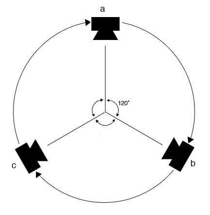
Fig. 20. Three output channels created by SMEARZ (or the three parallel output groups associated with PROLIF) are assigned to virtual speakers a, b and c. In this example, a rotation movement is then applied such that the content of a moves to b, b to c, and c to a, and so on.
It is worth noting that the speakers seen in Fig. 20 are not actual speakers in the concert space, but virtual speakers by means of which a basic source movement is generated. The speed and direction of rotation are presets loaded when launching a CUE.
2. The second stage of this spatialization strategy consists in (i) allocating an ARC-TRIAD (or its equivalent first stage movement patterns) to actual speakers and (ii) migrating this original pattern of dissemination points to other locations across the field of available speakers.
The ARC-TRIAD – which already reflects a virtual rotational movement – consists of three sound sources (a, b and c) that need to be assigned to actual speakers. In the following examples, a 12-channel setup is assumed
Speaker assignment is achieved through a bounded random process. A first speaker is randomly chosen. The second and third speakers must be either 1 or 2 positions distant from the first. A higher probability is given to speakers that are closer to the initial speaker, however, sometimes speakers are still in use and so cannot be re-assigned. They are then assigned greater inter-speaker distances.
In Fig. 21 we can see an initial triad of speakers (1, 3 and 12) to which sources a, b and c have been assigned. When assigned, the rotation generated in the first stage is represented as shown by the curved arrows. It is also worth noting that although this rotation was generated with the presumption of a 120˚ distribution, this is no longer the case and therefore the idealized circle is misshapen.
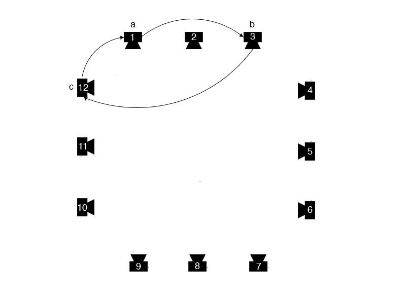
Fig. 21. The basic movement patterns from stage (1) are assigned to specific speakers.
The next step is migration. A target set of speakers is found, following the random process described above while avoiding the use of speakers from the previous set. After the allocation of sources a, b and c to the first triad of selected speakers, the next target triad is identified: a’, b’ and c’. As seen in Fig. 22, the process of migration here consists in transferring source a from speaker 1 to speaker 6, b from 3 to 7 and c from 12 to 8. The rate at which this process is iterated (i.e., a third triad is chosen and the sound sources transferred again) is controlled by a random process bounded by a minimum time (preset at 500ms) and a variable called MIGRATION RATE, which sets the maximum time duration over which an output channel is transferred from one position to the next.
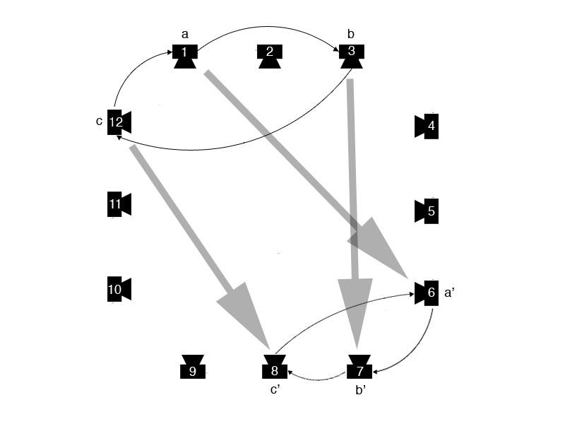
22. Migrating sources a, b and c to the target set of speakers [6, 7, 8].
The aggregate result of this two-stage process involves the migration of already spatially varied information so that existing entities (e.g., a swirling sound-cloud) migrate throughout the available space: it is a choreography of motions. An important advantage of this strategy can be found in its ability to adapt itself to widely varying performance circumstances: not only to standard concert halls, but to much larger, and more irregular shapes that might be found in public spaces such as the Library of Congress’ Great Hall, or the atrium of I. M Pei’s East Wing of the National Gallery of Art.
The process of migration can also be achieved in succession. That is, instead of moving all three sources at the same time, they move one after the other. This strategy is particularly helpful in SMEARZ, where a sense of continuous, but independently changing set of movements is desired.
Hence, the global motion allows basic movements patterns from stage 1 to migrate across the total output speaker array, as cloudlike drifting. In effect, the basic movement patterns are the content of unpredictable, global migration patterns.
General Description:
This spatialization process is an alternative to ARC-TRIAD that can also be used when a circular array of speakers is available for sound diffusion. A circular array is needed because, unlike ARC-TRIAD, FLOCK-SPAT relies on roughly simulating an artificial space around the listeners, one in which sound events occur in particular sorts of patterns. The ARC-TRIAD concept is retained, in that the three output channels of PROLIF, SMEARZ or THINNR can be placed into this space at locations that are continuously moving However, their locations are unmoored from exact speaker locations through the simulation of space, utilizing psychoacoustic cues to create the perception of depth in addition to changing direction. The migration concept is also extended; the three algorithmic outputs move as would a murmuration of starlings, utilizing concepts from flocking algorithms.
FLOCK-SPAT consists of two stages, in which the available outputs are given (1) movement patterns through a flocking algorithm, and (2) spatialized, with depth cues, through a multi-channel speaker setup.
1. Flocking algorithms are simulations that utilize distributed-agency decision-making in order to create life-like flocking behaviors. Flocking behavior can be simulated using only three forces They abstract choices and actions typically made by real animals moving in naturally occurring flocks. The basic forces are separation, cohesion and alignment. Separation and cohesion act roughly in opposition to each other, although separation tends to be felt only at short distances, and is inversely proportional to distance, while cohesion acts over greater distances, and is directly proportional to distance Agents affected by the basic forces seek to be separated by a certain distance from their neighbors in order to avoid “mid-air” collisions (see Fig. 23 top-left), but they also seek to be not too far from the center of the flock in order to “avoid predators” and to “participate in feeding” (see Fig. 23 top-right) They seek to align their trajectories at some angle in relationship to their nearest neighbors, which assists in collision avoidance (see Fig. 23 bottom-left) Roughly parallel alignments create behaviors typically associated with flocking birds or schooling fish, while roughly perpendicular alignments create behaviors associated with chaotically swarming bugs (these categories inform the way multiple behaviors are controlled in a nonlinear fashion by the MIGRATION RATE fader, found in the PROLIF, SMEARZ and THINNR algorithms – see below) In addition to the basic three forces, a force that confines the virtual flock within a defined boundary is typically implemented in order to keep the flock optimally centered (see Fig. 23 bottom-right)
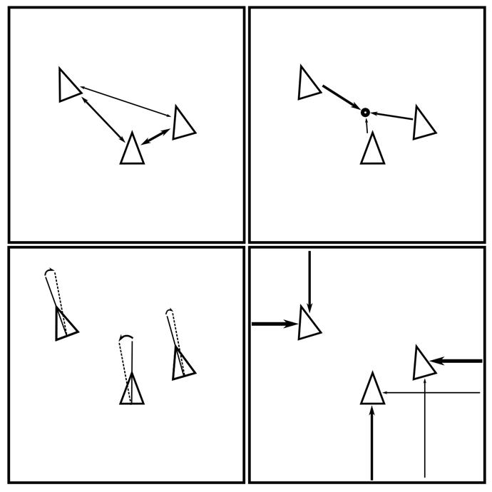
Fig. 23 Forces, depicted as arrows, governing the steering behaviors of flocking agents, depicted as triangles: separation (top-left), cohesion (top-right), alignment (bottom-left), bounding (bottom-right). Relative size of arrows illustrates relative magnitude of forces. Dotted lines indicate the average heading of the three agents, to which all agents attempt to align.
The three flocking agents in FLOCK-SPAT each carry one of the algorithmic outputs of PROLIF, SMEARZ or THINNR. One benefit of utilizing a flocking algorithm to control the spatialization of sounds is that the separation force prevents sound events from clotting particular regions of a virtual space, and instead lends toward spatially differentiated sound streams.
There are several additional strategies implemented in FLOCK-SPAT that either improve the perceptual force of the spatial movement by means of the nature of the sonic material, or contribute to ease of performance: (a) register-based speed dispositions, (b) amplitude-based individual speeds, (c) a non-linear relationship between the MIGRATION-RATE fader position and flocking behavior, and (d) a quasiperiodic “breeze” function.
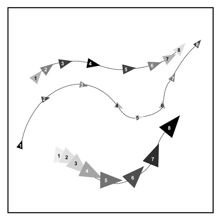
Fig. 24 Eight successive, numbered time steps (each represented by a triangle, showing agent position and orientation at that time step) in the evolution of three hypothetical agent flight paths (represented by dotted lines). Register-based speed dispositions are depicted with relative agent sizes: the larger the agent, the lower the sonic material, and the slower the speed of movement. Note how the smallest, highest agent is able to traverse a longer flight path in eight time units than the two lower voices, because it is travelling at a higher speed. Amplitude-based individual speeds are depicted with triangle shading: the darker the agent at any time step, the louder the agent is, and the more distance is traversed until the next time point/event
a. Register-based speed dispositions: the three agents generated by the algorithm are not identical in behavior. Because the algorithmic outputs are ordered in low, medium and high frequency ranges, each necessarily produces low, medium or high sounds. These frequency ranges correspond with relative agent speeds. For instance, the agent assigned to carry low frequencies has a low maximum speed, while the agent assigned to carry high frequencies has a high maximum speed (see Fig. 24).
b. Amplitude-based individual speeds: all of the flocking agents respond to the sonic material they are carrying by changing their speed in proportion to the amplitude of that sonic material. Loud sounds move faster, and quiet sounds move slower (see Fig. 24).
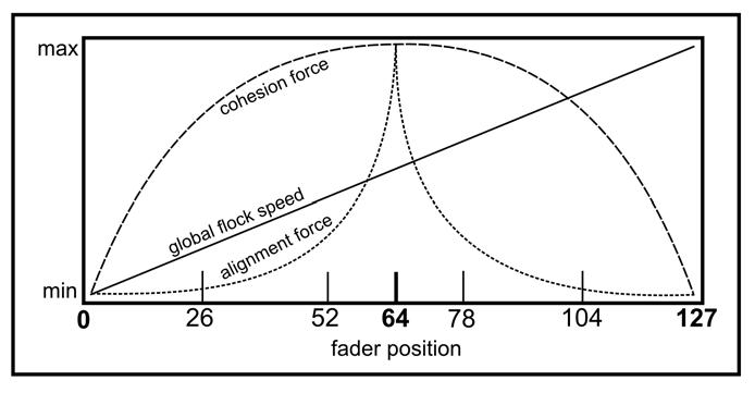
Fig. 25. Diagram depicting the relationship of the MIGRATION-RATE fader position to three FLOCK-SPAT parameters.
c. Non-linear MIGRATION-RATE fader: in PROLIF, SMEARZ and THINNR, the MIGRATION-RATE fader not only increases the speed at which agents in FLOCK-SPAT move, but it also controls several other flocking behaviors in a non-linear fashion. At a fader position of 0, the group of agents does not move. As the fader approaches the half-way point from 0 of 64, the overall speed increases to half the maximum value, while the alignment force increases exponentially to a maximum, and the cohesion force increases logarithmically to a maximum value. As the fader approaches 127 (from 64), the alignment and cohesion forces decrease in a reverse fashion from which they increased, while the overall speed reaches its maximum (see Fig. 25). This creates the impression of five loosely defined categories of flocking behavior based on fader position:
0 to 26 (slowest loose swarm): the group is sluggish, agents move randomly in relation to each other and are very dispersed around the space
26 to 52 (slower tight swarm): the group is slightly animated, agents move randomly in relation to each other but cohere into a tighter group
52 to 78 (medium tight flock): the group is moderately animated, agents align their movements with each other and cohere into a very tight group
78 to 104 (faster tight swarm): the group is very animated, agents move randomly in relation to each other but continue to cohere into a tighter group
104 to 127 (fastest loose swarm): the group is extremely animated, agents move randomly in relation to each other and are very dispersed around the space
d. Quasi-periodic “breeze” function: this provides irregular, reoccurring changes to the global behavior of the flock, in essence causing them to markedly increase the dynamism of movement change briefly. This is accomplished by occasionally increasing the maximum speed of the low and medium agent-streams in relation to that of the high agent-stream, drastically increasing overall flock speed, while increasing alignment and cohesion so that the flock sweeps in orderly formations. In the current implementation, these breezes are between 7 and 10 seconds long, and are 20 to 35 seconds apart.
2. The second stage of the FLOCK-SPAT spatialization strategy consists of rendering flocking agent positions in a virtual space around the listener. There are numerous strategies for rendering sounds in a virtual space, such as vector-based amplitude panning and ambisonics. However, because of the improbability, when touring different performance venues of ensuring perfect loudspeaker arrangements or obtaining exact spatial measurements of those arrangements, FLOCK-SPAT utilizes simple but robust amplitude-based panning order to create strong impressions of spatial movement without aiming for “holophonic” realism. In the current implementation, four or eight loudspeakers arranged roughly into a circle around the audience are optimal.
While amplitude panning in a ring of speakers sufficiently represents the directionality of sounds, depth must also be addressed. Our methods of creating depth cues involve the exaggerated use of reverberation and high frequency filtering in order to create a hyper-realistic space, rather than a merely realistic space, in which sounds occur. The exaggerated use of reverberation entails over-emphasizing the dry signal and unrealistically reducing the reverberant signal for very intimate, close sounds, while over-emphasizing the reverberant signal and greatly reducing the dry signal for distant sounds. Similarly, aggressive filtering of high frequencies aids greatly in cuing a sensation of large distances In both cases, the effect is almost surreal – the very characteristics of the virtual space change depending on the distance a sound is away from the listener.
General Description:
As MATRIX was conceived as a pattern generation engine, and depends upon multiple presentations of strongly related material over time, the spatialization for this algorithm needs to provide perceptual clarity in several ways:
• It needs to disseminate each sonic component of the output from a different position in the virtual space of the speaker field, thereby insisting upon the centrality of discrete repetition as an algorithmic feature
• The repetitions need to have, themselves, regular and easily distinguished position sequences. Thus, the fact that a structure of 6 adjacent elements from the source sound file are being repeatedly sounded takes on a deeper level of significance in that these repetitions, while potentially synchronous temporally (when not modified by JITTER) are nevertheless repositioned at each pulse of the global metronome.
• In short, the patterns of reiterated order are complemented by patterns of reiterating positions, relating temporal to spatial contiguousness.
The spatialization strategy for MATRIX consists in assigning its 6 output channels to specific loudspeakers within the available array, and determining the trajectory of these assignments over time.
As seen earlier, the six output channels contain temporally successive sound segments. These segments are assigned to spatially contiguous speakers. There need, therefore, to be as many speaker positions as there are segments in an extracted set.
The remainder of this page is intentionally left blank.
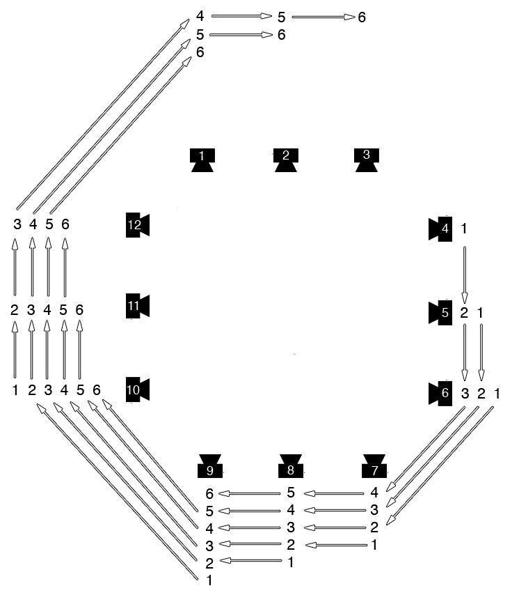
Fig. 26. Assignment of the six output channels to 12 available speakers, moving clockwise from position 4 to position 10.
For example, as seen in Fig. 26, assume there is an array of twelve loudspeakers. The numbers around the perimeter of this array depict the assignment of MATRIX output channels (each containing a sound segment) to loudspeaker locations. Arrows connect six output channels into “cascades,” showing their temporal succession. Furthermore, the multiple cascades depicted radiating outward in Fig. 26 occur one after another, rotating clockwise and ascending in starting loudspeaker location
In MATRIX, slider 6 controls ROTATION RATE. It is measured in hertz and represents the frequency of the rotation. The first position is determined at random. The center of the slider represents a frequency of 0 and therefore no movement. If the slider is moved up, the frequency of rotation increases causing a clockwise rotation of positions, while if the slider is moved down the frequency of rotation increases negatively and therefore produces a counter-clockwise rotation.
The PULSE RATE parameter also effects rotation. Each pulse of the global metronome triggers a cascade, and, as specified earlier in this document, PULSE RATE controls the speed of this metronome.
Understanding how the PULSE RATE, ROTATION RATE and JITTER parameters mutually influence the spatialization requires several figures that privilege time rather than space (Fig. 27-32) For the purpose of explication, we will assume RATE DEVIATION to be zero in these figures
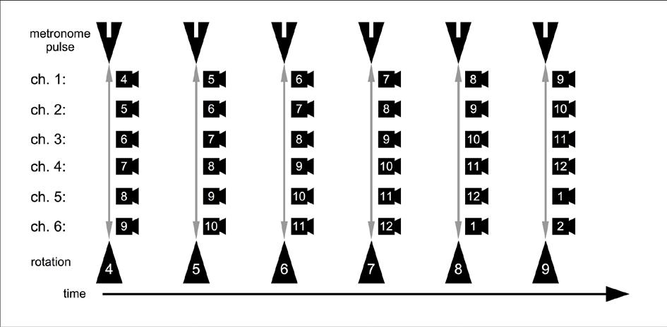
Fig. 27. MATRIX spatialization with PULSE RATE and ROTATION RATE equal to each other, with no JITTER. Each metronome pulse, depicted by heavy arrows (top), triggers a nearly simultaneous cascade of sound segments, carried by the six output channels. These six output channels are assigned to contiguous speaker groups (middle), that increase in starting position with each rotation (bottom).
Basic MATRIX spatialization, with RATE DEVIATION and JITTER set to zero, diffused with an array of twelve loudspeakers, is depicted in Fig. 27. This is the same behavior depicted in Fig. 26, but the spatial information in Fig. 27 is depicted solely with speaker numbers Each pulse of the global MATRIX metronome triggers a nearly simultaneous cascade that results in the re-positioning of six successive segments from the seed file, with each segment positioned in a successive loudspeaker, in ascending order (or in descending order for negative ROTATION RATES) With ROTATION RATE equal to the PULSE RATE, the starting speaker of each pulse is rotated by one position, in ascending order
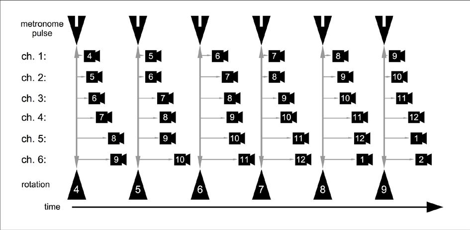
Fig. 28. MATRIX spatialization, with the same settings as Fig. 27, but with maximum JITTER.
By increasing JITTER to the maximum amount, each segment from the seed file is delayed by a random amount within the duration between metronome pulses (depicted by small, grey, horizontal arrows in Fig. 28) Segments remain sequentially ordered, as do speaker assignments The delays cause the segments to become temporally distinct, and thus the spatial trajectories become easier to hear.
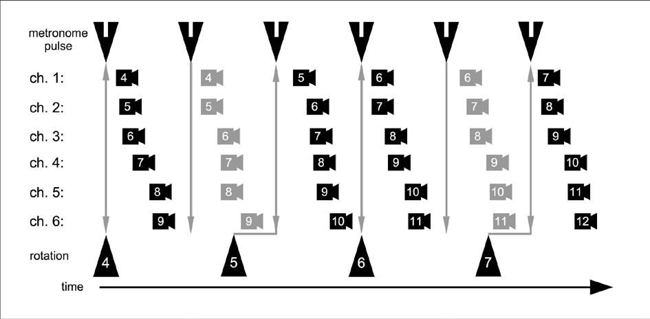
Fig. 29. MATRIX spatialization with a 2:3 rotation to pulse ratio. Grey speaker locations are the same as on previous pulses.
With all other parameters the same, slowing the ROTATION RATE to a 2:3 ratio with the PULSE RATE clarifies some of the behaviors of the MATRIX spatialization strategy. The starting speaker location for each cascade of sound segments is only updated at each metronome pulse, preserving the adjacency of all successive speaker locations within a cascade. If the rotation increments midway during a cascade, as it does during the second and fifth pulses of Fig. 29 (depicted in grey), the new rotation doesn’t go into effect (i.e., the new positions are not assigned) until the following cascade. Thus, the speaker locations of the second and fifth pulses depicted in Fig. 29 are the same as at the previous pulse.
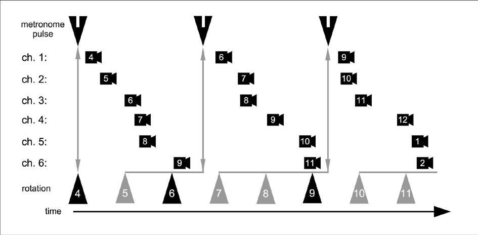
Fig. 30. MATRIX spatialization with an 8:3 ratio of rotations to pulses. Grey rotations do not go into effect because they are overridden by later rotations.
Changing the rates so that eight rotations occur for every three metronome pulses, fewer rotations go into effect (depicted in black of Fig. 30), with several rotations remaining unheard (depicted in grey). This creates perceived rotations that skip forward by varying amounts, with starting positions [4, 6, 9 ] rather than [4, 5, 6 ].
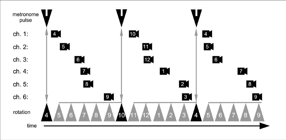
Fig. 31. MATRIX spatialization with a 6:1 rotation to pulse ratio.
By under-sampling the ROTATION RATE with the PULSE RATE, repeating successions of speaker locations can occur. For instance, with twelve loudspeakers in a ring, a ROTATION RATE six-times faster than the PULSE RATE will create repeating cascades of segments on alternating sides of a room (depicted in Fig. 31, with starting speaker positions repeating the cycle [4, 10, 4, 10 ]).
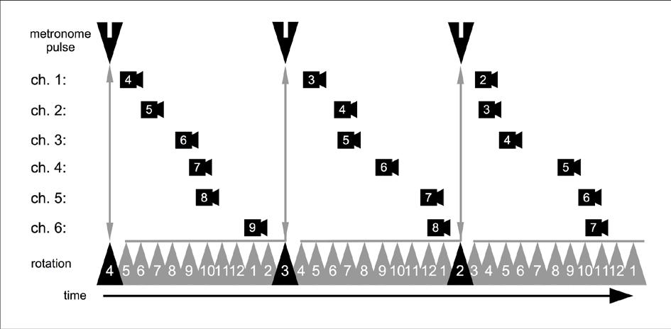
Fig. 32. MATRIX spatialization with an 11:1 rotation to pulse ratio.
Even more drastic under-sampling of the ROTATION RATE by the PULSE RATE can cause the impression that the rotation has reversed direction, (as depicted in Fig. 32) with starting speaker positions descending
As can be seen in Fig. 27 to 32, the mutual interdependence of ROTATION RATE and PULSE RATE on MATRIX spatialization creates potential for numerous types of spatial patterns. Simple, whole number ratios are less likely in performance due to the inevitable inaccuracies of manual fader repositioning, but this is in fact musically beneficial: more complex ratios typically produce the most interesting patterns, such as Fig. 30’s asymmetrically advancing rotation, due to the 8:3 rotation to pulse ratio.
Dissemination can be achieved through a multi-channel system with the minimum of 6 speakers, though 8 – 12 is preferred. If 4 speakers are unavoidable, it is possible to create a virtual representation of 8 speakers within a 4-speaker space.
The MATRIX spatialization algorithm always provides 12 channels of output and due to the discrete nature of the algorithm, these can be reassigned to smaller number of outputs as long as the continuity of the circular distribution is maintained. Since ARC-TRIAD produces 3 discrete migrating outputs the spatialization strategy is not dependent on circular setups as is usually the case plain with simple rotation algorithms where a perfect circularity and a specific number of speakers is mandatory.
For example, if 12 channels are reassigned to 6 channels, the circle of 12 sources will wrap around twice, and when reassigned to 8 channels, the circle of 12 sources will have an overlap of four. In the past, we have achieved this by allocating the overlapping 4 in a frontal disposition. The downside of using less than 12 speakers is then that there is chance that a component of the ARC-TRIAD might migrate to the same speaker, however, this has proven to be an interesting result as well.
To achieve a satisfying balance between the live performers and the electronics, the live sources are usually amplified. When the hall is resonant and/or small enough, instruments may not require amplification. If amplification is desired, the instruments should be localized so as to account for their actual positions in the hall. It is generally desirable to have an external effects processor to provide a global reverberation for both live sources and electronics as to insure blending.
November 2014
Roger Reynolds, University Professor, Department of Music, UCSD
Jaime E. Oliver, Assistant Professor of Music, NYU
Paul Hembree, Research Assistant, Department of Music, UCSD
The authors wish to thank the California Institute for Telecommunications and Information Technologies, and the Department of Music, at the University of California, San Diego for facilities, funding and collaborative assistance.
For information Contact: info@rogerreynolds.com la.rosa@nyu.edu paul.j.hembree@outlook.com