Differential equations an introduction to modern methods and applications 3rd edition brannan soluti

Differential Equations An Introduction to Modern Methods and Applications 3rd Edition

Full download link at: https://testbankpack.com/p/solution-manualfor-differential-equations-an-introduction-to-modern-methods-andapplications-3rd-edition-by-brannan-isbn-11185317799781118531778/

Chapter 7

Nonlinear Differential Equations and Stability

7.1 Autonomous Systems and Stability

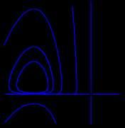
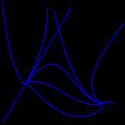
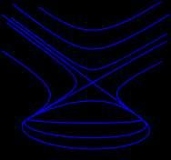
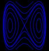
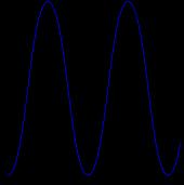
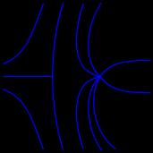
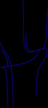
1.(a) 2y +xy = 0 implies y( 2+x) = 0 implies x = 2 or y = 0. Then, x +4xy = 0 implies x(1 + 4y) = 0 implies x = 0 or y = 1/4. Therefore, the critical points are (2, 1/4) and (0, 0).

(b)

(c) The critical point (0, 0) is a center, therefore, stable. The critical point (2, −1/4) is a saddle point, therefore, unstable.

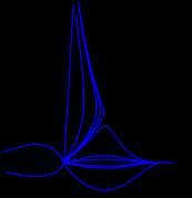
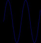
2.(a) 1 + 5y = 0 implies y = 1/5. Then, 1 6x2 = 0 implies x = ±1/ √ 6. Therefore, the critical points are (−1/ √ 6,−1/5) and (1/ √ 6,−1/5).

(c) The critical point ( 1/ √ 6, 1/5) is a saddle point, therefore, unstable. The critical point (1/ √ 6, 1/5) is a center, therefore, stable.

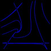
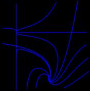
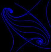
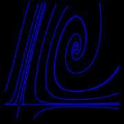
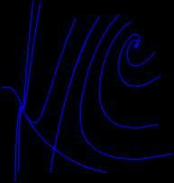
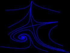
3.(a) The equation 2x x2 xy = 0 implies x = 0 or x+y = 2. The equation 3y 2y2 3xy = 0 implies y = 0 or 3x + 2y = 3. Solving these equations, we have the critical points (0, 0), (0, 3/2), (2, 0), and ( 1, 3).

(b)

(c) The critical point (0, 0) is an unstable node. The critical point (0, 3/2) is a saddle point, therefore, unstable. The critical point (2, 0) is an asymptotically stable node. The critical point ( 1,3) is an asymptotically stable node.

(d) For (2, 0), the basin of attraction is the first quadrant plus the region in the fourth quadrant bounded by the trajectories heading away from (0, 0) but looping back towards (2, 0). For (−1, 3), the basin of attraction is bounded to the right by the y−axis and to the left by those trajectories leaving (0, 0) but looping back towards ( 1, 3).

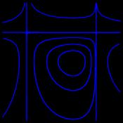
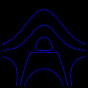
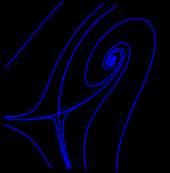
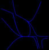
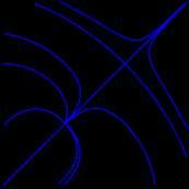
4.(a) The equation (x y)(4 x y) = 0 implies x y = 0 or x + y = 4. The equation x(2+ y) = 0 implies x = 0 or y = 2. Solving these equations, we have the critical points (0, 0), (0, 4), ( 2, 2), and (6, 2).

(c) The critical point (0, 0) is an asymptotically stable spiral point. The critical point (0, 4) is a saddle point, therefore, unstable. The critical point ( 2, 2) is a saddle point, therefore, unstable. The critical point (6, 2) is a saddle point, therefore, unstable.

(d) For (0, 0), the basin of attraction is bounded below by the line y = 2, to the right by a trajectory passing near the point (5, 0), to the left by a trajectory heading towards (and then away from) the unstable critical point (0, 4), and above by a trajectory heading towards (and then away from) the unstable critical point (0, 4).

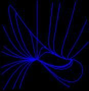
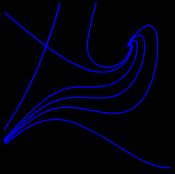
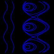
5.(a) The equation x(6 − x − y) = 0 implies x = 0 or x + y = 6. If x = 0, the equation x + 7y 2xy = 0 implies y = 0. If x + y = 6, then the equation x + 7y 2xy = 0 can be reduced to y2 2y 3 = 0. Therefore, y = 1 or y = 3. Now if y = 1, then x = 7. If y = 3, then x = 3. Therefore, the critical points are (0, 0), (7, 1), and (3, 3).

(b)

(c) The critical point (0, 0) is an unstable node. The critical point (3, 3) is a saddle point, therefore, unstable. The critical point (7, 1) is an asymptotically stable spiral point.

(d) For (7, 1), the basin of attraction is bounded to the left by the y axis and above by the trajectories heading into the unstable critical point (3, 3).

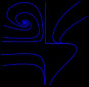
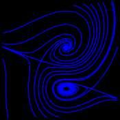
6.(a) The equation (2 x)(y x) = 0 implies x = 2 or x = y. The equation y(2 x x2) = 0 implies y = 0 or x = 2 or x = 1. The solutions of those two equations are the critical points (0, 0), (2, 0), ( 2, 2), and (1, 1).

(c) The critical point (0, 0) is a saddle point, therefore, unstable. The critical point (2, 0) is also a saddle point, therefore, unstable. The critical point ( 2, 2) is an asymptotically stable spiral point. The critical point (1, 1) is also an asymptotically stable spiral point.

(d) For ( 2, 2), the basin of attraction is the region bounded above by the x-axis and to the right by the line x = 2. For (1, 1), the basin of attraction is the region bounded below by the x-axis and to the right by the line x = 2.

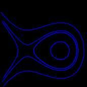
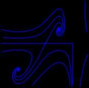
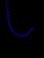
7.(a) The equation (2 y)(x y) = 0 implies y = 2 or x = y. The equation (1+x)(x+y) = 0 implies x = 1 or x = y The solutions of those two equations are the critical points (0, 0), ( 1,2), ( 2,2), and ( 1, 1).

(b)

(c) The critical point (0, 0) is an unstable spiral point. The critical point ( 1, 2) is a saddle point, therefore, unstable. The critical point ( 2, 2) is an asymptotically stable spiral point. The critical point ( 1, 1) is a saddle point, therefore, unstable.

(d) For ( 2, 2), the basin of attraction is a circular region lying mainly in the second quadrant, close to the x and y-axes, bounded by trajectories leaving the unstable spiral point (0, 0) and approaching the saddle ( 1, 2).

8.(a) The equation x(2 x y) = 0 implies x = 0 or x+y = 2. The equation (1 y)(2+x) = 0 implies y = 1 or x = 2. The solutions of those two equations are the critical points (0, 1), (1, 1), and ( 2, 4).

(c) The critical point (0, 1) is a saddle point, therefore, unstable. The critical point (1, 1) is an asymptotically stable node. The critical point ( 2,4) is an unstable spiral point.

(d) For (1, 1), the basin of attraction is the right half plane

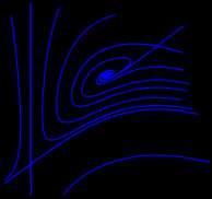
9.(a) The equation (3+x)(2y x)= 0 implies x = 3 or x = 2y. The equation (2 x)(y x) = 0 implies x = 2 or x = y. The solutions of these two equations are the critical points (0, 0), (2, 1), and ( 3, 3).

(b)

(c) The critical point (0, 0) is an asymptotically stable spiral point. The critical point (2, 1) is a saddle point, therefore, unstable. The critical point ( 3, 3) is also a saddle point, therefore, unstable.

(d) The basin of attraction of (0, 0) is bounded by the trajectories approaching the saddle point (2, 1).

10.(a) The equation (1+y)(1−x) = 0 implies x = 1 or y = −1. If x = 1, then x−12y−x2 = 0 implies that y = 0. If y = 1, then x 12y x2 = 0 implies that x2 x 12 = 0, thus x = 3 or x = 4. Therefore, the critical points are (1, 0), ( 3, 1), and (4, 1).

(c) The critical point (1, 0) is a saddle point, therefore, unstable. The critical point ( 3, 1) is an unstable node. The critical point (4, 1) is an asymptotically stable node.

(d) The basin of attraction for (4, 1) is bounded above by the trajectory heading towards and then away from the unstable critical point (1, 0). The basin is bounded on the left by a trajectory travelling away from the unstable critical point ( 3, 1).

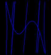
11.(a) The equation y = 0 implies y = 0. Then ify = 0, the equation 3y x(x 1)(x 2) = 0 reduces to x = 0,1,2. Therefore, the critical points are (0, 0), (1, 0), and (2, 0).

(b)

(c) The critical point (0, 0) is a saddle point, therefore, unstable. The critical point (1, 0) is an asymptotically stable node. The critical point (2, 0) is a saddle point, therefore, unstable.

(d) The basin of attraction for (1, 0) is bounded on the left by trajectories heading towards and then away from the unstable critical point (0, 0). The basin is bounded on the right by trajectories traveling towards and then away from the unstable critical point (2, 0).

12.(a) The critical points are ( 2,1), ( 2,1/2), (2, 1), and (1/3, 2/3).

7.1. AUTONOMOUS SYSTEMS AND STABILITY 505

(c) The critical point (−2, 1) is an unstable node. The critical point (−2, 1/2) is a saddle point, therefore, unstable. The critical point (2, 1) is a saddle point, therefore, unstable. The critical point (1/3, 2/3) is an asymptotically stable spiral point.

(d) The basin of attraction for (1/3, 2/3) is bounded on the left by the line x = 2 and bounded above by the line y = 1.

13.(a) The equation dx/dt= 0 implies x = 0 or x +3y = 8. The equation dy/dt = 0 implies y = 0, x = 3, or x = 2. Solving these two equations simultaneously, we see that the critical points are (0, 0), (8, 0), (3, 5/3), and (−2,10/3).

(b)

(c) The critical point (0, 0) is an unstable node. The critical point (3, 5/3) is a saddle point, therefore, unstable. The critical point (8, 0) is an asymptotically stable node. The critical point ( 2,10/3) is a saddle point, therefore, unstable.

(d) The basin of attraction for (8, 0) is the fourth quadrant plus the part of the first quadrant to the right of the two solutions approaching the saddle point (3, 5/3).

14.(a) The equation dx/dt = 0 implies y = 1 or x 2y = 1. The equation dy/dt = 0 implies y = 0 or 2x + y = 3. Solving these two equations simultaneously, we see that the critical points are (2, 1), ( 1,0), and (1, 1).

(c) The critical point (2, 1) is an asymptotically stable spiral point. The critical point ( 1, 0) is a saddle point, therefore, unstable. The critical point (1, 1) is an unstable spiral point.

(d) The basin of attraction for (2, 1) is bounded above by the x-axis, and from the left by the solution approaching the saddle point ( 1, 0).

15.(a) The equation dx/dt = 0 implies y = 1, x = 1 or x = 2. The equation dy/dt = 0 implies x = 0 or y = 2. Solving these two equations simultaneously, we see that the critical points are (0, 1), (1, 2), and ( 2, 2).

(b)

(c) The critical point (0, 1) is a center, therefore, stable. The critical point (1, 2) is a saddle point, therefore, unstable. The critical point ( 2,2) is a saddle point, therefore, unstable.

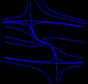
16.(a) The equation dx/dt = 0 implies y = ±5. The equation dy/dt = 0 implies x = 1 or x = y. Solving these two equations simultaneously, we see that the critical points are (1, 5), ( 5,5), (1, 5), and (5, 5).

(c) The critical point (1, 5) is a saddle point, therefore, unstable. The critical point ( 5, 5) is an unstable spiral point. The critical point (1, −5) is a saddle point, therefore, unstable. The critical point (5, 5) is an asymptotically stable spiral point.

(d) The basin of attraction for (5, 5) is bounded below and to the right by trajectories heading towards the unstable critical point (1, −5). The basin is bounded above by trajectories heading towards the unstable critical point (1, 5).

17.(a) The equation dx/dt = 0 implies y = 0. The equation dy/dt = 0 implies x = 0 or x = ±

6 Solving these two equations simultaneously, we see that the critical points are (0, 0), (

6,0), and ( √ 6,0). (b)

(c) The critical point (0, 0) is a saddle point, therefore, unstable. The critical point ( √ 6, 0) is a center, therefore, stable. The critical point ( √ 6,0) is a center, therefore, stable.

18.(a) The equation dy/dt = 0 implies y = 0 or x = 1/2. Using these values in the equation for dx/dt= 0, we see that the critical points are (0, 0), (1, 0), and (1/2,1/4).

(c) The critical point (0, 0) is a saddle point, therefore, unstable. The critical point (1, 0) is a saddle point, therefore, unstable. The critical point (1/2,1/4) is a center, therefore, stable.

19.(a) The trajectories are solutions of the differential equation

Rewriting this equation as ω2 sinx dx + ydy = 0, we see that this differential equation is exact with

Integrating the first equation, we find that H(x, y) = ω2 cosx + f(y). Differentiating this equation with respect to y, we find that Hy = f0(y) = y which implies that f(y) = y2/2+C. Therefore, the solutions of the differential equation are level curves of

Adding an arbitrary constant does not affect the trajectories. Therefore, the trajectories can be written as

where C is an arbitrary constant.

(b) Multiplying by mL2 and reverting to the original physical variables, we obtain

Since ω2 = g/L, this equation can be written as where

7.1. AUTONOMOUS SYSTEMS AND STABILITY 509 CHAPTER 7. NONLINEAR DIFFERENTIAL EQUATIONS AND STABILITY

(c) The absolute velocity of the point mass is given by v = Ldθ/dt The kinetic energy of the mass is T = mv2/2. Choosing the rest position as the datum, that is, the level of zero potential energy, the gravitational potential energy of the point mass is V = mgL(1 cosθ). It follows that the total energy, T + V , is constant along the trajectories.

20.(a) Since the system is undamped, and y(0) = 0, the amplitude is 0.25. The period is estimated at τ ≈ 3.16.

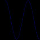
(b) In each case, the amplitudes are given by R = 0.5,1.0,1.5,2.0, respectively. The periods T are estimated at 3.20,3.35,3.63,4.17, respectively

(c) Since the system is conservative, the amplitude is equal to the initial amplitude. The period of motion is an increasing function of the initial position A.

It appears that as A → 0, the period approaches π, the period of the corresponding linear pendulum.

7.1. AUTONOMOUS SYSTEMS AND STABILITY 510 CHAPTER 7. NONLINEAR DIFFERENTIAL EQUATIONS AND STABILITY

(d) The pendulum is released from rest at an inclination of 4 π radians from vertical. The pendulum will swing past the lower equilibrium position (θ = 2π) and come to rest, momentarily, at a maximum rotational displacement of θmax = 4π 4. The transition between the two dynamics occurs at A = π.

21.(a) For initial velocity v = 3, the pendulum will swing back and forth about its equilibrium position. For initial velocity v = 6, the pendulum will not swing back and forth, but instead will continue to rotate about the origin indefinitely

(b) By plotting the graphs of the solutions for different values of v, we conclude that the transition takes place at vc ≈ 4.90.

22.(a) We see that

Integrating this equation with respect to θ, we have

EQUATIONS AND STABILITY

Separating variables and taking the square root of both sides of the equation, we have

The negative square root is chosen because the bob is being released from a positive angle α. Therefore, dθ/dt will be negative.

(b) Integrating the last equation above from α to 0, we have

First, t(α) = 0, since the bob starts at θ = α Further, if the period of the pendulum is T, then the bob will first go by the equilibrium position θ = 0 at time T/4. Therefore, we conclude that

(c) By using the identities cos

we can rewrite the equation in part (b) as

Next, making the change of variables sin(θ/2) = ksinφ with k = sin(α/2), our equation becomes

(d) Set k = sin(

/2) = sin(A/2)and g/L =

23. We compute: and

dΦ dφ = dt dt dΨ dψ = dt dt

(t s) = F (φ(t s), ψ(t s)) = F (Φ,Ψ) = F (x, y) (t s) = G(φ(t s), ψ(t s)) = F (Φ,Ψ) = G(x, y).

Therefore, Φ(t),Ψ(t) is a solution for α + s < t < β + s.

24. Let C0 be the trajectory generated by the solution x = φ0(t),y = ψ0(t)with φ0(t0)= x0, ψ0(t0)= y0 and let C1 be the trajectory generated by the solution x = φ1(t), y = ψ1(t) with φ1(t1)= x0, ψ1(t1)= y0. From problem 23, we know that Φ1(t) = φ1(t− (t0 − t1)), Ψ1(t) = ψ1(t (t0 t1))is a solution. Further, Φ1(t0)= φ1(t1) = x0 and Ψ1(t0)= y0 Then, by uniqueness, φ0(t) = Φ1(t) and ψ0(t) = Φ1(t). Therefore, the trajectories must be the same.

25. If we assume that a trajectory can reach a critical point (x0, y0) in a finite length of time, then we would have two trajectories passing through the same point. This contradicts the result in problem 24.

26. Since the trajectory is closed, there is at least one point (x0, y0) such that φ(t0)= x0, ψ(t0)= y0 and a number T > 0 such that φ(t0 + T) = x0, ψ(t0+ T) = y0. From problem 23, we know that Φ(t) = ψ(t+ T), Ψ(t) = ψ(t+ T) will also be a solution. But, then by uniqueness Φ(t) = φ(t) and Ψ(t) = ψ(t) for all t. Therefore, φ(t + T) = φ(t) and ψ(t+ T) = ψ(t)for all t. Therefore, the solution is periodic with period T

7.2 Almost Linear Systems

1.(a) The equation dx/dt = 0 implies y = 2x. The equation dy/dt = 0 implies y = x2 . Therefore, for these equations to both be satisfied, we need 2x = x2 which means x = 0 or x = 2. Thus the two critical points are (0, 0) and (2, 4).

(b) Here, we have F (x, y) = −2x + y and G(x, y) = x2 − y. Therefore, the Jacobian matrix for this system is J(x,y) = Fx Fy Gx Gy = 2 1 2x 1

Near the critical point (0, 0), the Jacobian matrix is Fx(0,0) Fy(0,0) = 2 1 J(0,0) = Gx(0, 0) Gy(0, 0) 0 1

and the corresponding linear system near (0, 0) is d x 2 1 x .

y = 0 1 y

Near the critical point (2, 4), the Jacobian matrix is

and the corresponding linear system near (2, 4) is

where

(c) The eigenvalues of the linear system near (0, 0) are λ = 1, 2. From this, we can conclude that (0, 0) is an asymptotically stable node for the nonlinear system. The eigenvalues of the linear system near (2, 4) are ( 3 ± √ 17)/2. Since one of these eigenvalues is positive and one is negative, the critical point (2, 4) is an unstable saddle point for the nonlinear system.

(d)

(e) The basin of attraction for the asymptotically stable critical point (0, 0) is bounded on the right by trajectories heading towards the critical point (2, 4).

2.(a) To find the critical points, we need to solve the equations y = x and x 3y+xy 3 = 0. Plugging x in for y in the second equation, we see that we have x = 3 and x = 1. Therefore, the two critical points are (3, 3) and ( 1, 1).

(b) Here, we have F (x, y) = x y and G(x, y) = x 3y + xy 3. Therefore, the Jacobian matrix for this system is

Near the critical point (3, 3), the Jacobian matrix is

=

and the corresponding linear system near (3, 3) is

7.2. ALMOST LINEAR SYSTEMS

CHAPTER 7. NONLINEAR DIFFERENTIAL EQUATIONS AND STABILITY

where u = x 3 and v = y 3. Near the critical point ( 1, 1), the Jacobian matrix is

and the corresponding linear system near ( 1, 1) is

where u = x + 1 and v = y + 1.

(c) The eigenvalues of the linear system near (3, 3) are λ = (1 ± √ 15i)/2. From this, we can conclude that (3, 3) is an unstable spiral point for the nonlinear system. The eigenvalues of the linear system near ( 1, 1) are λ = 1, 4. Since one of these eigenvalues is positive and one is negative, the critical point ( 1, 1) is an unstable saddle point for the nonlinear system.

3.(a) To find the critical points, we need to solve the equations x = y2 and x = 2y In order for these two equations to be satisfied simultaneously, we need y2 = 2y. Therefore, y = 0 or y = 2. Therefore, the two critical points are (0, 0) and ( 4, 2).

(b) Here, we have F (x, y) = x + y2 and G(x, y) = x + 2y. Therefore, the Jacobian matrix for this system is

y) =

x Fy

x Gy

1 2y = 1 2 .

Near the critical point (0, 0), the Jacobian matrix is

0) =

x(0,0) Fy(0,0) = 1 0

x(0, 0) Gy(0, 0) 1 2

and the corresponding linear system near (0, 0) is d x 1 0 x

y = 1 2 y .

7.2. ALMOST LINEAR SYSTEMS 515

CHAPTER 7. NONLINEAR DIFFERENTIAL EQUATIONS AND STABILITY

Near the critical point ( 4,2), the Jacobian matrix is

and the corresponding linear system near ( 4,2) is

where u = x + 4 and v = y 2.

(c) The eigenvalues of the linear system near (0, 0) are λ = 1,2. From this, we can conclude that (0, 0) is an unstable node for the nonlinear system. The eigenvalues of the linear system near ( 4,2) are λ = (3 ± √ 17)/2. Since one of these eigenvalues is positive and one is negative, the critical point ( 4,2) is an unstable saddle point for the nonlinear system.

4.(a) To find the critical points, we need to solve the equations x = y2 and x 2y + x2 = 0. Plugging x = y2 into the second equation, we have y4 + y2 2y = 0. The real solutions of this equation are y = 0,1. Therefore, the two critical points are (0, 0) and (1, 1).

(b) Here, we have F (x, y) = x y2 and G(x, y) = x 2y + x2 Therefore, the Jacobian matrix for this system is

y) = Fx Fy Gx Gy = 1 2y 1 + 2x 2

Near the critical point (0, 0), the Jacobian matrix is

x(0,0) Fy(0,0) = 1 0

0) = Gx(0, 0) Gy(0, 0) 1 2

and the corresponding linear system near (0, 0) is

x 1 0 x

y = . 1 2 y

7.2. ALMOST LINEAR SYSTEMS

CHAPTER 7. NONLINEAR DIFFERENTIAL EQUATIONS AND STABILITY

Near the critical point ( 4,2), the Jacobian matrix is

Near the critical point (1, 1), the Jacobian matrix is

and the corresponding linear system near (1, 1) is

where

(c) The eigenvalues of the linear system near (0, 0) are λ = 1, 2. From this, we can conclude that (0, 0) is an unstable saddle point for the nonlinear system. The eigenvalues of the linear system near (1, 1) are λ = ( 1 ±

15i)/2. From this, we can conclude that (1, 1) is an asymptotically stable spiral point for the nonlinear system.

(e) The basin of attraction for the asymptotically stable point (1, 1) is bounded above by a trajectory heading over the spiral region, towards (0, 0) and is bounded below by a trajectory heading towards (0, 0).

5.(a) To find the critical points, we need to solve the equations (4 + x)(y x) = 0 and (10 x)(y + x) = 0. Solving this system of equations, we see that the critical points are given by (0, 0), (10,10), and ( 4, 4).

(b) Here, we have F (x, y) = (4 + x)(y x) and G(x, y) = (10 x)(y + x). Therefore, the Jacobian matrix for this system is

Near the critical point (0, 0), the Jacobian matrix is

and the corresponding linear system near (0, 0) is

7.2. ALMOST LINEAR SYSTEMS 517

CHAPTER 7. NONLINEAR DIFFERENTIAL EQUATIONS AND STABILITY

Near the critical point ( 4,2), the Jacobian matrix is

y = 10 10 y

7.2. ALMOST LINEAR SYSTEMS 517

CHAPTER 7. NONLINEAR DIFFERENTIAL EQUATIONS AND STABILITY

Near the critical point ( 4,4), the Jacobian matrix is

and the corresponding linear system near ( 4,4) is

where u = x + 4 and v = y 4. Near the critical point (10,10), the Jacobian matrix is J(10,10) = Fx(10, 10) Fy(10, 10) Gx(10, 10) Gy(10, 10) 14 14 = 20 0

and the corresponding linear system near (10,10) is d u 14 14

where u = x − 10 and v = y − 10.

(c) The eigenvalues of the linear system near (0, 0) are λ = 3 ±

89. From this, we can conclude that (0, 0) is an unstable saddle point for the nonlinear system. The eigenvalues of the linear system near ( 4, 4) are λ = 8,14. From this, we can conclude that ( 4, 4) is an unstable node for the nonlinear system. The eigenvalues of the linear system near (10,10) √ are λ = 7 ± i 231. From this, we can conclude that (10,10) is an asymptotically stable spiral point the nonlinear system.

(d)

(e) The basin of attraction for the asymptotically stable point (10, 10) is bounded below by trajectories heading in towards the origin and bounded on the left by trajectories heading away from ( 4, 4).

6.(a) To find the critical points, we need to solve the equations x x2 xy = 0 and 3y xy 2y2 = 0. Solving this system of equations, we see that the critical points are given by (0, 0), (0, 3/2), (1, 0), and (−1, 2).

7.2. ALMOST LINEAR SYSTEMS 518

CHAPTER 7. NONLINEAR DIFFERENTIAL EQUATIONS AND STABILITY

Near the critical point ( 4,4), the Jacobian matrix is

(b) Here, we have F (x, y) = x x2 xy and G(x, y) = 3y xy 2y2 Therefore, the Jacobian matrix for this system is

Near the critical point (0, 0), the Jacobian matrix is

and the corresponding linear system near (0,

is

Near the critical point (0, 3/2), the Jacobian matrix is

and the corresponding linear system near (0, 3/2) is

where u = x and v = y 3/2. Near the critical point (1, 0), the Jacobian matrix is

and the corresponding linear system near (1, 0) is

where u = x 1 and v = y. Near the critical point ( 1,2), the Jacobian matrix is

and the corresponding linear system near ( 1,2) is

7.2. ALMOST LINEAR SYSTEMS 519

CHAPTER 7. NONLINEAR DIFFERENTIAL EQUATIONS AND STABILITY

Near the critical point ( 4,4), the Jacobian matrix is

(c) The eigenvalues of the linear system near (0, 0) are λ = 1,3. From this, we can conclude that (0, 0) is an unstable node for the nonlinear system. The eigenvalues of the linear system

EQUATIONS AND STABILITY

near (0, 3/2) are λ = 1/2, 3. From this, we can conclude that (0, 3/2) is an asymptotically stable node for the nonlinear system. The eigenvalues of the linear system near (1, 0) are λ = 1,2. From this, we can conclude that (1, 0) is a saddle point for the nonlinear system. The eigenvalues of the linear system near ( 1,2) are λ = ( 3 ± √ 17)/2. From this, we can conclude that ( 1,2) is a saddle point for the nonlinear system.

(d)

(e) The basin of attraction for the asymptotically stable point (0, 3/2) consists of the first quadrant combined with trajectories heading into the second quadrant from (0, 0) and towards (0, 3/2).

7.(a) To find the critical points, we need to solve the equations 1 y = 0 and x2 y2 = 0. Solving this system of equations, we see that the critical points are given by ( 1, 1) and (1, 1).

(b) Here, we have F (x, y) = 1 y and G(x, y) = x2 y2 Therefore, the Jacobian matrix for this system is

=

Near the critical point ( 1,1), the Jacobian matrix is

Near the critical point (1, 1), the Jacobian matrix is

(c) The eigenvalues of the linear system near (−1,1) are λ = −1 ± √ 3. From this, we can conclude that ( 1, 1) is a saddle point for the nonlinear system. The eigenvalues of the linear system near (1, 1) are λ = 1±i. From this, we can conclude that (1, 1) is an asymptotically stable spiral point for the nonlinear system.

(e) The basin of attraction for the asymptotically stable point (1, 1) is bounded on the left by trajectories just to the left of the y axis and below by trajectories heading away from the saddle point ( 1,1) and back towards (1, 1).

8.(a) To find the critical points, we need to solve the equations x x2 2xy = 0 and y(x + 1) = 0. The second equation implies x = 1 or y = 0. Plugging these values into the first equation, we see that the three critical points are (0, 0), (1, 0), and ( 1, 1).

(b) Here, we have F (x, y) = x −x2 −2xy and G(x, y) = −y(x + 1). Therefore, the Jacobian matrix for this system is

Near the critical point (0, 0), the Jacobian matrix is

and the corresponding linear system near (0, 0) is

Near the critical point (1, 0), the Jacobian matrix is

and the corresponding linear system near (1, 0) is

the Jacobian matrix is

7.2. ALMOST LINEAR SYSTEMS 521 CHAPTER 7. NONLINEAR DIFFERENTIAL EQUATIONS AND STABILITY

and the corresponding linear system near ( 1,1) is d u 1 2 u

=

where u = x + 1 and v = y 1.

(c) The eigenvalues of the linear system near (0, 0) are λ = 1, 1. From this, we can conclude that (0, 0) is an unstable saddle point for the nonlinear system. The eigenvalues of the linear system near (1, 0) are λ = 1, 2. From this, we can conclude that (1, 0) is an asymptotically stable node for the nonlinear system. The eigenvalues of the linear system near ( 1,1) are λ = (1 ± √ 7i)/2. From this, we can conclude that ( 1,1) is an unstable spiral point.

(e) The basin of attraction for the asymptotically stable point (1, 0) is the right half plane.

9.(a) To find the critical points, we need to solve the equations (x y)(6 x y) = 0 and x(4 + y) = 0. Solving these equations, we find that the critical points are (0, 0), ( 4, 4), (0, 6), and (10,−4).

(b) Here, we have F (x, y) = (x y)(6 x y) and G(x, y) = x(4 + y). Therefore, the Jacobian matrix for this system is

=

Near the critical point (0, 0), the Jacobian matrix is

Near the critical point (0, 6), the Jacobian matrix is

=

Near the critical point (−4,−4), the Jacobian matrix is

4) = .

7.2. ALMOST LINEAR SYSTEMS 523 CHAPTER 7. NONLINEAR DIFFERENTIAL EQUATIONS AND STABILITY

7.2. ALMOST LINEAR SYSTEMS 524 CHAPTER 7. NONLINEAR DIFFERENTIAL EQUATIONS AND STABILITY

Near the critical point (10, 4), the Jacobian matrix is 14 14 J(10,−4) =

(c) The eigenvalues of the linear system near (0, 0) are λ = 3 ±

33. From this, we can conclude that (0, 0) is an unstable saddle point for the nonlinear system. The eigenvalues

of the linear system near (0, 6) are λ = 3 ± i 51. From this, we can conclude that

(0, 1) is an asymptotically stable spiral for the nonlinear system. The eigenvalues of the linear system near ( 4, 4) are λ = 4, 14. From this, we can conclude that ( 4, 4) is an asymptotically stable node. The eigenvalues of the linear system near (10, 4) are λ = 10,14. From this, we can conclude that (10, 4) is an unstable node.

(e) Tha basin of attraction for (0, 4) is bounded below by the two trajectories approaching (0, 0). The basin of attraction for ( 4, 4) is bounded above by the same two trajectories.

10.(a) To find the critical points, we need to solve the equations x+x2+y2 = 0 and y−xy = 0. Solving these equations, we find that the critical points are (0, 0) and ( 1, 0).

(b) Here, we have F (x, y) = x + x2 + y2 and G(x, y) = y xy Therefore, the Jacobian matrix for this system is

y) = Fx Fy Gx Gy

1 + 2x 2y = . y 1 x

Near the critical point (0, 0), the Jacobian matrix is 1 0 J(0,0) = 0 1 .

Near the critical point (−1,0), the Jacobian matrix is

7.2. ALMOST LINEAR SYSTEMS 525 CHAPTER 7. NONLINEAR DIFFERENTIAL EQUATIONS AND STABILITY

(c) The eigenvalues of the linear system near (0, 0) are λ = 1. From this, we can conclude that (0, 0) is an unstable node or spiral point for the nonlinear system. The eigenvalues of

the linear system near ( 1,0) are λ = 1,3. From this, we can conclude that ( 1,0) is a saddle point for the nonlinear system.

(d)

11.(a) To find the critical points, we need to solve the equations 2x + y + xy3 = 0 and x 2y xy = 0. Substituting y = x/(x+ 2) into the first equation results in

One root of this equation is x = 0. The only other real root is

Therefore, the critical points are (0, 0) and (approximately) (−1.19345,−1.4797).

(b) Here, we have F (x, y) = 2x+y+xy3 and G(x, y) = x 2y xy. Therefore, the Jacobian matrix for this system is

Near the critical point (0, 0), the Jacobian matrix is

Near the critical point ( 1.19345, 1.4797), the Jacobian matrix is

−

(c) The eigenvalues of the linear system near (0, 0) are λ = ± √ 5. From this, we can conclude that (0, 0) is an unstable saddle point for the nonlinear system. The eigenvalues of the linear system near ( 1.19345, 1.4797) are λ = 1.0232 ± 4.1125i. From this, we can conclude that ( 1 19345, 1 4797) is an asymptotically stable spiral point for the nonlinear system.

(e) The basin of attraction for the stable spiral point is bounded by the two trajectories approaching (0, 0).

12.(a) To find the critical points, we need to solve the equations (2 + x) siny = 0 and 1 − x − cosy = 0. If x = −2, then we must have cosy = 3, which is impossible. Therefore, sin y = 0, which implies that y = nπ, n = 0,±1,±2,... Based on the second equation, x = 1 cosnπ. It follows that the critical points are located at (0, 2kπ) and (2, (2k + 1)π) where k = 0,±1,±2,...

(b) Here, we have F (x, y) = (2+x)sin y and G(x, y) = 1−x−cosy. Therefore, the Jacobian matrix for this system is

J(x,y) = Fx Fy Gx Gy

siny (2 + x)cosy = . 1 siny

Near the critical points (0, 2kπ), the Jacobian matrix is 0 2 J(0,2kπ) = 1

Near the critical point (2, (2k + 1)π), the Jacobian matrix is

(2k + 1)π) = 0 4 . 1 0

(c) The eigenvalues of the linear system near (0, 2kπ) are λ = ± √ 2i. Based on this information, we cannot make a conclusion about the nature of the critical points near (0, 2kπ) for the nonlinear system. The eigenvalues of the linear system near (2, (2k + 1)π) are λ = ±2. From this, we can conclude that the critical points (2, (2k + 1)π) are saddles.

Upon looking at the phase portrait, we see that the critical points (0, 2kπ) are centers.

13.(a) To find the critical points, we need to solve the equations x y2 = 0 and y x2 = 0. Substituting y = x2 into the first equation, results in x x4 = 0 which has real roots x = 0,1. Therefore, the critical points are (0, 0) and (1, 1).

(b) Here, we have F (x, y) = x y2 and G(x, y) = y x2 . Therefore, the Jacobian matrix for this system is

Near the critical point (0, 0), the Jacobian matrix is

Near the critical point (1, 1), the Jacobian matrix is

(c) There is a repeated eigenvalue λ = 1 for the linear system near (0, 0). Based on this information, we cannot make a conclusion about the nature of the critical point near (0, 0) for the nonlinear system, only that it is unstable and it is either a node or a spiral. The eigenvalues of the linear system near (1, 1) are λ = 3, 1. From this, we can conclude that the critical point (1, 1) is a saddle.

(d)

Upon looking at the phase portrait, we see that the critical point (0, 0) is an unstable node.

14.(a) To find the critical points, we need to solve the equations 3 xy = 0 and x 3y3 = 0. After multiplying the second equation by y, it follows that y = ±1. Therefore, the critical points of the system are (3, 1) and ( 3, 1).

(b) Here, we have F (x, y) = 3 xy and G(x, y) = x 3y3 . Therefore, the Jacobian matrix for this system is

Near the critical point (3, 1), the Jacobian matrix is

Near the critical point ( 3, 1), the Jacobian matrix is

13. There is an asymptotically stable node here. The eigenvalues of the linear system near ( 3, 1) are 4±2

(c) The eigenvalues of the linear system near (3, 1) are λ = 5 ±

7. From this, we can conclude that the critical point ( 3, 1) is a saddle. (d)

(e) The basin of attraction for (3, 1) is bounded from the left by the two trajectories approaching ( 3, 1).

15.(a) To find the critical points, we need to solve the equations

It is clear that (0, 0) is a critical point. Solving the first equation for y, we find that

Substitution of these relations into the second equation results in two equations of the form f1(x)= 0 and f2(x)= 0. Plotting these functions, we note that only f1(x)= 0 has real roots given by x ≈ ±0.33076. It follows that the additional critical points are (approximately) ( 0.33076,1.0924) and (0.33076, 1.0924).

(b) Here, we have F (x, y) = 2x y x(x2 +y2) and G(x, y) = x y+y(x2 +y2). Therefore, the Jacobian matrix for this system is

Near the critical point (0, 0), the Jacobian matrix is

Near the critical points ( 0.33076,1.0924) and (0.33076, 1.0924), the Jacobian matrix is

1.0924) =

−1.0924)

(c) The eigenvalues of the linear system near (0, 0) are λ = ( 3 ± i

3)/2. Therefore, (0, 0) is an asymptotically stable spiral point for the nonlinear system. The eigenvalues of the linear system near ( 0 33076,1.0924) and (0.33076, 1 0924) are 3 5092,2.6771, respectively From this, we can conclude that these two critical points are saddles.

(d)

(e) The basin ofattraction for (0, 0) is bounded above and below by the solutions approaching the two saddles, respectively.

16.(a) To find the critical points, we need to solve the equations

Multiplying the first equation by y, the second equation by x and subtracting the second from the first, we conclude that x2 + y2 = 0. Therefore, the only critical point is (0, 0).

(b) Here, we have F (x, y) = y+x(1 x2 y2) and G(x, y) = x+y(1 x2 y2). Therefore, the Jacobian matrix for this system is

J(x,y) = Fx Fy Gx Gy

1 3x2 y2 1 2xy = 1 2xy 1 x2 3y2

Near the critical point (0, 0), the Jacobian matrix is 1 1 J(0,0) = . 1 1

(c) The eigenvalues of the linear system near (0, 0) are λ = 1 ± i. Therefore, (0, 0) is an unstable spiral point for the nonlinear system.

(d)

17.(a) The critical points occur when either y = 2 or y = 0.5x and either x = 2 or y = 0 5x Solving these equations simultaneously, we have the critical points (0, 0), (2, 2), (2, 1), and (4, 2).

(b) Here, we have F (x, y) = (2 + y)(y 0.5x) and G(x, y) = (2 x)(y + 0.5x). Therefore, the Jacobian matrix for this system is

J(x,y) = Fx Fy Gx Gy = 1 0.5y 2 + 2y 0.5x . y + 1 x 2 x

Near the critical point (0, 0), the Jacobian matrix is Fx(0,0) Fy(0,0) = 1 2 J(0,0) = Gx(0, 0) Gy(0, 0) 1 2

and the corresponding linear system near (0, 0) is d x 1 2 x . dt y = 1 2 y

Near the critical point (2, 2), the Jacobian matrix is Fx(2, 2) Fy(2, 2) = 0 3 J(2,−2) = Gx(2, 2) Gy(2, 2) 1 0

and the corresponding linear system near (2, 2) is

where u = x 2 and v = y + 2. Near the critical point (2, 1), the Jacobian matrix is

and the corresponding linear system near (2, 1) is

where u = x 2 and v = y 1. Near the critical point (4, 2), the Jacobian matrix is

and the corresponding linear system near (4, 2) is

(c) The eigenvalues of the linear system near (0, 0) are λ = (1 ± √ 17)/2. From this, we can conclude that (0, 0) is an unstable saddle point for the nonlinear system. The eigenvalues of the linear system near (2, 2) are λ = ± √ 3i. From this, we can only say that (2, 2) is a center or spiral point for the nonlinear system, and we do cannot determine the stability. The eigenvalues of the linear system near (2, 1) are λ = ( 3 ± √ 87i)/4. From this, we can conclude that (2, 1) is an asymptotically stable spiral point. The eigenvalues of the linear system near (4, 2) are λ = 1± √ 5. From this, we can conclude that (4, 2) is an unstable saddle point.

(d)

531 CHAPTER 7. NONLINEAR DIFFERENTIAL EQUATIONS AND STABILITY ALMOST LINEAR SYSTEMS 531

From the phase portrait, we can see that (2, 2) is a stable center for the nonlinear system.

(e) The basin of attraction for the asymptotically stable point (2, 1) is bounded to the left and below by trajectories heading towards the unstable saddle point (0, 0). The basin of attraction is bounded to the right by trajectories heading around the left side of the center (2, 2).

18.(a) The critical points occur when either y = ±2 and either x = 1.5 or x = y. Therefore, we see that the critical points are given by ( 1 5,2), (2, 2), ( 1 5, 2), and ( 2, 2).

(b) Here, we have F (x, y) = 4 y2 and G(x, y) = (1.5 + x)(y x). Therefore, the Jacobian matrix for this system is

Near the critical point (−1.5,2), the Jacobian matrix is

and the corresponding linear system near ( 1 5,2) is

Near the critical point (2, 2), the Jacobian matrix is

and the corresponding linear system near (2, 2) is

where

= x 2 and v = y 2. Near the critical point ( 1.5, 2), the Jacobian matrix is

and the corresponding linear system near ( 1.5, 2) is

where

= x + 1.5 and v = y + 2. Near the critical point ( 2, 2), the Jacobian matrix is

and the corresponding linear system near ( 2, 2) is d u 0 4 u

= 1/2 1/2 v

where u = x + 2 and v = y + 2.

(c) The eigenvalues of the linear system near ( 1 5,2) are λ = ± √ 14i. From this, we can only conclude that ( 1.5,2) is a center or a spiral point, and we cannot determine its stability. The eigenvalues of the linear system near (2, 2) are λ = (7 ± √ 273)/4. From this, we can conclude that (2, 2) is an unstable saddle point for the nonlinear system. The eigenvalues of the linear system near ( 1.5, 2) are λ = ± √ 2i. From this, we can only conclude that ( 1 5, 2) is a either a center or a spiral point, and we cannot d etermine its stability The eigenvalues of the linear system near ( 2, 2) are λ = ( 1 ± √ 33)/4. From this, we can conclude that ( 2, 2) is an unstable saddle point.

From the phase portrait above, we can see that ( 1.5,2) and ( 1.5, 2) are stable centers for the nonlinear system.

19.(a) The critical points occur when either y = 1 or y = 2x and either x = 2 or x = 2y Therefore, we see that the critical points are (0, 0), (2, 1), (−2,1), and (−2,−4).

(b) Here, we have F (x, y) = (1 y)(2x y) and G(x, y) = (2 + x)(x 2y). Therefore, the Jacobian matrix for this system is

Near the critical point (0, 0), the Jacobian matrix is

and the corresponding linear system near (0, 0) is

Near the critical point (2, 1), the Jacobian matrix is

and the corresponding linear system near (2, 1) is

where u = x − 2 and v = y − 1. Near the critical point (−2,1), the Jacobian matrix is

and the corresponding linear system near ( 2,1) is

where u = x 2 and v = y 1. Near the critical point ( 2, 4), the Jacobian matrix is

and the corresponding linear system near (

(c) The eigenvalues of the linear system near (0, 0) are λ = 1 ± √

7. From this, we can conclude that (0, 0) is an unstable saddle point for the nonlinear system. The eigenvalues of the linear system near (2, 1) are λ = 2, 6. From this, we can conclude that (2, 1) is an asymptotically stable node for the nonlinear system. The eigenvalues of the linear system near ( 2,1) are λ = ±2 √ 5i. From this, we can only conclude that ( 2,1) is a either a center or a spiral point, and we cannot determine its stability. The eigenvalues of the linear system near ( 2, 4) are λ = 5 ± √ 5i. From this, we can conclude that ( 2, 4) is an unstable spiral point.

(d)

From the phase portrait above, we can see that ( 2, 1) is a stable center for the nonlinear system.

(e) The basin of attraction for the asymptotically stable node (2, 1) is bounded on the left by trajectories approaching the stable center ( 2, 1) and also by those trajectories heading to the left away from the unstable spiral point ( 2, 4).

20.(a) Looking at the equation dy/dt = 0, we see that we need x = 0, y = 0 or y = 3. Plugging each of these values into the equation dx/dt = 0, we conclude that the critical points are (0, 0), (2, 3), and ( 2, 3).

(b) Here, we have F (x, y) = 2x2y 3x2 4y and G(x, y) = 2xy2 + 6xy. Therefore, the Jacobian matrix for this system is

Near the critical point (0, 0), the Jacobian matrix is

and the corresponding linear system near (0, 0) is

Near the critical point (2, 3), the Jacobian matrix is

and the corresponding linear system near (2, 3) is

where u = x − 2 and v = y − 3. Near the critical point (−2,3), the Jacobian matrix is

and the corresponding linear system near ( 2,3) is

where u = x + 2 and v = y 3.