Solution manual for digital signal processing using matlab a problem solving companion 4th edition b by sandra.yanchik975

Solution Manual for Digital Signal Processing Using MATLAB A Problem Solving Companion 4th Edition by Ingle Proakis ISBN 1305635124 9781305635128

Full link download:

Solution Manual: https://testbankpack.com/p/solution-manual-for-digital-signal-processing-using-matlab-a-problem-solvingcompanion-4th-edition-by-ingle-proakis-isbn-1305635124-9781305635128/

Chapter 2 Discrete-Time Signals and Systems

P2.1 Generate the following sequences using the basic MATLAB signal functions and the basic MATLAB signal operations discussed in this chapter Plot signal samples using the stem function

1. x1.n/ D 3 .n C 2/ C 2 n/ .n 3/ C 5 .n 7/, 5 n 15

% P0201a: x1(n) = 3*delta(n + 2) + 2*delta(n) - delta(n - 3) + % 5*delta(n - 7), -5 <= n <= 15. clc; close all;

x1 = 3*impseq(-2,-5,15) + 2*impseq(0,-5,15)- impseq(3,-5,15) + 5*impseq(7,-5,15);Hf_1 = figure; set(Hf 1,’NumberTitle’ , ’off’ , ’Name’ , ’P0201a’); n1 = [-5:15]; Hs = stem(n1,x1,’filled’);set(Hs,’markersize’,2);axis([min(n1)1,max(n1)+1,min(x1)-1,max(x1)+1]); xlabel(’n’ , ’FontSize’,LFS); ylabel(’x 1(n)’ , ’FontSize’,LFS); title(’Sequence x_1(n)’ , ’FontSize’,TFS); set(gca,’XTickMode’ , ’manual’ , ’XTick’,n1,’FontSize’,8); print -deps2 ../EPSFILES/P0201a;

The plots of x1.n/ is shown in Figure 2.1

6 5 4 3 2 1 0 ï1 ï2 ï5ï4ï3ï2ï1 0 1 2 3 4 5 6 7 8 9 101112131415 n

Sequence x1(n) Figure 2 1: Problem P2 1 1 sequence plot

%P0201b: x2(n) = sum {k = -5}^{5} e^{-|k|}*delta(n - 2k), -10 <= n <= 10 clc; close all;

n2 = [-10:10]; x2 = zeros(1,length(n2)); for k = -5:5

x2 = x2 + exp(-abs(k))*impseq(2*k,-10,10); end

Hf_1 = figure; set(Hf 1,’NumberTitle’ , ’off’ , ’Name’ , ’P0201b’); Hs = stem(n2,x2,’filled’);set(Hs,’markersize’,2);axis([min(n2)1,max(n2)+1,min(x2)-1,max(x2)+1]); xlabel(’n’ , ’FontSize’,LFS); ylabel(’x 2(n)’ , ’FontSize’,LFS); title(’Sequence x_2(n)’ , ’FontSize’,TFS); set(gca,’XTickMode’ , ’manual’ , ’XTick’,n2); print -deps2 ../EPSFILES/P0201b;

The plots of x2.n/ is shown in Figure 2.2.

2 SOLUTIONS MANUAL FOR DSP USING MATLAB (4TH EDITION) SOLUTIONS MANUAL FOR DSP USING MATLAB (4TH EDITION) 2 © 2017 Cengage Learning® May not be scanned, copied or duplicated, or posted to a publicly accessible website, in whole or in part © 2017 Cengage Learning® May not be scanned, copied or duplicated, or posted to a publicly accessible website, in whole or in part 2. x2.n/ D 5 X kD5 k j e .n 2k/, 10n 10.

2 1 5 1 0.5 0 −0.5 1 SEQUENCE X2(N) 10 9 8 7 6 5 4 3 2 1 0 1 2 3 4 5 6 7 8 9 10 N

Figure 2 2: Problem P2 1 2 sequence plot

%P0201c: x3(n) = 10u(n) - 5u(n - 5) + 10u(n - 10) + 5u(n - 15) clc; close all;

x3 = 10*stepseq(0,0,20) - 5*stepseq(5,0,20) - 10*stepseq(10,0,20)... + 5*stepseq(15,0,20); n3 = [0:20];

Hf_1 = figure; set(Hf 1,’NumberTitle

); Hs = stem(n3,x3,’filled’);set(Hs,’markersize’,2);axis([min(n3)1,max(n3)+1,min(x3)-1,max(x3)+2]); ytick = [-6:2:12];

xlabel(’n’ , ’FontSize’,LFS); ylabel(’x 3(n)’ , ’FontSize’,LFS); title(’Sequence x 3(n)’ , ’FontSize’,TFS);

set(gca,’XTickMode’ , ’manual’ , ’XTick’,n3); set(gca,’YTickMode’ , ’manual’ , ’YTick’,ytick); print -deps2 ./EPSFILES/P0201c;

The plots of x3.n/ is shown in Figure 2.3

3 SOLUTIONS MANUAL FOR DSP USING MATLAB (4TH EDITION) SOLUTIONS MANUAL FOR DSP USING MATLAB (4TH EDITION) 3 © 2017 Cengage Learning® May not be scanned, copied or duplicated, or posted to a publicly accessible website, in whole or in part © 2017 Cengage Learning® May not be scanned, copied or duplicated, or posted to a publicly accessible website, in whole or in part 3. x3.n/ D 10u n/ 5u.n 5/ 10u n 10/ C 5u n 15/.

’ , ’off’ , ’Name’ , ’P0201c’

SEQUENCE X3(N) 12 10 8 6 4 2 0 −2 −4 −6 0 1 2 3 4 5 6 7 8 9 1011121314151617181920 N

Figure 2 3: Problem P2 1 3 sequence plot

%P0201d: x4(n) = e ^ {0.1n} [u(n + 20) - u(n - 10)]. clc; close all;

n4 = [-25:15];

x4 = exp(0.1*n4) *(stepseq(-20,-25,15) - stepseq(10,-25,15));

Hf_1 = figure; set(Hf 1,’NumberTitle’ , ’off’ , ’Name’ , ’P0201d’); Hs = stem(n4,x4,’filled’);set(Hs,’markersize’,2);axis([min(n4)-2,max(n4)+2,min(x4)1,max(x4)+1]); xlabel(’n’ , ’FontSize’,LFS); ylabel(’x 4(n)’ , ’FontSize’,LFS);

title(’Sequence x 4(n)’ , ’FontSize’,TFS);ntick = [n4(1):5:n4(end)]; set(gca,’XTickMode’ , ’manual’ , ’XTick’,ntick);

print -deps2 ./CHAP2 EPSFILES/P0201d; print -deps2 ./. /Latex/P0201d; The plots of x

is shown in Figure

4 SOLUTIONS MANUAL FOR DSP USING MATLAB (4TH EDITION) SOLUTIONS MANUAL FOR DSP USING MATLAB (4TH EDITION) 4 © 2017 Cengage Learning® May not be scanned, copied or duplicated, or posted to a publicly accessible website, in whole or in part © 2017 Cengage Learning® May not be scanned, copied or duplicated, or posted to a publicly accessible website, in whole or in part 0:1n 4. x4.n/ D e u.n C 20/ u.n 10/

4.n/

2.4. SEQUENCE X4(N) 3 2.5 2 1 5 1 0.5 0 0 5 1 25 20 15 10 5 0 5 10 15 N

Figure 2 4: Problem P2 1 4 sequence plot

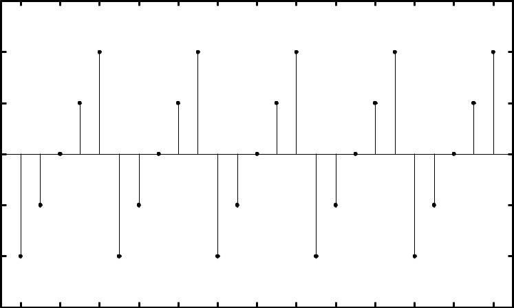
5. x5.n/ D 5 cos.0:49 n/ C cos.0:51 n/ ; 200 n 200 Comment on the waveform shape

%P0201e: x5(n) = 5[cos(0.49*pi*n) + cos(0.51*pi*n)], -200 <= n <= 200 clc; close all;

n5 = [-200:200]; x5 = 5*(cos(0.49*pi*n5) + cos(0.51*pi*n5));

Hf_1 = figure; set(Hf 1,’NumberTitle’ , ’off’ , ’Name’ , ’P0201e’); Hs = stem(n5,x5,’filled’);set(Hs,’markersize’,2);axis([min(n5)10,max(n5)+10,min(x5)-2,max(x5)+2]); xlabel(’n’ , ’FontSize’,LFS); ylabel(’x 5(n)’ , ’FOntSize’,LFS); title(’Sequence x_5(n)’ , ’FontSize’,TFS);

ntick = [n5(1): 40:n5(end)]; ytick = [-12 -10:5:10 12]; set(gca,’XTickMode’ , ’manual’ , ’XTick’,ntick); set(gca,’YTickMode’ , ’manual’ , ’YTick’,ytick); print -deps2 ./CHAP2 EPSFILES/P0201e; print -deps2 ./. /Latex/P0201e;

The plots of x5.n/ is shown in Figure 2.5

5 SOLUTIONS MANUAL FOR DSP USING MATLAB (4TH EDITION) SOLUTIONS MANUAL FOR DSP USING MATLAB (4TH EDITION) 5 © 2017 Cengage Learning® May not be scanned, copied or duplicated, or posted to a publicly accessible website, in whole or in part © 2017 Cengage Learning® May not be scanned, copied or duplicated, or posted to a publicly accessible website, in whole or in part

SEQUENCE X5(N) 12 10 5 0 5 −10 12 200 160 120 80 40 0 40 80 120 160 200 N

Figure 2 5: Problem P2 1 5 sequence plot

6. x6.n/ D 2 sin 0:01 n/ cos.0:5 n/; 200 n 200

%P0201f: x6(n) = 2 sin(0.01*pi*n) cos(0.5*pi*n), -200 <= n <= 200. clc; close all;

n6 = [-200:200]; x6 = 2*sin(0.01*pi*n6).*cos(0.5*pi*n6);

Hf_1 = figure; set(Hf 1,’NumberTitle’ , ’off’ , ’Name’ , ’P0201f’); Hs = stem(n6,x6,’filled’);set(Hs,’markersize’,2);axis([min(n6)10,max(n6)+10,min(x6)-1,max(x6)+1]); xlabel(’n’ , ’FontSize’,LFS); ylabel(’x 6(n)’ , ’FontSize’,LFS); title(’Sequence x_6(n)’ , ’FontSize’,TFS); ntick = [n6(1): 40:n6(end)];

set(gca,’XTickMode’ , ’manual’ , ’XTick’,ntick); print -deps2 ../CHAP2 EPSFILES/P0201f; print -deps2 ../../Latex/P0201f; The plots of x6.n/ is shown in Figure 2.6

6 SOLUTIONS MANUAL FOR DSP USING MATLAB (4TH EDITION) SOLUTIONS MANUAL FOR DSP USING MATLAB (4TH EDITION) 6 © 2017 Cengage Learning® May not be scanned, copied or duplicated, or posted to a publicly accessible website, in whole or in part © 2017 Cengage Learning® May not be scanned, copied or duplicated, or posted to a publicly accessible website, in whole or in part X 6 ( N )

3 2 1 0 1 2 3 200 160 120 80 40 0 40 80 120 160 200 N

SEQUENCE X6(N)

Figure 2.6: Problem P2.1.6 sequence plot

0:05n 7. x7.n/ D e sin.0:1 n C =3/; 0 n 100

%P0201g: x7(n) = e ^ {-0 05*n}*sin(0 1*pi*n+ pi/3), 0 <= n <=100 clc; close all;

n7 = [0:100]; x7 = exp(-0 05*n7) *sin(0 1*pi*n7 + pi/3);

Hf_1 = figure; set(Hf 1,’NumberTitle’ , ’off’ , ’Name’ , ’P0201g’); Hs = stem(n7,x7,’filled’);set(Hs,’markersize’,2);axis([min(n7)5,max(n7)+5,min(x7)-1,max(x7)+1]); xlabel(’n’ , ’FontSize’,LFS); ylabel(’x 7(n)’ , ’FontSize’,LFS); title(’Sequence x_7(n)’ , ’FontSize’,TFS);

ntick = [n7(1): 10:n7(end)]; set(gca,’XTickMode’ , ’manual’ , ’XTick’,ntick); print -deps2 ../CHAP2 EPSFILES/P0201g;

The plots of x7.n/ is shown in Figure 2.7

7 SOLUTIONS MANUAL FOR DSP USING MATLAB (4TH EDITION) SOLUTIONS MANUAL FOR DSP USING MATLAB (4TH EDITION) 7 © 2017 Cengage Learning® May not be scanned, copied or duplicated, or posted to a publicly accessible website, in whole or in part ©

Cengage Learning® May not be scanned, copied or duplicated, or posted to a publicly accessible website, in whole or in part

2017

EQUENCE X7(N) 1 5 1 0.5 0 0 5 −1 1 5 0 10 20 30 40 50 60 70 80 90 100 N

Figure 2 7: Problem P2 1 7 sequence plot

0:01n 8. x8.n/ D e sin.0:1 n/; 0 n 100.

% P0201h: x8(n) = e ^ {0.01*n}*sin(0 1*pi*n),0 <= n <=100. clc; close all;

n8 = [0:100]; x8 = exp(0 01*n8) *sin(0 1*pi*n8);

Hf_1 = figure; set(Hf 1,’NumberTitle’ , ’off’ , ’Name’ , ’P0201h’); Hs = stem(n8,x8,’filled’);set(Hs,’markersize’,2);axis([min(n8)5,max(n8)+5,min(x8)-1,max(x8)+1]); xlabel(’n’ , ’FontSize’,LFS); ylabel(’x 8(n)’ , ’FontSize’,LFS); title(’Sequence x_8(n)’ , ’FontSize’,TFS);

ntick = [n8(1): 10:n8(end)]; set(gca,’XTickMode’ , ’manual’ , ’XTick’,ntick); print -deps2 ../CHAP2 EPSFILES/P0201h

The plots of x8.n/ is shown in Figure 2.8.

8 SOLUTIONS MANUAL FOR DSP USING MATLAB (4TH EDITION) SOLUTIONS MANUAL FOR DSP USING MATLAB (4TH EDITION) 8 © 2017 Cengage Learning® May not be scanned, copied or duplicated, or posted to a publicly accessible website, in whole or in part ©

Cengage Learning® May not be scanned, copied or duplicated, or posted to a publicly accessible website, in whole or in part

2017

SEQUENCE X8(N) 3 2 1 0 −1 2 −3 0 10 20 30 40 50 60 70 80 90 100 N Figure 2 8: Problem P2 1 8 sequence plot

P2.2 Generate the following random sequences and obtain their histogram using the hist function with 100 bins Use the bar function to plot each histogram.

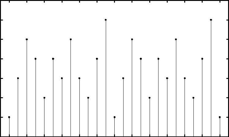
1. x1.n/ is a random sequence whose samples are independent and uniformlydistributed over 0; 2 interval Generate 100,000 samples

%P0202a: x1(n) = uniform[0,2] clc; close all;

n1 = [0:100000-1]; x1 = 2*rand(1,100000);

Hf_1 = figure; set(Hf 1,’NumberTitle’ , ’off’ , ’Name’ , ’P0202a’); [h1,x1out] = hist(x1,100); bar(x1out, h1); axis([-0.1 2.1 0 1200]);

xlabel(’interval’, ’FontSize’,LFS); ylabel(’number of elements’ , ’FontSize’,LFS); title(’Histogram of sequence x_1(n) in 100 bins’ , ’FontSize’,TFS); print -deps2 ./CHAP2 EPSFILES/P0202a;

The plots of x1.n/ is shown in Figure 2.9.

9 SOLUTIONS MANUAL FOR DSP USING MATLAB (4TH EDITION) SOLUTIONS MANUAL FOR DSP USING MATLAB (4TH EDITION) 9 © 2017 Cengage Learning® May not be scanned, copied or duplicated, or posted to a publicly accessible website, in whole or in part © 2017 Cengage Learning® May not be scanned, copied or duplicated, or posted to a publicly accessible website, in whole or in part

1200 1000 800 600 400 200 0

(n) in

0 0 2 0 4 0 6 0 8 1 1 2 1 4 1 6 1 8 2 interval

Histogram

sequence x1

100 bins

Figure 2 9: Problem P2 2 1 sequence plot

2. x2.n/ is a Gaussian random sequence whose samples are independent with mean 10 and variance 10 Generate 10,000 samples.

%P0202b: x2(n) = gaussian{10,10} clc; close all;

n2 = [1:10000]; x2 = 10 + sqrt(10)*randn(1,10000);

Hf_1 = figure; set(Hf 1,’NumberTitle’ , ’off’ , ’Name’ , ’P0202b’); [h2,x2out] = hist(x2,100); bar(x2out,h2); xlabel(’interval’ , ’FontSize’,LFS); ylabel(’number of elements’ , ’FontSize’,LFS);

title(’Histogram of sequence x_2(n) in 100 bins’ , ’FontSize’,TFS);print -deps2 ../CHAP2 EPSFILES/P0202b;

The plots of x2.n/ is shown in Figure 2.10.

10 SOLUTIONS MANUAL FOR DSP USING MATLAB (4TH EDITION) SOLUTIONS MANUAL FOR DSP USING MATLAB (4TH EDITION) 10 © 2017 Cengage Learning® May not be scanned, copied or duplicated, or posted to a publicly accessible website, in whole or in part © 2017 Cengage Learning® May not be scanned, copied or duplicated, or posted to a publicly accessible website, in whole or in part

400 350 300 250 200 150 100 50

0 −5 0 5 10 15 20 25 interval

Histogram of sequence x2(n) in 100 bins

Figure 2.10: Problem P2.2 2 sequence plot

3. x3.n/ D x1.n/ C x1.n 1/ where x1.n/ is the random sequence given in part 1 above. Comment on the shape of this histogram and explain the shape.

%P0202c: x3(n) = x1(n) + x1(n - 1) where x1(n) = uniform[0,2] clc; close all;

n1 = [0:100000-1]; x1 = 2*rand(1,100000);

Hf_1 = figure; set(Hf 1,’NumberTitle’ , ’off’ , ’Name’ , ’P0202c’); [x11,n11] = sigshift(x1,n1,1); [x3,n3] = sigadd(x1,n1,x11,n11);[h3,x3out] = hist(x3,100); bar(x3out,h3); axis([-0.5

4.5 0 2500]);

xlabel(’interval’ , ’FontSize’,LFS);

ylabel(’number of elements’ , ’FontSize’,LFS);

title(’Histogram of sequence x_3(n) in 100 bins’ , ’FontSize’,TFS);print -deps2 ../CHAP2 EPSFILES/P0202c;

The plots of x3.n/ is shown in Figure 2.11.

of sequence x3(n) in 100 bins

11 SOLUTIONS MANUAL FOR DSP USING MATLAB (4TH EDITION) SOLUTIONS MANUAL FOR DSP USING MATLAB (4TH EDITION) 11 © 2017 Cengage Learning® May not be scanned, copied or duplicated, or posted to a publicly accessible website, in whole or in part © 2017 Cengage Learning® May not be scanned, copied or duplicated, or posted to a publicly accessible website, in whole or in part

2500 2000 1500 1000 500

0 −0.5 0 0.5 1 1.5 2 2.5 3 3.5 4 4.5 interval

Histogram Figure 2.11: Problem P2.2 3 sequence plot

4. x4.n/ D P4 kD1 yk.n/ where each random sequence yk n/ is independent of others with samples uniformly dis-tributed over 0:5; 0:5 . Comment on the shape of this histogram.

%P0202d: x4(n) = sum {k=1} ^ {4} y k(n), where each independent of others % with samples uniformlydistributed over [-0.5,0.5]; clc; close all;

y1 = rand(1,100000) - 0 5; y2 = rand(1,100000) - 0 5; y3 = rand(1,100000) - 0 5; y4 = rand(1,100000) - 0 5; x4 = y1 + y2 + y3 + y4;

Hf_1 = figure; set(Hf 1,’NumberTitle’ , ’off’ , ’Name’ , ’P0202d’); [h4,x4out] = hist(x4,100); bar(x4out,h4); xlabel(’interval’ , ’FontSize’,LFS); ylabel(’number of elements’ , ’FontSize’,LFS);

title(’Histogram of sequence x_4(n) in 100 bins’ , ’FontSize’,TFS);print -deps2 ../CHAP2 EPSFILES/P0202d;

The plots of x4.n/ is shown in Figure 2.12.

12 SOLUTIONS MANUAL FOR DSP USING MATLAB (4TH EDITION) SOLUTIONS MANUAL FOR DSP USING MATLAB (4TH EDITION) 12 © 2017 Cengage Learning® May not be scanned, copied or duplicated, or posted to a publicly accessible website, in whole or in part © 2017 Cengage Learning® May not be scanned, copied or duplicated, or posted to a publicly accessible website, in whole or in part

3000 2500 2000 1500 1000 500 Histogram of sequence x4(n) in 100 bins 0 2 1.5 1 0.5 0 0.5 1 interval

1 5 2

Figure 2 12: Problem P2 2.4 sequence plot

P2.3 Generate the following periodic sequences and plot their samples (using the stem function) over the indicated number of periods

1. xQ1.n/ D f: : : ; 2;1; 0; 1; 2; : : :gperiodic Plot 5 periods "

%P0203a: x1(n) = {...,-2,-1,0,1,2,-2,-1,0,1,2...}periodic. 5 periods clc; close all;

n1 = [-12:12]; x1 = [-2,-1,0,1,2]; x1 = x1’*ones(1,5); x1 = (x1(:))’;

Hf_1 = figure; set(Hf 1,’NumberTitle’ , ’off’ , ’Name’ , ’P0203a’); Hs = stem(n1,x1,’filled’);set(Hs,’markersize’,2);axis([min(n1)1,max(n1)+1,min(x1)-1,max(x1)+1]); xlabel(’n’ , ’FontSize’,LFS); ylabel(’x 1(n)’ , ’FontSize’,LFS); title(’Sequence x_1(n)’ , ’FontSize’,TFS);

ntick = [n1(1):2:n1(end)]; ytick = [min(x1) - 1:max(x1) + 1]; set(gca,’XTickMode’ , ’manual’ , ’XTick’,ntick); set(gca,’YTickMode’ , ’manual’ , ’YTick’,ytick); print -deps2 ../CHAP2 EPSFILES/P0203a

The plots of xQ1.n/ is shown in Figure 2 13

13 SOLUTIONS MANUAL FOR DSP USING MATLAB (4TH EDITION) SOLUTIONS MANUAL FOR DSP USING MATLAB (4TH EDITION) 13 © 2017 Cengage Learning® May not be scanned, copied or duplicated, or posted to a publicly accessible website, in whole or in part © 2017 Cengage Learning® May not be scanned, copied or duplicated, or posted to a publicly accessible website, in whole or in part

SEQUENCE X1(N) 3 2 1 0 1 −2 3 −12 −10 −8 −6 −4 −2 0 2 4 6 8 10 12 N

Figure 2 13: Problem P2 3 1 sequence plot

0:1n 2. xQ2.n/ D e u.n/ u.n 20 periodic Plot 3 periods

%P0203b: x2 = e ^ {0.1n} [u(n) - u(n-20)] periodic 3 periods clc; close all;

n2 = [0:21]; x2 = exp(0.1*n2).*(stepseq(0,0,21)-stepseq(20,0,21)); x2 = x2’*ones(1,3); x2 = (x2(:))’; n2 = [-22:43];

Hf_1 = figure; set(Hf 1,’NumberTitle’ , ’off’ , ’Name’ , ’P0203b’); Hs = stem(n2,x2,’filled’);set(Hs,’markersize’,2);axis([min(n2)2,max(n2)+4,min(x2)-1,max(x2)+1]); xlabel(’n’ , ’FontSize’,LFS); ylabel(’x 2(n)’ , ’FontSize’,LFS); title(’Sequence x 2(n)’ , ’FontSize’,TFS); ntick = [n2(1):4:n2(end)-5 n2(end)];

set(gca,’XTickMode’ , ’manual’ , ’XTick’,ntick); print -deps2 ../Chap2 EPSFILES/P0203b;

The plots of

is shown in Figure 2 14

14 SOLUTIONS MANUAL FOR DSP USING MATLAB (4TH EDITION) SOLUTIONS MANUAL FOR DSP USING MATLAB (4TH EDITION) 14 ©

Cengage Learning® May not be scanned, copied or duplicated, or posted to a publicly accessible website, in whole or in part ©

Learning® May not be scanned, copied or duplicated, or posted to a publicly accessible website, in whole or in part

2017

2017 Cengage

2.n/

SEQUENCE X2(N) 7 6 5 4 3 2 1 0 −1 22 18 14 10 6 2 2 6 10 14 18 22 26 30 34 38 43 N

Figure 2 14: Problem P2 3 2 sequence plot

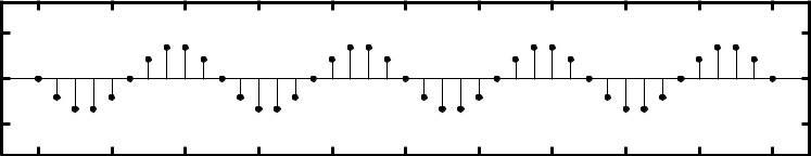
3. xQ3.n/ D si n.0:1 n/ u n/ u.n 10/ Plot 4 periods

%P0203c: x1(n) = {...,-2,-1,0,1,2,-2,-1,0,1,2...}periodic. 5 periods clc; close all;

n3 = [0:11]; x3 = sin(0 1*pi*n3) *(stepseq(0,0,11)-stepseq(10,0,11)); x3 = x3’*ones(1,4); x3 = (x3(:))’; n3 = [-12:35];

Hf_1 = figure; set(Hf 1,’NumberTitle’ , ’off’ , ’Name’ , ’P0203c’); Hs = stem(n3,x3,’filled’);set(Hs,’markersize’,2);axis([min(n3)1,max(n3)+1,min(x3)-0.5,max(x3)+0.5]); xlabel(’n’ , ’FontSize’,LFS); ylabel(’x 3(n)’ , ’FontSize’,LFS); title(’Sequence x_3(n)’ , ’FontSize’,TFS); ntick = [n3(1):4:n3(end)-3 n3(end)];

set(gca,’XTickMode’ , ’manual’ , ’XTick’,ntick); print -deps2 ./CHAP2 EPSFILES/P0203c;

The plots of xQ3.n/ is shown in Figure 2 15

15 SOLUTIONS MANUAL FOR DSP USING MATLAB (4TH EDITION) SOLUTIONS MANUAL FOR DSP USING MATLAB (4TH EDITION) 15 © 2017 Cengage Learning® May not be scanned, copied or duplicated, or posted to a publicly accessible website, in whole or in part © 2017 Cengage Learning® May not be scanned, copied or duplicated, or posted to a publicly accessible website, in whole or in part

1 5 1 0.5 0 SEQUENCE X3(N) −0.5 12 8 4 0 4 8 12 16 20 24 28 32 35 N

Figure 2 15: Problem P2 3 3 sequence plot

24. What is the period of xQ4 n/?

%P0203d x1(n) = {...,-2,-1,0,1,2,-2,-1,0,1,2...}periodic. 5 periods clc; close all;

n4 = [0:24]; x4a = [1 2 3]; x4a = x4a’*ones(1,9); x4a = (x4a(:))’; x4b = [1 2 3

4]; x4b = x4b’*ones(1,7); x4b = (x4b(:))’;

x4 = x4a(1:25) + x4b(1:25);

Hf_1 = figure; set(Hf 1,’NumberTitle’ , ’off’ , ’Name’ , ’P0203d’); Hs = stem(n4,x4,’filled’);set(Hs,’markersize’,2); axis([min(n4)-1,max(n4)+1,min(x4)-1,max(x4)+1]); xlabel(’n’ , ’FontSize’ , LFS); ylabel(’x 4(n)’ , ’FontSize’,LFS); title(’Sequence x 4(n):Period = 12’ , ’FontSize’,TFS);

ntick = [n4(1) :2:n4(end)]; set(gca,’XTickMode’ , ’manual’ , ’XTick’,ntick); print -deps2 ../CHAP2 EPSFILES/P0203d;

The plots of xQ4 n/ is shown in Figure 2 16 From the figure, the fundamental period of xQ4 n/ is 12

16 SOLUTIONS MANUAL FOR DSP USING MATLAB (4TH EDITION) SOLUTIONS MANUAL FOR DSP USING MATLAB (4TH EDITION) 16 © 2017 Cengage Learning® May not be scanned, copied or duplicated, or posted to a publicly accessible website, in whole or in part © 2017 Cengage Learning® May not be scanned, copied or duplicated, or posted to a publicly accessible website, in whole or in part 4 xQ4 n/ D f: : : ; 1; 2; 3; : : :g

C f: : : ; 1; 2; 3; 4; : : :g

; 0

" "

periodic

Sequence x4(n) : Period = 12 8 7 6 5 4 3 2 1 0 2 4 6 8 10 12 14 16 18 20 22 24 n

Figure 2 16: Problem P2 3 4 sequence plot

P2.4 Let x.n/ D f2; 4; 3; 1; 5; 4; 7g. Generate and plot the samples (use the stem function) of the following sequences "

1. x1 .n/ D 2x.n 3/ C 3x n C 4/ x.n/

%P0204a: x(n) = [2,4,-3,1,-5,4,7]; -3 <=n <= 3;

%x1(n) = 2x(n - 3) + 3x(n + 4) - x(n) clc; close all;

n = [-3:3]; x = [2,4,-3,1,-5,4,7];

[x11,n11] = sigshift(x,n,3);

[x12,n12] = sigshift(x,n,-4);

% shift by 3

% shift by -4

[x13,n13] = sigadd(2*x11,n11,3*x12,n12); % add two sequences

[x1,n1] = sigadd(x13,n13,-x,n); % add two sequences

Hf_1 = figure; set(Hf 1,’NumberTitle’ , ’off’ , ’Name’ , ’P0204a’);

Hs = stem(n1,x1,’filled’);set(Hs,’markersize’,2);

axis([min(n1)-1,max(n1)+1,min(x1)-3,max(x1)+1]);

xlabel(’n’ , ’FontSize’,LFS);

ylabel(’x 1(n)’ , ’FontSize’,LFS);

title(’Sequence x 1(n)’ , ’FontSize’,TFS);ntick = n1; ytick = [min(x1)-3:5:max(x1)+1];

set(gca,’XTickMode’ , ’manual’ , ’XTick’,ntick);

set(gca,’YTickMode’ , ’manual’ , ’YTick’,ytick); print -deps2

../CHAP2 EPSFILES/P0204a;

SOLUTIONS MANUAL FOR DSP USING MATLAB (4TH EDITION) 17 17 SOLUTIONS MANUAL FOR DSP USING MATLAB (4TH EDITION)

The plots of x1.n/ is shown in Figure 2.17. 25 20 15 10 5 0 5 −10 15 −20 SEQUENCE X1(N) −7 −6 −5 −4 −3 −2 −1 0 1 2 3 4 5 6 N

Figure 2 17: Problem P2 4 1 sequence plot

2. x2 .n/ D 4x.4 C n/ C 5x.n C 5/ C 2x.n/

%P0204b: x(n) = [2,4,-3,1,-5,4,7]; -3 <=n <= 3;

%x2(n) = 4x(4 + n) + 5x(n + 5) + 2x(n) clc; close all;

Hf_1 = figure; set(Hf 1,’NumberTitle’ , ’off’ , ’Name’ , ’P0204b’); n = [-3:3]; x = [2,4,-3,1,-5,4,7];

[x21,n21] = sigshift(x,n,-4); % shift by -4

[x22,n22] = sigshift(x,n,-5); % shift by -5

[x23,n23] = sigadd(4*x21,n21,5*x22,n22); % add two sequences

[x2,n2] = sigadd(x23,n23,2*x,n); % add two sequences

Hs = stem(n2,x2,’filled’);set(Hs,’markersize’,2);axis([min(n2)1,max(n2)+1,min(x2)-4,max(x2)+6]); xlabel(’n’ , ’FontSize’,LFS); ylabel(’x 2(n)’ , ’FontSize’,LFS); title(’Sequence x_2(n)’ , ’FontSize’,TFS); ntick = n2; ytick = [-25 -20:10:60 65];

set(gca,’XTickMode’ , ’manual’ , ’XTick’,ntick); set(gca,’YTickMode’ , ’manual’ , ’YTick’,ytick); print -deps2 ./CHAP2 EPSFILES/P0204b;

18 SOLUTIONS MANUAL FOR DSP USING MATLAB (4TH EDITION) SOLUTIONS MANUAL FOR DSP USING MATLAB (4TH EDITION) 18 ©

Cengage Learning®. May not be scanned, copied or duplicated, or posted to a publicly accessible website, in whole or in part. © 2017 Cengage Learning® May not be scanned, copied or duplicated, or posted to a publicly accessible website, in whole or in part

2017

The

2.n/

65 60 50 40 30 20 10 0 −10 20 −25 SEQUENCE X2(N) −8 −7 −6 −5 −4 −3 −2 −1 0 1 2 3 N

plots of x

is shown in Figure 2.18.

Figure 2 18: Problem P2 4 2 sequence plot

%P0204c: x(n) = [2,4,-3,1,-5,4,7]; -3 <=n <= 3;

% x3(n) = x(n + 3)x(n - 2) + x(1 - n)x(n + 1) clc; close all;

n = [-3:3]; x = [2,4,-3,1,-5,4,7]; % given sequence x(n)

[x31,n31] = sigshift(x,n,-3);

[x32,n32] = sigshift(x,n,2);

% shift sequence by -3

% shift sequence by 2

[x33,n33] = sigmult(x31,n31,x32,n32); % multiply 2 sequences

[x34,n34] = sigfold(x,n); % fold x(n)

[x34,n34] = sigshift(x34,n34,1);

% shift x(-n) by 1

[x35,n35] = sigshift(x,n,-1); % shift x(n) by -1

[x36,n36] = sigmult(x34,n34,x35,n35); % multiply 2 sequences

[x3,n3] = sigadd(x33,n33,x36,n36); % add 2 sequences

Hf_1 = figure; set(Hf 1,’NumberTitle’ , ’off’ , ’Name’ , ’P0204c’); Hs = stem(n3,x3,’filled’);set(Hs,’markersize’,2);axis([min(n3)1,max(n3)+1,min(x3)-10,max(x3)+10]); xlabel(’n’ , ’FontSize’,LFS); ylabel(’x 3(n)’ , ’FontSize’,LFS); title(’Sequence x_3(n)’ , ’FontSize’,TFS); ntick = n3; ytick = [-30:10:60];

set(gca,’XTickMode’ , ’manual’ , ’XTick’,ntick); set(gca,’YTickMode’ , ’manual’ , ’YTick’,ytick); print -deps2 ./CHAP2 EPSFILES/P0204c;

19 SOLUTIONS MANUAL FOR DSP USING MATLAB (4TH EDITION) SOLUTIONS MANUAL FOR DSP USING MATLAB (4TH EDITION) 19 © 2017 Cengage Learning®. May not be scanned, copied or duplicated, or posted to a publicly accessible website, in whole or in part. © 2017 Cengage Learning® May not be scanned, copied or duplicated, or posted to a publicly accessible website, in whole or in part 3. x3 .n/ D x.n C 3/x.n 2/ C x.1 n/x.n C 1/

The plots of x3.n/ is shown in Figure 2.19. 60 50 40 30 20 10 0 10 20 −30 SEQUENCE X3(N) 6 5 4 3 2 1 0 1 2 3 4 5 N

Figure 2 19: Problem P2 4 3 sequence plot

%P0204d: x(n) = [2,4,-3,1,-5,4,7]; -3 <=n <= 3;

% x4(n) = 2*e^{0 5n}*x(n)+cos(0.1*pi*n)*x(n+2), -10 <=n< =10 clc; close all;

n = [-3:3]; x = [2,4,-3,1,-5,4,7];

% given sequence x(n)

n4 = [-10:10]; x41 = 2*exp(0.5*n4); x412 = cos(0.1*pi*n4);

[x42,n42] = sigmult(x41,n4,x,n);

[x43,n43] = sigshift(x,n,-2);

[x44,n44] = sigmult(x412,n42,x43,n43);

[x4,n4] = sigadd(x42,n42,x44,n44);

Hf_1 = figure; set(Hf 1,’NumberTitle’ , ’off’ , ’Name’ , ’P0204d’); Hs = stem(n4,x4,’filled’);set(Hs,’markersize’,2);axis([min(n4)1,max(n4)+1,min(x4)-11,max(x4)+10]); xlabel(’n’ , ’FontSize’,LFS); ylabel(’x 4(n)’ , ’FontSize’,LFS); title(’Sequence x_4(n)’ , ’FontSize’,TFS); ntick = n4; ytick = [ -20:10:70];

set(gca,’XTickMode’ , ’manual’ , ’XTick’,ntick); set(gca,’YTickMode’ , ’manual’ , ’YTick’,ytick); print -deps2 ./CHAP2 EPSFILES/P0204d; The

shown in Figure 2 20

20 SOLUTIONS MANUAL FOR DSP USING MATLAB (4TH EDITION) SOLUTIONS MANUAL FOR DSP USING MATLAB (4TH EDITION) 20 © 2017 Cengage Learning®. May not be scanned, copied or duplicated, or posted to a publicly accessible website, in whole or in part. © 2017 Cengage Learning® May not be scanned, copied or duplicated, or posted to a publicly accessible website, in whole or in part 4. x4 .n/ D 2e 0:5n x .n/ C cos .0:1 n/ x .n C 2/ ; 10 n 10

of x4.n/

70 60 50 40 30 20 10 0 10 20 SEQUENCE X4(N) 10 9 8 7 6 5 4 3 2 1 0 1 2 3 4 5 6 7 8 9 10 N

plot

Figure 2.20: Problem P2.4.4 sequence plot

The complex exponential sequence

the sinusoidal sequence cos

are periodic if the normalized frequency

f0 D 2 is a rational number; thatis, f0 DN , where K and N are integers.

1.Analytical proof: The exponential sequence is periodic if

which proves the result.

2.x1 D exp.0:1 n/; 100 n 100.

%P0205b: x1(n) = e^{0 1*j*pi*n} -100 <=n <=100 clc; close all; n1 = [-100:100]; x1 = exp(0.1*j*pi*n1); Hf_1 = figure; set(Hf 1,’NumberTitle’ , ’off’ , ’Name’ , ’P0205b’); subplot(2,1,1); Hs1 = stem(n1,real(x1),’filled’);set(Hs1,’markersize’,2);axis([min(n1)5,max(n1)+5,min(real(x1))-1,max(real(x1))+1]); xlabel(’n’ , ’FontSize’,LFS); ylabel(’Real(x 1(n))’ , ’FontSize’,LFS); title([’Real part of sequence x_1(n) = ’ ...

’exp(0.1 \times j \times pi \times n) ’ char(10)

’ Period = 20, K = 1, N = 20’],’FontSize’,TFS);

ntick = [n1(1):20:n1(end)]; set(gca,’XTickMode’ , ’manual’ , ’XTick’,ntick); subplot(2,1,2); Hs2 = stem(n1,imag(x1),’filled’);set(Hs2,’markersize’,2);axis([min(n1)5,max(n1)+5,min(real(x1))-1,max(real(x1))+1]); xlabel(’n’ , ’FontSize’,LFS); ylabel(’Imag(x 1(n))’ , ’FontSize’,LFS); title([’Imaginarypart of sequence x_1(n) = ’ ...

’exp(0.1 \times j \times pi \times n) ’ char(10)

’ Period = 20, K = 1, N = 20’],’FontSize’,TFS); ntick = [n1(1):20:n1(end)]; set(gca,’XTickMode’ , ’manual’ , ’XTick’,ntick); print -deps2 ../CHAP2 EPSFILES/P0205b; print -deps2 ../../Latex/P0205b;

The plots of x1.n/ is shown in Figure 2.21. Since f0 D 0:1=2 D 1=20 the sequence is periodic. From the plot in Figure 2 21 we see that in one period of 20 samples x1 .n/ exhibits cycle. This is true whenever K and N are relatively prime.

3. x2 D cos.0:1n/; 20 n 20

%P0205c: x2(n) = cos(0.1n), -20 <= n <= 20 clc; close all;

n2 = [-20:20]; x2 = cos(0.1*n2);

Hf_1 = figure; set(Hf 1,’NumberTitle’ , ’off’ , ’Name’ , ’P0205c’); Hs = stem(n2,x2,’filled’);set(Hs,’markersize’,2);axis([min(n2)1,max(n2)+1,min(x2)-1,max(x2)+1]); xlabel(’n’ , ’FontSize’,LFS); ylabel(’x 2(n)’ , ’FontSize’,LFS); title([’Sequence x 2(n) = cos(0.1 \times n)’ char(10)

’Not periodic since f_0 = 0 1 / (2 \times \pi)’

’ is not a rational number’], ’FontSize’,TFS);

ntick = [n2(1):4:n2(end)]; set(gca,’XTickMode’ , ’manual’ , ’XTick’,ntick); print -deps2

../CHAP2 EPSFILES/P0205c;

The plots of x1.n/ is shown in Figure 2.22. In this case f0 is not a rational number and hence the sequence x2 .n/ is not periodic This can be clearly seen from the plot of x2 .n/ in Figure 2.22.

21 SOLUTIONS MANUAL FOR DSP USING MATLAB (4TH EDITION) SOLUTIONS MANUAL FOR DSP USING MATLAB (4TH EDITION) 21 © 2017 Cengage Learning®. May not be scanned, copied or duplicated, or posted to a publicly accessible website, in whole or in part. © 2017 Cengage Learning® May not be scanned, copied or duplicated, or posted to a publicly accessible website, in whole or in part e 0 P2.5

j! n 4 !0 or

j 2 f nCN/ 0 j 2 f n De 0 ore j 2 f N 0 D1)f0NDK(an

integer)

22 SOLUTIONS MANUAL FOR DSP USING MATLAB (4TH EDITION) SOLUTIONS MANUAL FOR DSP USING MATLAB (4TH EDITION) 22 © 2017 Cengage Learning®. May not be scanned, copied or duplicated, or posted to a publicly accessible website, in whole or in part. © 2017 Cengage Learning® May not be scanned, copied or duplicated, or posted to a publicly accessible website, in whole or in part Sequence x2(n) = cos(0.1 × n) Not periodic since f0 = 0.1 / (2 × π) is not a rational number 2 1.5 1 0 5 0 −0.5 1 20 16 12 8 4 0 4 8 12 16 20 n

2 1 5 1 0 5 0 −0.5 −1 −20 −16 −12 −8 −4 0 4 8 12 16 20 n

Figure 2.21:

Problem P2.5.2 sequence plots

Sequence x2(n) = cos(0.1 × n) Not periodic since f0 = 0.1 / (2 ×

) is not a rational number

Figure 2.22: Problem P2.5 3 sequence plots

P2.6 Using the evenodd function decompose the following sequences into their even and odd components. Plot these compo-nents using the stem function

1. x1.n/ D f0; 1; 2; 3; 4; 5; 6; 7; 8; 9g. "

% P0206a: % Even odd decomposition of x1(n) = [0 1 2 3 4 5 6 7 8 9];

% n = 0:9; clc; close all;

x1 = [0 1 2 3 4 5 6 7 8 9]; n1 = [0:9]; [xe1,xo1,m1] = evenodd(x1,n1);

Hf_1 = figure; set(Hf 1,’NumberTitle’ , ’off’ , ’Name’ , ’P0206a’); subplot(2,1,1); Hs

= stem(m1,xe1,’filled’);set(Hs,’markersize’,2);axis([min(m1)1,max(m1)+1,min(xe1)-1,max(xe1)+1]); xlabel(’n’ , ’FontSize’,LFS); ylabel(’x e(n)’ , ’FontSize’,LFS); title(’Even part of x 1(n)’ , ’FontSize’,TFS);ntick = [m1(1):m1(end)]; ytick = [-1:5];

set(gca,’XTick’,ntick);set(gca,’YTick’,ytick); subplot(2,1,2); Hs = stem(m1,xo1,’filled’);set(Hs,’markersize’,2); axis([min(m1)-1,max(m1)+1,min(xo1)-2,max(xo1)+2]); xlabel(’n’ , ’FontSize’,LFS);ylabel(’x o(n)’ , ’FontSize’,LFS); title(’Odd part of x 1(n)’ , ’FontSize’,TFS);ntick = [m1(1):m1(end)]; ytick = [-6:2:6];

set(gca,’XTick’,ntick);set(gca,’YTick’,ytick); print -deps2 ./CHAP2 EPSFILES/P0206a; print -deps2 ./. /Latex/P0206a;

23 SOLUTIONS MANUAL FOR DSP USING MATLAB (4TH EDITION) SOLUTIONS MANUAL FOR DSP USING MATLAB (4TH EDITION) 23 © 2017 Cengage Learning®. May not be scanned, copied or duplicated, or posted to a publicly accessible website, in whole or in part. © 2017 Cengage Learning® May not be scanned, copied or duplicated, or posted to a publicly accessible website, in whole or in part

The plots of x1.n/ is shown in Figure 2.23. Even part of x1(n) 5 4 3 2 1 0 −1 9 8 7 6 5 4 3 2 1 0 1 2 3 4 5 6 7 8 9 n Odd part of x1(n) 6 4 2 0 −2 −4 −6 9 8 7 6 5 4 3 2 1 0 1 2 3 4 5 6 7 8 9 n

Figure 2 23: Problem P2 6 1 sequence plot

%P0206b: Even odd decomposition of x2(n) = e ^ {0.1n} [u(n + 5) - u(n - 10)]; clc; close all;

n2 = [-8:12]; x2 = exp(0.1*n2).*(stepseq(-5,-8,12) - stepseq(10,-8,12));[xe2,xo2,m2] = evenodd(x2,n2);

Hf_1 = figure; set(Hf 1,’NumberTitle’ , ’off’ , ’Name’ , ’P0206b’); subplot(2,1,1); Hs = stem(m2,xe2,’filled’);set(Hs,’markersize’,2);axis([min(m2)1,max(m2)+1,min(xe2)-1,max(xe2)+1]); xlabel(’n’ , ’FontSize’,LFS); ylabel(’x e(n)’ , ’FontSize’,LFS); title(’Even part of x 2(n) = exp(0.1n) [u(n + 5)u(n - 10)]’ ,...

’FontSize’,TFS); ntick = [m2(1):2:m2(end)];set(gca,’XTick’,ntick); subplot(2,1,2); Hs = stem(m2,xo2,’filled’);set(Hs,’markersize’,2); axis([min(m2)-1,max(m2)+1,min(xo2)-1,max(xo2)+1]); xlabel(’n’ , ’FontSize’,LFS);ylabel(’x o(n)’ , ’FontSize’,LFS); title(’Odd part of x 2(n) = exp(0.1n) [u(n + 5) - u(n - 10)]’ ,...

’FontSize’,TFS);

ntick = [m2(1) :2:m2(end)]; set(gca,’XTick’,ntick); print -deps2 ./CHAP2 EPSFILES/P0206b; print -deps2 ./. /Latex/P0206b;

The plots of x2.n/ is shown in Figure 2.24.

24 SOLUTIONS MANUAL FOR DSP USING MATLAB (4TH EDITION) SOLUTIONS MANUAL FOR DSP USING MATLAB (4TH EDITION) 24 © 2017 Cengage Learning®. May not be scanned, copied or duplicated, or posted to a publicly accessible website, in whole or in part. © 2017 Cengage Learning® May not be scanned, copied or duplicated, or posted to a publicly accessible website, in whole or in part 0:1n 2. x2.n/ D e u.n C 5/ u.n 10/

Even part of x2(n) = exp(0.1n) [u(n + 5) − u(n − 10)] 2 1 0 −1 12 10 8 6 4 2 0 2 4 6 8 10 12 n Odd part of x2(n) = exp(0.1n) [u(n + 5) − u(n − 10)] 2 0 2 12 10 8 6 4 2 0 2 4 6 8 10 12 n

Figure 24: Problem P2 6 2 sequence plot

3. x3.n/ D cos 0:2 n C =4/; 20 n 20

% P0206c: Even odd decomposition of x2(n) = cos(0.2*pi*n + pi/4);

% -20 <= n <= 20; clc; close all;

n3 = [-20:20]; x3 = cos(0.2*pi*n3 + pi/4); [xe3,xo3,m3] = evenodd(x3,n3);

Hf_1 = figure; set(Hf 1,’NumberTitle’ , ’off’ , ’Name’ , ’P0206c’); subplot(2,1,1); Hs = stem(m3,xe3,’filled’);set(Hs,’markersize’,2);axis([min(m3)-2,max(m3)+2,min(xe3)1,max(xe3)+1]); xlabel(’n’ , ’FontSize’,LFS);ylabel(’x_e(n)’ , ’FontSize’,LFS); title(’Even part of x 3(n) = cos(0.2 \times \pi \times n + \pi/4)’ ,...

’FontSize’,TFS);

ntick = [m3(1):4:m3(end)];set(gca,’XTick’,ntick); subplot(2,1,2); Hs = stem(m3,xo3,’filled’);set(Hs,’markersize’,2);axis([min(m3)2,max(m3)+2,min(xo3)-1,max(xo3)+1]); xlabel(’n’ , ’FontSize’,LFS); ylabel(’x o(n)’ , ’FontSize’,LFS); title(’Odd part of x 3(n) = cos(0.2 \times \pi \times n + \pi/4)’ ,...

’FontSize’,TFS);

ntick = [m3(1):4 :m3(end)]; set(gca,’XTick’,ntick); print -deps2 ./CHAP2 EPSFILES/P0206c; print -deps2 ./. /Latex/P0206c;

The plots of x3.n/ is shown in Figure 2.25.

25 SOLUTIONS MANUAL FOR DSP USING MATLAB (4TH EDITION) SOLUTIONS MANUAL FOR DSP USING MATLAB (4TH EDITION) 25 © 2017 Cengage Learning®. May not be scanned, copied or duplicated, or posted to a publicly accessible website, in whole or in part. © 2017 Cengage Learning® May not be scanned, copied or duplicated, or posted to a publicly accessible website, in whole or in part

Even part of x3(n) = cos(0.2 × π × n + π/4) 1 0 −1 20 16 12 8 4 0 4 8 12 16 20 n Odd part of x3(n) = cos(0.2 × π × n + π/4) 1 0 −1 −20 −16 −12 −8 −4 0 4 8 12 16 20 n

Figure 2 25: Problem P2 6 3 sequence plot

0:05n 4. x4.n/ D e sin.0:1 n C =3/; 0 n 100

%P0206d: x4(n) = e ^ {-0 05*n}*sin(0 1*pi*n+ pi/3), 0 <= n <= 100 clc; close all;

n4 = [0:100]; x4 = exp(-0.05*n4) *sin(0.1*pi*n4 + pi/3); [xe4,xo4,m4] = evenodd(x4,n4);

Hf_1 = figure; set(Hf 1,’NumberTitle’ , ’off’ , ’Name’ , ’P0206d’); subplot(2,1,1); Hs = stem(m4,xe4,’filled’);set(Hs,’markersize’,2);axis([min(m4)10,max(m4)+10,min(xe4)-1,max(xe4)+1]); xlabel(’n’ , ’FontSize’,LFS); ylabel(’x e(n)’ , ’FontSize’,LFS); title([’Even part of x 4(n) = ’

’exp(-0.05 \times n) \times sin(0.1 \times \pi \times n + ’ ...

’\pi/3)’],’FontSize’,TFS);

ntick = [m4(1):20:m4(end)];set(gca,’XTick’,ntick);

subplot(2,1,2); Hs = stem(m4,xo4,’filled’);set(Hs,’markersize’,2); axis([min(m4)-10,max(m4)+10,min(xo4)-1,max(xo4)+1]); xlabel(

’n’ , ’FontSize’,LFS);ylabel(’x o(n)’ , ’FontSize’,LFS); title([’Odd part of x 4(n) = ’

’exp(-0.05 \times n) \times sin(0.1 \times \pi \times n + ’ ’\pi/3)’],’FontSize’,TFS); ntick = [m4(1):20 :m4(end)]; set(gca,’XTick’,ntick); print -deps2 ./CHAP2 EPSFILES/P0206d; print -deps2 ./. /Latex/P0206d; The plots of x1.n/ are shown in Figure 2 26

26 SOLUTIONS MANUAL FOR DSP USING MATLAB (4TH EDITION) SOLUTIONS MANUAL FOR DSP USING MATLAB (4TH EDITION) 26 © 2017 Cengage Learning®. May not be scanned, copied or duplicated, or posted to a publicly accessible website, in whole or in part. © 2017 Cengage Learning® May not be scanned, copied or duplicated, or posted to a publicly accessible website, in whole or in part

Even part of x4(n) = exp(−0.05 × n) × sin(0.1 × π × n + π/3) 1 0 1 100 80 60 40 20 0 20 40 60 80 100 n Odd part of x4(n) = exp(−0.05 × n) × sin(0.1 × π × n + π/3) 1 0 −1 100 80 60 40 20 0 20 40 60 80 100 n

Figure 2.26: Problem P2.6.1 sequence plot

P2 7 A complex-valued sequence xe n/ is called conjugate-symmetric if xe.n/ D xe n/ and a complex-valued sequence xo n/ is called conjugate-antisymmetric if xo n/ x n/ Then anyarbitrary complex-valued sequencex.n/ can be o decomposed into x.n/ D xe.n/ C xo.n/ where xe.n/ and xo.n/ are given by

1. Modify the evenodd function discussed in the text so that it accepts an arbitrary sequence and decomposes it into its conjugate-symmetricand conjugate-antisymmetriccomponents by implementing (2.1).

function [xe , xo , m] = evenodd c(x , n)

%Complex-valued signal decomposition into even and odd parts (version-2)

% - - - - - - - --- - - - - - - - --

%[xe , xo , m] = evenodd c(x , n);

% [xc , nc] = sigfold(conj(x) , n);

[xe , m] = sigadd(0.5 * x , n , 0.5 * xc , nc);

[xo , m] = sigadd(0.5 * x , n , -0.5 * xc , nc);

2. x.n/ D 10 exp. 0:1 C | 0:2 n/; 0 n 10

% P0207b: Decomposition of x(n) = 10*e ^ {(-0.1 + j*0 2*pi)*n},

% 0 < = n <= 10

%into its conjugate symmetric and conjugate antisymmetric parts. clc; close all;

n = [0:10]; x = 10*exp((-0.1+j*0.2*pi)*n);[xe,xo,neo] = evenodd(x,n); Re xe = real(xe); Im xe = imag(xe); Re_xo = real(xo); Im xo = imag(xo);

Hf_1 = figure; set(Hf 1,’NumberTitle’ , ’off’ , ’Name’ , ’P0207b’); subplot(2,2,1); Hs = stem(neo,Re xe); set(Hs,’markersize’,2); ylabel(’Re[x_e(n)]’ , ’FontSize’,LFS); xlabel(’n’ , ’FontSize’,LFS); axis([min(neo)-1,max(neo)+1,-5,12]); ytick = [-5:5:15]; set(gca,’YTick’,ytick);

title([’Real part of’ char(10) ’even sequence x e(n)’],’FontSize’,TFS);

subplot(2,2,3); Hs = stem(neo,Im xe);set(Hs,’markersize’,2); ylabel(’Im[x e(n)]’ , ’FontSize’,LFS); xlabel(’n’ , ’FontSize’,LFS); axis([min(neo)-1,max(neo)+1,-5,5]); ytick = [-5:1:5]; set(gca,’YTick’,ytick);

title([’Imaginarypart of’ char(10) ’even sequence x_e(n)’],’FontSize’,TFS);

subplot(2,2,2); Hs = stem(neo,Re xo);set(Hs,’markersize’,2); ylabel(’Re[x_o(n)]’ , ’FontSize’,LFS); xlabel(’n’ , ’FontSize’,LFS); axis([min(neo)-1,max(neo)+1,-5,+5]); ytick = [-5:1:5]; set(gca,’YTick’,ytick);

title([’Real part of’ char(10) ’odd sequence x o(n)’],’FontSize’,TFS);

subplot(2,2,4); Hs = stem(neo,Im xo);set(Hs,’markersize’,2); ylabel(’Im[x o(n)]’ , ’FontSize’,LFS); xlabel(’n’ , ’FontSize’,LFS); axis([min(neo)-1,max(neo)+1,-5,5]); ytick = [-5:1:5]; set(gca,’YTick’,ytick);

title([’Imaginarypart of’ char(10) ’odd sequence x o(n)’],’FontSize’,TFS);print -deps2 ../EPSFILES/P0207b;%print -deps2 ./. /Latex/P0207b; The plots of x.n/ are shown in Figure 2 27.

27 SOLUTIONS MANUAL FOR DSP USING MATLAB (4TH EDITION) SOLUTIONS MANUAL FOR DSP USING MATLAB (4TH EDITION) 27 © 2017 Cengage Learning®. May not be scanned, copied or duplicated, or posted to a publicly accessible website, in whole or in part. © 2017 Cengage Learning® May not be scanned, copied or duplicated, or posted to a publicly accessible website, in whole or in part D

1 1 respectively xe.n/ D 2 x.n/ C x .n/ and xo.n/ D 2 x.n/ x n/ (2.1)

28 SOLUTIONS MANUAL FOR DSP USING MATLAB (4TH EDITION) SOLUTIONS MANUAL FOR DSP USING MATLAB (4TH EDITION) 28 © 2017 Cengage Learning®. May not be scanned, copied or duplicated, or posted to a publicly accessible website, in whole or in part. © 2017 Cengage Learning® May not be scanned, copied or duplicated, or posted to a publicly accessible website, in whole or in part ) ] ) ] Real part of Real part of even sequence xe(n) odd sequence xo(n) 5 10 4 5 3 2 0 0 1 −3 4 5 5 10 5 0 5 10 10 5 0 5 10 n n Imaginary part of Imaginary part of even sequence xe(n) odd sequence xo(n) 5 5 4 4 3 3 2 2 0 0 −1 −1 −3 −3 4 4 5 5 10 5 0 5 10 10 5 0 5 10 n n

Figure 2.27: Problem P2.7 2 sequence plot

P2.8 The operation of signal dilation (or decimation or down-sampling) is defined by y n/ D x nM / in which the sequence x.n/ is down-sampled by an integer factor M .

1. MATLAB function:

function [y,m] = dnsample(x,n,M)

%[y,m] = dnsample(x,n,M)

%Downsample sequence x(n) by a factor M to obtain y(m) mb = ceil(n(1)/M)*M; me = floor(n(end)/M)*M;

nb = find(n==mb); ne = find(n==me);

y = x(nb:M:ne); m = fix((mb:M:me)/M);

2. x1.n/ D sin.0:125 n/; 50 n 50 Decimation by a factor of 4

%P0208b: x1(n) = sin(0 125*pi*n),-50<= n <= 50

% Decimate x(n) by a factor of 4 to obtain y(n) clc; close all;

n1 = [-50:50]; x1 = sin(0.125*pi*n1); [y1,m1] = dnsample(x1,n1,4);Hf_1 = figure; set(Hf 1,’NumberTitle’ , ’off’ , ’Name’ , ’P0208b’); subplot(2,1,1); Hs = stem(n1,x1); set(Hs,’markersize’,2);xlabel(’n’ , ’FontSize’,LFS); ylabel(’x(n)’ , ’FontSize’,LFS); title(’Original sequence x 1(n)’ , ’FontSize’,TFS); axis([min(n1)-5,max(n1)+5,min(x1)-0.5,max(x1)+0.5]);

ytick = [-1.5:0.5:1.5]; ntick = [n1(1):10:n1(end)]; set(gca,’XTick’,ntick); set(gca,’YTick’,ytick);subplot(2,1,2); Hs = stem(m1,y1); set(Hs,’markersize’,2);xlabel(’n’ , ’FontSize’,LFS); ylabel(’y(n) = x(4n)’ , ’FontSize’,LFS);

title(’y 1(n) = Original sequence x 1(n) decimated by a factor of 4’ ,...

’FontSize’,TFS); axis([min(m1)-2,max(m1)+2,min(y1)0.5,max(y1)+0.5]); ytick = [-1.5:0.5:1.5]; ntick = [m1(1):2:m1(end)];set(gca,’XTick’,ntick); set(gca,’YTick’,ytick);print -deps2

../CHAP2 EPSFILES/P0208b;

The plots of x1 n/ and y1 n/ are shown in Figure 2 28 Observe that the original signal x1 n/ can be recovered

3. x.n/ D sin 0:5 n/; 50 n 50 Decimation by a factor of 4

%P0208c: x2(n) = sin(0.5*pi*n),-50 <= n <= 50

% Decimate x2(n) by a factor of 4 to obtain y2(n) clc; close all;

n2 = [-50:50]; x2 = sin(0.5*pi*n2); [y2,m2] = dnsample(x2,n2,4); Hf_1 = figure; set(Hf 1,’NumberTitle’ , ’off’ , ’Name’ , ’P0208c’); subplot(2,1,1); Hs = stem(n2,x2); set(Hs,’markersize’,2);xlabel(’n’ , ’FontSize’,LFS); ylabel(’x(n)’ , ’FontSize’,LFS); axis([min(n2)-5,max(n2)+5,min(x2)0.5,max(x2)+0.5]);title(’Original sequence x_2(n)’ , ’FontSize’,TFS);

ytick = [-1.5:0 5:1 5]; ntick = [n2(1):10:n2(end)]; set(gca,’XTick’,ntick); set(gca,’YTick’,ytick);subplot(2,1,2); Hs = stem(m2,y2); set(Hs,’markersize’,2);xlabel(’n’ , ’FontSize’,LFS); ylabel(’y(n) = x(4n)’ , ’FontSize’,LFS);axis([min(m2)-1,max(m2)+1,min(y2)-1,max(y2)+1]);

title(’y 2(n) = Original sequence x_2(n) decimated by a factor of 4’ ,...

’FontSize’,TFS);

ntick = [m2(1):2:m2(end)];set(gca,’XTick’,ntick); print -deps2 ./CHAP2 EPSFILES/P0208c; print -deps2 ./. /Latex/P0208c;

29 SOLUTIONS MANUAL FOR DSP USING MATLAB (4TH EDITION) SOLUTIONS MANUAL FOR DSP USING MATLAB (4TH EDITION) 29 © 2017 Cengage Learning®. May not be scanned, copied or duplicated, or posted to a publicly accessible website, in whole or in part. © 2017 Cengage Learning® May not be scanned, copied or duplicated, or posted to a publicly accessible website, in whole or in part

The plots of x2.n/ and y2.n/ are shown in Figure 2.29. Observe that the downsampled signal is a signal with zero frequency. Thus the original signal x2.n/ is lost.

30 SOLUTIONS MANUAL FOR DSP USING MATLAB (4TH EDITION) SOLUTIONS MANUAL FOR DSP USING MATLAB (4TH EDITION) 30 © 2017 Cengage Learning®. May not be scanned, copied or duplicated, or posted to a publicly accessible website, in whole or in part. © 2017 Cengage Learning® May not be scanned, copied or duplicated, or posted to a publicly accessible website, in whole or in part 1 5 1 0 5 0 0 5 1 1 5 Original sequence x1(n) −50 −40 −30 −20 −10 0 10 20 30 40 50 n y1(n) = Original sequence x1(n) decimated by a factor of 4 1 5 1 0.5 0 −0 5 −1 1 5 12 10 8 6 4 2 0 2 4 6 8 10 12 n

1 5 1 0 5 0 −0 5 1 1 5 Original sequence x2(n) −50 −40 −30 −20 −10 0 10 20 30 40 50 n y2(n) = Original sequence x2(n) decimated by a factor of 4 1 0 −1 12 10 8 6 4 2 0 2 4 6 8 10 12 n

Figure 2 28: Problem P2 8 2 sequence plot Figure 2.29: Problem P2.8 3 sequence plot

P2.9 The autocorrelation sequence rxx ‘/ and the crosscorrelation sequence rxy ‘/ for the sequences:

%P0209a: autocorrelation of sequence x(n) = 0.9 ^ n, 0 <= n <= 20 %using the conv_m function clc; close all;

nx = [0:20]; x = 0.9 . ^ nx; [xf,nxf] = sigfold(x,nx); [rxx,nrxx] = conv m(x,nx,xf,nxf);

Hf_1 = figure; set(Hf 1,’NumberTitle’ , ’off’ , ’Name’ , ’P0209a’); Hs = stem(nrxx,rxx); set(Hs,’markersize’,2);xlabel(’n’ , ’FontSize’,LFS); ylabel(’r x x(n)’ , ’FontSize’,LFS); title(’Autocorrelation of x(n)’ , ’FontSize’,TFS);axis([min(nrxx)1,max(nrxx)+1,min(rxx),max(rxx)+1]);

ntick = [nrxx(1):4:nrxx(end)];set(gca,’XTick’,ntick);%printdeps2 ./CHAP2 EPSFILES/P0209a;

The plot of the autocorrelation is shown in Figure 2.30.

AUTOCORRELATION OF X(N)

%P0209b: crosscorrelation of sequence x(n) = 0.9 ^ n, 0 <= n <= 20

% with sequence y = 0 8.^n, -20 <=n <= 0 using the conv_m function clc; close all;

nx = [0:20]; x = 0.9 . ^ nx; ny = [-20:0]; y = 0.8 . ^ (-ny); [yf,nyf] = sigfold(y,ny); [rxy,nrxy] = conv m(x,nx,yf,nyf);

Hf_1 = figure; set(Hf 1,’NumberTitle’ , ’off’ , ’Name’ , ’P0209b’); Hs = stem(nrxy,rxy); set(Hs,’markersize’,3);xlabel(’n’ , ’FontSize’,LFS);

31 SOLUTIONS MANUAL FOR DSP USING MATLAB (4TH EDITION) SOLUTIONS MANUAL FOR DSP USING MATLAB (4TH EDITION) 31 © 2017 Cengage Learning®. May not be scanned, copied or duplicated, or posted to a publicly accessible website, in whole or in part. © 2017 Cengage Learning® May not be scanned, copied or duplicated, or posted to a publicly accessible website, in whole or in part

n x.n/ D .0:9/ n ; 0 n 20I y n/ D .0:8/ ; 20 n 0

6 5 4 3 2 1 20 16 12 8 4 0 4 8 12 16 20 N

Figure 2.30: Problem P2.9 autocorrelation plot

ylabel(’r x y(n)’ , ’FontSize’,LFS); title(’Crosscorrelation of x(n) and y(n)’ , ’FontSize’,TFS);

32 SOLUTIONS MANUAL FOR DSP USING MATLAB (4TH EDITION) SOLUTIONS MANUAL FOR DSP USING MATLAB (4TH EDITION) 32 © 2017 Cengage Learning®. May not be scanned, copied or duplicated, or posted to a publicly accessible website, in whole or in part. © 2017 Cengage Learning® May not be scanned, copied or duplicated, or posted to a publicly accessible website, in whole or in part

axis([min(nrxy)-1,max(nrxy)+1,floor(min(rxy)),ceil(max(rxy))]); ytick = [0:1:4]; ntick = [nrxy(1):2:nrxy(end)];set(gca,’XTick’,ntick); set(gca,’YTick’,ytick);print -deps2 ./epsfiles/P0209b;

The plot of the crosscorrelation is shown in Figure 2.31

33 SOLUTIONS MANUAL FOR DSP USING MATLAB (4TH EDITION) SOLUTIONS MANUAL FOR DSP USING MATLAB (4TH EDITION) 33 © 2017 Cengage Learning®. May not be scanned, copied or duplicated, or posted to a publicly accessible website, in whole or in part. © 2017 Cengage Learning® May not be scanned, copied or duplicated, or posted to a publicly accessible website, in whole or in part

3 2 1 0 0 2 4 6 8 10 12 14 16 18 20 22 24 26 28 30 32 34 36 38 40 n

Crosscorrelation of x(n) and y(n)

Figure 2.31: Problem P2.9 crosscorrelation plot

P2.10 In a certain concert hall, echoes of the original audio signal x.n/ are generated due to the reflections at the walls and ceiling The audio signal experienced by the listener y n/ is a combination of x.n/ and its echoes Let y n/ D x n/ C x.n k/ where k is the amount of delay in samples and is its relative strength. We want to estimate the delay using the correlation analysis.

1. Determine analyticallythe autocorrelation ryy ‘/ in terms of the autocorrelation rxx ‘/. Consider the autocorrelation ryy ‘/ of y n/:

2. Let x.n/ D cos.0:2 n/ C 0:5 cos.0:6 n/, D 0:1, and k D 50. Generate 200 samples of y.n/ and determine its autocorrelation. Can you obtain and k by observing ryy . ‘/?

MATLAB script:

% P0210c: autocorrelation of sequence y(n) = x(n) + alpha*x(n - k)

% alpha = 0.1,k = 50

%x(n) = cos(0.2*pi*n) + 0 5*cos(0.6*pi*n) clc; close all;

Hf_1 = figure;

set(Hf 1,’NumberTitle’ , ’off’ , ’Name’ , ’P0210c’); alpha = .1;

n = [-100:100];

%x = 3*rand(1,201)-1.5;

x = cos(0.2*pi*n) + 0.5*cos(0.6*pi*n); [xf,nxf]

= sigfold(x,n);

[rxx,nrxx] = conv m(x,n,xf,nxf);

y = filter([1 zeros(1,49) alpha], 1, x);

[yf,nyf] = sigfold(y,n);

[ryx,nryx] = conv m(y,n,xf,nxf);

[ryy,nryy] = conv m(y,n,yf,nyf);

subplot(2,1,1);

Hs = stem(nrxx,rxx,’filled’);

set(Hs,’markersize’,2);

xlabel(’n’ , ’FontSize’,LFS);

ylabel(’r y y(n)’ , ’FontSize’,LFS);

title(’autocorrelation of sequence x(n)’ , ’FontSize’,TFS);

axis([-210, 210,-200,200]);

ntick = [-200:50:200]; ytick = [-200:50:200];

set(gca,’XTickMode’ , ’manual’ , ’XTick’,ntick);

set(gca,’YTickMode’ , ’manual’ , ’YTick’,ytick);

34 SOLUTIONS MANUAL FOR DSP USING MATLAB (4TH EDITION) SOLUTIONS MANUAL FOR DSP USING MATLAB (4TH EDITION) 34 © 2017 Cengage Learning®. May not be scanned, copied or duplicated, or posted to a publicly accessible website, in whole or in part. © 2017 Cengage Learning® May not be scanned, copied or duplicated, or posted to a publicly accessible website, in whole or in part

ryy ‘/ D X‘ y.n/y.n ‘/ D X‘ x.n/ C x.n k/ x.n ‘/ C x.n k ‘/ X D ‘ x.n/x.n ‘/C 2X X ‘ x.n/x.n k ‘/C X ‘ x.n k/x.n ‘/ C ‘ x.n k/x.n k ‘/ 2 D rxx. ‘/ C rxx.‘ C k/ C rxx.‘ k/ C rxx.‘/ 2 D 1 C rxx. ‘/ C rxx.‘ C k/ C rxx.‘ k/

subplot(2,1,2); Hs = stem(nryx,ryx,’filled’);

35 SOLUTIONS MANUAL FOR DSP USING MATLAB (4TH EDITION) SOLUTIONS MANUAL FOR DSP USING MATLAB (4TH EDITION) 35 © 2017 Cengage Learning®. May not be scanned, copied or duplicated, or posted to a publicly accessible website, in whole or in part. © 2017 Cengage Learning® May not be scanned, copied or duplicated, or posted to a publicly accessible website, in whole or in part

set(Hs,’markersize’,2); xlabel(’n’ , ’FontSize’,LFS);

ylabel(’r y y(n)’ , ’FontSize’,LFS);

title(’autocorrelation of sequence y(n) = x(n) + 0.1 \times x(n - 50)’ ,...

’FontSize’,TFS);

axis([-210,210,-200,200]);

ntick = [-200:50:200];

ytick = [-200:50:200];

set(gca,’XTickMode’ , ’manual’ , ’XTick’,ntick);

set(gca,’YTickMode’ , ’manual’ , ’YTick’,ytick);

print -deps2 ./CHAP2 EPSFILES/P0210b; Stem plots of the autocorrelations are shown in Figure 2.32. We observe that it is not possible to visuallyseparate components of rxx ‘/ In ryy ‘/ and hence it is not possible to estimate or k

36 SOLUTIONS MANUAL FOR DSP USING MATLAB (4TH EDITION) SOLUTIONS MANUAL FOR DSP USING MATLAB (4TH EDITION) 36 © 2017 Cengage Learning®. May not be scanned, copied or duplicated, or posted to a publicly accessible website, in whole or in part. © 2017 Cengage Learning® May not be scanned, copied or duplicated, or posted to a publicly accessible website, in whole or in part

200 150 100 50 0 −50 100 −150 200 autocorrelation of sequence x(n) −200 −150 −100 −50 0 50 100 150 200 n autocorrelation of sequence y(n) = x(n) + 0.1 × x(n − 50) 200 150 100 50 0 −50 100 150 −200 −200 −150 −100 −50 0 50 100 150 200 n

Figure 2 32: Problem P2 10 autocorrelation plot

P2.11 Linearity of discrete-time systems.

System-1: T1 x.n/ D x.n/u.n/

1. Analytic determination of linearity:

Hence the system T1 x.n/ is linear

2. MATLAB script:

% P0211a: To prove that the system T1[x(n)] = x(n)u(n) is linear clear; clc; close all;

n = 0:100; x1 = rand(1,length(n)); x2 = sqrt(10)*randn(1,length(n)); u = stepseq(0,0,100); y1 = x1 *u; y2 = x2 *u; y = (x1 + x2).*u; diff = sum(abs(y- (y1 + y2))); if (diff < 1e-5) disp(’ *** System-1 is Linear *** ’); else end disp(’ *** System-1 is NonLinear *** ’);

MATLAB verification: >> *** System-1 is Linear ***

System-2: T2 x.n/ D x.n/ C n x.n

1. Analytic determination of linearity:

2. MATLAB script:

% P0211b: To prove that the system T2[x(n)] = x(n) + n*x(n+1) is linear clear; clc; close all;

n = 0:100; x1 = rand(1,length(n)); x2 = sqrt(10)*randn(1,length(n));

z = n; [x11,nx11] = sigshift(x1,n,-1); [x111,nx111] = sigmult(z,n,x11,nx11);[y1,ny1] = sigadd(x1,n,x111,nx111);

[x21,nx21] = sigshift(x2,n,-1); [x211,nx211] = sigmult(z,n,x21,nx21);[y2,ny2] = sigadd(x2,n,x211,nx211);

xs = x1 + x2; [xs1,nxs1] = sigshift(xs,n,-1); [xs11,nxs11] = sigmult(z,n,xs1,nxs1);[y,ny] = sigadd(xs,n,xs11,nxs11);

diff = sum(abs(y- (y1 + y2)));

if (diff < 1e-5) disp(’ *** System-2 is Linear *** ’); else end disp(’ *** System-2 is NonLinear *** ’);

37 SOLUTIONS MANUAL FOR DSP USING MATLAB (4TH EDITION) SOLUTIONS MANUAL FOR DSP USING MATLAB (4TH EDITION) 37 © 2017 Cengage Learning®. May not be scanned, copied or duplicated, or posted to a publicly accessible website, in whole or in part. © 2017 Cengage Learning® May not be scanned, copied or duplicated, or posted to a publicly accessible website, in whole or in part

T1 a1x1.n/ C a2x2.n/ D fa1x1.n/ C a2x2.n/gu.n/ D a1x1.n/u.n/ C a2x2.n/u.n/ D a1T1 x1.n/ C a2T1 x2.n/

T2 a1x1.n/ C a2x2.n/ D fa1x1.n/ C a2x2.n/g C n fa1x1.n C 1/ C a2x2.n C 1/g D a1fx1.n/ C n x1.n C 1/g C a2fx2.n/ C n x2.n C 1/g D a1T2 x1.n/ C a2T2 x2.n/

2 x

Hence the system is T

n/ linear

38 SOLUTIONS MANUAL FOR DSP USING MATLAB (4TH EDITION) SOLUTIONS MANUAL FOR DSP USING MATLAB (4TH EDITION) 38 © 2017 Cengage Learning®. May not be scanned, copied or duplicated, or posted to a publicly accessible website, in whole or in part. © 2017 Cengage Learning® May not be scanned, copied or duplicated, or posted to a publicly accessible website, in whole or in part MATLAB verification: >> *** System-2 is Linear ***

2. MATLAB script:

% P0211c: To prove that the system T3[x(n)] = x(n) + 1/2*x(n - 2)

% - 1/3*x(n - 3)*x(2n)

% is linear clear; clc; close all;

n = [0:100]; x1 = rand(1,length(n)); x2 = sqrt(10)*randn(1,length(n)); [x11,nx11] = sigshift(x1,n,2); x11 = 1/2*x11; [x12,nx12] = sigshift(x1,n,3); x12 = -1/3*x12; [x13,nx13] = dnsample(x1,n,2);[x14,nx14] = sigmult(x12,nx12,x13,nx13);

[x15,nx15] = sigadd(x11,nx11,x14,nx14);

[y1,ny1] = sigadd(x1,n,x15,nx15);[x21,nx21] = sigshift(x2,n,2); x21 = 1/2*x21; [x22,nx22] = sigshift(x2,n,3); x22 = -1/3*x22; [x23,nx23] = dnsample(x2,n,2); [x24,nx24] = sigmult(x22,nx22,x23,nx23);

[x25,nx25] = sigadd(x21,nx21,x24,nx24); [y2,ny2] = sigadd(x2,n,x25,nx25);xs = x1 + x2; [xs1,nxs1] = sigshift(xs,n,2);

xs1 = 1/2*xs1; [xs2,nxs2] = sigshift(xs,n,3); xs2 = -1/3*xs2; [xs3,nxs3] = dnsample(xs,n,2);[xs4,nxs4] = sigmult(xs2,nxs2,xs3,nxs3); [xs5,nxs5] = sigadd(xs1,nxs1,xs4,nxs4);

[y,ny] = sigadd(xs,n,xs5,nxs5);diff = sum(abs(y- (y1 + y2))); if (diff < 1e-5) disp(’ *** System-3 is Linear *** ’); else end disp(’ *** System-3 is NonLinear *** ’); MATLAB verification:

>> *** System-3 is NonLinear ***

System-4:

39 SOLUTIONS MANUAL FOR DSP USING MATLAB (4TH EDITION) SOLUTIONS MANUAL FOR DSP USING MATLAB (4TH EDITION) 39 © 2017 Cengage Learning®. May not be scanned, copied or duplicated, or posted to a publicly accessible website, in whole or in part. © 2017 Cengage Learning® May not be scanned, copied or duplicated, or posted to a publicly accessible website, in whole or in part 2 g System-3: T3 x.n/ D x.n/ C 1 2x.n 2/ 1 3 x.n 3/x.2n/

Analytic determination of linearity: 1 T3 a1x1.n/ C a2x2.n/ D a1x1.n/ C a2x2.n/ C2 fa1x1.n 2/ C a2x2.n 2/g 1 fa1x1.n 3/ C a2x2.n 3/gfa1x1.2n/ C a2x2.2n/g C3 2 2 C 2 3 2 2 2 D a1 x1 .n/ C 1 x1.n 2/ 1 a1x1.n 3/x1 2n/ 2 C f 1 1 3 2 2 2 2 1 1 3 a x n/ C 1 x .n 2/ 1 a x .n 3/x .2n/ 1 a x .n 3/a x .2n/ a x .n 3/a x .2n/ which clearly is not equal to a1T3 x1 n/ C a2T3 x2 n/ The product term in the input-output equation makes the system T3 x.n/ nonlinear

T x.n/ 4 D nC5 2x k/ kD 1. Analytic P nC5 nC5 nC5 X T4 a1x1.n/ C a2x2.n/ D 2fa1x1 k/ C a2x2 k/g D a1 X X 2x1 k/ C a2 2x2 k/ kD kD kD

Hence the system T4 x.n/ is linear

2. MATLAB script:

%P0211d: To prove that the system T4[x(n)] = sum {k=-infinity}^{n+5}2*x(k)

% is linear clear; clc; close all;

40 SOLUTIONS MANUAL FOR DSP USING MATLAB (4TH EDITION) SOLUTIONS MANUAL FOR DSP USING MATLAB (4TH EDITION) 40 © 2017 Cengage Learning®. May not be scanned, copied or duplicated, or posted to a publicly accessible website, in whole or in part. © 2017 Cengage Learning® May not be scanned, copied or duplicated, or posted to a publicly accessible website, in whole or in part D a1T4 x1.n/ C a2T4 x2.n/

disp(’ *** System-4 is Linear *** ’); disp(’ *** System-4 is NonLinear *** ’);

n = [0:100]; x1 = rand(1,length(n)); x2 = sqrt(10)*randn(1,length(n));y1 = cumsum(x1); ny1 = n - 5; y2 = cumsum(x2); ny2 = n - 5; xs = x1 + x2; y = cumsum(xs); ny = n - 5; diff = sum(abs(y- (y1 + y2))); if (diff < 1e-5) else end

MATLAB verification:

>> *** System-4 is Linear ***

System-5: T5 x.n/ D x.2n/

1. Analytic determination of linearity:

Hence the system T5 x.n/ is linear

2. MATLAB script:

% P0211e: To prove that the system T5[x(n)] = x(2n) is linear clear; clc; close all;

n = 0:100; x1 = rand(1,length(n)); x2 = sqrt(10)*randn(1,length(n)); [y1,ny1] = dnsample(x1,n,2);[y2,ny2] = dnsample(x2,n,2);xs = x1 + x2; [y,ny] = dnsample(xs,n,2);diff = sum(abs(y- (y1 + y2))); if (diff < 1e-5)

disp(’ *** System-5 is Linear *** ’); disp(’ *** System-5 is NonLinear *** ’);

MATLAB verification:

>> *** System-5 is Linear ***

System-6: T6 x.n/ D round x.n/

1. Analytic determination of linearity:

Hence the system T6 x.n/ is nonlinear

2. MATLAB script:

% P0211f: To prove that the system T6[x(n)] = round(x(n)) is linear clear; clc; close all;

n = 0:100; x1 = rand(1,length(n)); x2 = sqrt(10)*randn(1,length(n));y1 = round(x1); y2 = round(x2); xs = x1 + x2; y = round(xs); diff = sum(abs(y - (y1 + y2))); if (diff < 1e-5) disp(’ *** System-6 is Linear *** ’); else end disp(’ *** System-6 is NonLinear *** ’);

MATLAB verification:

41 SOLUTIONS MANUAL FOR DSP USING MATLAB (4TH EDITION) SOLUTIONS MANUAL FOR DSP USING MATLAB (4TH EDITION) 41 © 2017 Cengage Learning®. May not be scanned, copied or duplicated, or posted to a publicly accessible website, in whole or in part. © 2017 Cengage Learning® May not be scanned, copied or duplicated, or posted to a publicly accessible website, in whole or in part

T5 a1x1.n/ C a2x2.n/ D a1x1.2n/ C a2x2.2n/ D a1T5 x1.n/ C a2T5 x2.n/

else end

T6 a1x1.n/ C a2x2.n/ D round a1x1.n/ C a2x2.n/ ⁄ a1 round x1.n/ C a2 round x2.n/

42 SOLUTIONS MANUAL FOR DSP USING MATLAB (4TH EDITION) SOLUTIONS MANUAL FOR DSP USING MATLAB (4TH EDITION) 42 © 2017 Cengage Learning®. May not be scanned, copied or duplicated, or posted to a publicly accessible website, in whole or in part. © 2017 Cengage Learning® May not be scanned, copied or duplicated, or posted to a publicly accessible website, in whole or in part >> *** System-6 is NonLinear ***

P2.12 Time-invariance of discrete-time systems.

System-1: T1 x.n/ , y.n/ D x.n/u.n/

1. Analytic determination of time-invariance: T

D y n k/ Hence the system T1 x.n/ is time-varying.

2. MATLAB script:

% P0212a: To determine whether T1[x(n)] = x(n)u(n) is time invariant clear; clc; close all;

n = 0:100; x = sqrt(10)*randn(1,length(n)); u = stepseq(0,0,100); y = x *u; [y1,ny1] = sigshift(y,n,1); [x1,nx1] = sigshift(x,n,1); [y2,ny2] = sigmult(x1,nx1,u,n);[diff,ndiff] = sigadd(y1,ny1,-y2,ny2); diff = sum(abs(diff));

if (diff < 1e-5) disp(’ *** System-1 is Time-Invariant *** ’); else end disp(’ *** System-1 is Time-Varying *** ’);

MATLAB verification: >> *** System-1 is Time-Varying ***

System-2:

1. Analytic determination of time-invariance:

time-varying.

2. MATLAB script:

%P0212b: To determine whether the system T2[x(n)] = x(n) + n*x(n + 1) is % time-invariant clear; clc; close all;

n = 0:100; x = sqrt(10)*randn(1,length(n));

z = n; [x1,nx1] = sigshift(x,n,-1);

[x11,nx11] = sigmult(z,n,x1,nx1);[y,ny] = sigadd(x,n,x11,nx11);

[y1,ny1] = sigshift(y,ny,1); [xs,nxs] = sigshift(x,n,1);

[xs1,nxs1] = sigshift(xs,nxs,-1);[xs11,nxs11] = sigmult(z,n,xs1,nxs1);

[y2,ny2] = sigadd(xs,nxs,xs11,nxs11); [diff,ndiff] = sigadd(y1,ny1,-y2,ny2); diff = sum(abs(diff));

if (diff < 1e-5) disp(’ *** System-2 is Time-Invariant *** ’); else end disp(’ *** System-2 is Time-Varying *** ’);

MATLAB verification:

>> *** System-1 is Time-Varying ***

1. Analytic determination of time-invariance:

43 SOLUTIONS MANUAL FOR DSP USING MATLAB (4TH EDITION) SOLUTIONS MANUAL FOR DSP USING MATLAB (4TH EDITION) 43 © 2017 Cengage Learning®. May not be scanned, copied or duplicated, or posted to a publicly accessible website, in whole or in part. © 2017 Cengage Learning® May not be scanned, copied or duplicated, or posted to a publicly accessible website, in whole or in part

k/u n/ ⁄ x.n k/u

1 x.n k/ D x.n

n k/

T2 x.n/ , y.n/ D x.n/ C n x.n C 1/

T2 x.n k/ D x.n k/ C n x.n k C 1/ ⁄ x.n k/ C .n k/ x.n k C 1/ D y.n k/ Hence the system is T2 x.n/

1 1 System-3: T3 x.n/ , y.n/ D x.n/ C 2x.n 2/ 3x.n 3/x.2n/

1 1

44 SOLUTIONS MANUAL FOR DSP USING MATLAB (4TH EDITION) SOLUTIONS MANUAL FOR DSP USING MATLAB (4TH EDITION) 44 © 2017 Cengage Learning®. May not be scanned, copied or duplicated, or posted to a publicly accessible website, in whole or in part. © 2017 Cengage Learning® May not be scanned, copied or duplicated, or posted to a publicly accessible website, in whole or in part T3 x.n k/ D x.n k/ C 2 x.n k 2/ 3 x.n k 3/x.2n k/ 1 1 ⁄ x.n k/ C 2 x.n k 2/ 3 x.n k 3/x.2n 2k/ D y n k/