South African Journal of Science

Africa's sparse bat fossil record
Climate finance across sub-Saharan Africa
A novel therapy for breast cancer patients

volume 120 number 3/4
EDITOR-IN-CHIEF
Leslie Swartz
Academy of Science of South Africa
MANAGING EDITOR
Linda Fick
Academy of Science of South Africa
ONLINE PUBLISHING SYSTEMS ADMINISTRATOR
Nadia Grobler
Academy of Science of South Africa
SCHOLARLY PUBLISHING INTERN
Phumlani Mncwango
Academy of Science of South Africa
MARKETING & COMMUNICATION
Henriette Wagener
Academy of Science of South Africa
ASSOCIATE EDITORS
Priscilla Baker
Department of Chemistry, University of the Western Cape, South Africa
Pascal Bessong
HIV/AIDS & Global Health Research, Programme, University of Venda, South Africa
Floretta Boonzaier
Department of Psychology, University of Cape Town, South Africa
Chrissie Boughey
Centre for Postgraduate Studies, Rhodes University, South Africa
Teresa Coutinho
Department of Microbiology and Plant Pathology, University of Pretoria, South Africa
Jemma Finch
School of Agricultural, Earth and Environmental Sciences, University of KwaZulu-Natal, South Africa
Jennifer Fitchett
School of Geography, Archaeology and Environmental Studies, University of the Witwatersrand, South Africa
Michael Inggs
Department of Electrical Engineering, University of Cape Town, South Africa
Ebrahim Momoniat
Department of Mathematics and Applied Mathematics, University of Johannesburg, South Africa
Sydney Moyo
Department of Biology, Rhodes College, Memphis, TN, USA
ASSOCIATE EDITOR
MENTEES
Thywill Dzogbewu
South African Journal of Science
120 years
eISSN: 1996-7489
Department of Mechanical and Mechatronics Engineering, Central University of Technology, South Africa Tim Forssman School of Social Sciences, University of Mpumalanga, South Africa Nkosinathi Madondo Academic Literacy and Language Unit, Mangosuthu University of Technology, South Africa Lindah Muzangwa Agricultural Sciences, Royal Agricultural University, UK March/April 2024 Number 3/4 Volume 120 Leader Working across disciplines: Robust debate in a context of trust Leslie Swartz .......................................................................................................................... 1 Obituary Hoosen (Jerry) M. Coovadia (1940–2023): Caring paediatrician, excellent scientist, courageous human rights activist and visionary leader Quarraisha Abdool Karim ......................................................................................................... 2 Book Review The storms facing higher education have not abated Michael I. Cherry ................................................................................................................... 4 From casting to recasting: Reviewing the Recasting of Workers’ Power Mondli Hlatshwayo 6 And the band played on: Conflict-preneurship and the long history of violence in the Niger Delta Christopher M. Mabeza 7 Human trafficking: Misery and myopia in South Africa Monique Emser 9 Ian Glenn’s ‘Wildlife Documentaries in Southern Africa: From East to South’ Jacob S.T. Dlamini 10 Scientific Correspondence The elusive echo: The mystery of Africa’s sparse bat fossil record Mariette Pretorius 11 Invited Commentary Palaeo-landscapes and hydrology in the South African interior: Implications for human history Andrew S. Carr, Brian M. Chase, Stephen J. Birkinshaw, Peter J. Holmes, Mulalo Rabumbulu, Brian A. Stewart 13
EDITORIAL ADVISORY BOARD
Stephanie Burton
Professor of Biochemistry and Professor at Future Africa, University of Pretoria, South Africa
Felix Dakora
Department of Chemistry, Tshwane University of Technology, South Africa
Saul Dubow
Smuts Professor of Commonwealth History, University of Cambridge, UK
Pumla Gobodo-Madikizela
Trauma Studies in Historical Trauma and Transformation, Stellenbosch University, South Africa
David Lokhat
Discipline of Chemical Engineering, University of KwaZulu-Natal, South Africa
Robert Morrell
School of Education, University of Cape Town, South Africa
Pilate Moyo
Department of Civil Engineering, University of Cape Town, South Africa
Catherine Ngila
Deputy Vice Chancellor – Academic Affairs, Riara University, Nairobi, Kenya
Daya Reddy
South African Research Chair –Computational Mechanics, University of Cape Town, South Africa
Brigitte Senut
Natural History Museum, Paris, France
Benjamin Smith
Centre for Rock Art Research and Management, University of Western Australia, Perth, Australia
Himla Soodyall
Academy of Science of South Africa, South Africa
Lyn Wadley
School of Geography, Archaeology and Environmental Studies, University of the Witwatersrand, South Africa
Published by the Academy of Science of South Africa (www.assaf.org.za) with financial assistance from the Department of Science & Innovation.
Design and layout diacriTech Technologies
Correspondence and enquiries sajs@assaf.org.za
Copyright All articles are published under a Creative Commons Attribution Licence. Copyright is retained by the authors.
Disclaimer
The publisher and editors accept no responsibility for statements made by the authors.
Submissions
Submissions should be made at www.sajs.co.za
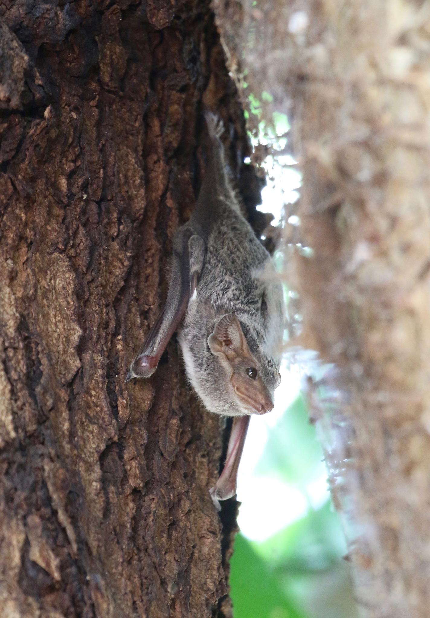
Cover caption A
Image:
and their conservation.
Mauritian
11, Mariette
tomb bat (Taphozous mauritianus). In an article on page
Pretorius asks why bat fossils in Africa are so rare, and how this rarity impacts our understanding of modern bats
CC-BY-NC) Shane Redelinghuys National Institute for Communicable Diseases, South Africa Commentary Preprints, press releases and fossils in space: What is happening in South African human evolution research? Robyn Pickering, Dipuo W. Kgotleng 17 Radio communications through rock strata – South African mining experience over 50 years Brian A. Austin 20 Navigating the JIBAR transition: Progress, impacts, readiness, and analytical insights Mesias Alfeus 27 Without access to social media platform data, we risk being left in the dark Douglas A. Parry 33 Research Article Why so few Ps become As: The character, choices and challenges of South Africa’s most talented young researchers Jonathan Jansen, Cyrill Walters, Alistair White, Graeme Mehl 36 Selection, sequencing and progression of content in biology in four diverse jurisdictions Edith R. Dempster 43 Climate finance across sub-Saharan Africa: Decision trees and network flows Queensley C. Chukwudum 53 AgERA5 representation of seasonal mean and extreme temperatures in the Northern Cape, South Africa Jacobus A. Kruger, Sarah J. Roffe, Adriaan J. van der Walt 65 Analysing patient factors and treatment impact on diabetic foot ulcers in South Africa Maxine J. Turner, Sandy van Vuuren, Stephanie Leigh-de Rapper 78 Sanguinarine highly sensitises breast cancer cells to doxorubicin-induced apoptosis Manisha du Plessis, Carla Fourie, Heloise le Roux, Anna-Mart Engelbrecht ............................... 87 Development of unsupported IrO2 nano-catalysts for polymer electrolyte membrane water electrolyser applications Simoné Karels, Cecil Felix, Sivakumar Pasupathi 99 Evaluation of pesticide residues and heavy metals in common food tubers from Nigeria Kingsley O. Omeje, Benjamin O. Ezema, Sabinus O.O. Eze 108 We the hunted Jesse M. Martin, A.B. Leece, Andy I.R. Herries, Stephanie E. Baker, David S. Strait 115
©skvorpahl on iNaturalist (


Working across disciplines: Robust debate in a context of trust
Search through the pages of the South African Journal of Science, and you will find hundreds of articles using the word ‘interdisciplinary’ and its variants, and the references to interdisciplinarity are almost invariably positive. Indeed, in the mission of the Journal (https://sajs.co.za/about) we describe the Journal as ‘multidisciplinary’ in its nature, and we have often in editorials and elsewhere referred to scientists from a range of disciplines working together.
Leavingasidethecomplex(and,paradoxically,oftenabstruse)arguments about the differences between interdisciplinarity, multidisciplinary, and transdisciplinarity, our Journal is part of a large consensus in which we need many ways of tackling difficult and complex problems, and none of us can provide the single ‘right’ answer to any of these. Especially in a fraught, divided and very unequal society, there is almost inevitably a social component to every technical problem, for example.
Our commitment to working and communicating across disciplines can be frustrating to potential authors and reviewers. We do not publish excellent work which is accessible only to a small disciplinary section of our readership. A number of emerging scholars have been, we fear, disheartened when their high-quality work is rejected, not because of concerns about the quality of the science, but because of the lack of accessibility to a non-specialist educated audience. Some authors have been trained to express their work using rather abstruse phraseology and syntax that is difficult to understand. Our Journal is certainly not the only one internationally committed to clear, plain, language usage (see https://sajs.co.za/inclusive-language-policy),butwithaninterdisciplinary journal, the bar is probably higher than with other journals, because words and usage conventions which are common currency in one discipline may not be familiar to readers in other disciplines.
Working across disciplines is also challenging for our editorial team. Each editor-in-chief comes from a particular disciplinary background, and it is not possible for this person, however competent, to assess fully the scientific quality of every submission. We are fortunate to have a team of very well-qualified associate editors and associate editor mentees, all of whom are subject specialists, and it is common at our Journal for the editor-in-chief to ask the appropriate associate editor for advice about whether to send a submission for review. Sometimes this process is even more complicated when we involve two or more associate editors in discussion before taking a decision about how best to handle a submission. This requires teamwork and coordination, and on reasonably rare occasions we have to ask for help from experts outside our small team if we do not have all the expertise. This takes effort –including anonymisation of submissions, confidentiality agreements, and so on, even before we decide on peer reviewers. It is simply not possible to have an editorial team which is expert in every possible sub-discipline which may be the home sub-discipline of a potential contributor.
At our Journal, we are fortunate to have good relationships within our team, so we are able to consult one another. This includes notionally less ‘senior’ colleagues, such as associate editors, informing notionally more ‘senior’ colleagues, such as the editor-in-chief, that they are wrong. In an ideal world, robust and open debate is at the heart of good science – we move forward as scientists and as a scientific community by changing
HOW TO CITE:
our minds, adjusting to new evidence and techniques. But there is an interpersonal element to this, and this is the element of trust. In order to differ openly with a colleague, one has to have the confidence that this expression of difference will not be seen as vexatious, undermining, rude, or inappropriate.
This need for trust in interdisciplinary relationships and research is not just a question for a journal like ours – it is essential for all research partnerships across disciplines. It is easy to speak about interdisciplinary respect and trust, but there can be challenges in attaining it. Many researchers have been trained to lionise their own disciplines and to denigrate others. For example, there are quantitative researchers who have been trained to consider all qualitative data as ‘mere anecdote’, just as there are qualitative researchers who have been trained to see their own work as ‘deep’ and ‘careful’, with the implication being that the work of quantitative researchers is of necessity superficial and conducted without due care. It is unfortunately the case that there are indeed many qualitative researchers whose work could fairly be characterised as merely anecdotal, just as there are many quantitative researchers who conduct superficial and slapdash work. There are bad researchers in all disciplines. But stereotyping researchers from other disciplines as the ‘other’ is not helpful. But there are other, perhaps less obvious, dangers. Just as it is not helpful a priori to decide that work from Discipline X is inferior or useless, it can be equally problematic for interdisciplinary research to take the opposite view – that work from Discipline X is inevitably good and helpful. Interdisciplinary respect is much more challenging than simply declaring that the work of colleagues in other disciplines is good, even when, and possibly especially when, one does not fully understand the methods used by those from other disciplines. There has to be space both for challenging interdisciplinary questions and for frank discussions about methods and conclusions. In the end, it may not be fully possible to understand what a colleague from another discipline has done, as it may take full academic training in that discipline to understand the colleague’s assumptions and methods. But asking questions across disciplines is important, and being prepared to try to answer questions across disciplines is equally important. It is not respectful simply to take for granted that another researcher must be right just because their work is not immediately understandable across disciplines. Disciplinary defensiveness may be more common in disciplines of ‘lower status’ than others, although I am unaware of good data to support this supposition, but disciplinary defensiveness (as opposed to standing up for and explaining the strengths of an approach one is taking) may close down debate and may well be bad for interdisciplinarity.
In an academic world in which competition across disciplines and amongst scientists is commonly encouraged, in a world in which many of us compete for the same resources, the temptation either unfairly to denigrate the other or to praise the other without robustly interrogating their work, are two sides of an unhelpful coin. Academic conflict, furthermore, can both flourish and be inappropriately avoided in a divided and high-conflict society. We believe that it is the collective responsibility of all researchers to keep real, robust, debate going. This takes trust both in others and in the academic system which sustains us all.
1 Volume 120| Number 3/4 March/April 2024 https://doi.org/10.17159/sajs.2024/18031 Leader
Swartz L. Working across disciplines: Robust debate in a context of trust. S Afr J Sci. 2024;120(3/4), Art. #18031. https://doi.org/10.17159/sajs.2024/18031
Author:
Quarraisha Abdool Karim1,2
AFFILIAtIoNS:
1Centre for the AIDS Programme of Research in South Africa (CAPRISA), Durban, South Africa
2Mailman School of Public Health, Columbia University, New York, New York, USA
CorrESPoNDENCE to:
Quarraisha Abdool Karim
EMAIL:
Quarraisha.abdoolkarim@caprisa.org
hoW to CItE:
Abdool Karim Q. Hoosen (Jerry)
M. Coovadia (1940–2023): Caring paediatrician, excellent scientist, courageous human rights activist and visionary leader. S Afr J Sci. 2024;120(3/4), Art. #17475. https:// doi.org/10.17159/sajs.2024/17475
ArtICLE INCLuDES:
☐ Peer review
☐ Supplementary material
PubLIShED:
27 March 2024
Obituary
Hoosen (Jerry) M. Coovadia (1940–2023): Caring
paediatrician, excellent scientist, courageous human rights activist and visionary leader
On 4 October 2023 the world mourned the loss of a caring paediatrician, an excellent scientist, a courageous human rights activist and a visionary leader. Professor Hoosen Mohamed Coovadia, fondly known as ‘Jerry’, was an exceptional and rare human being who blessed many lives – as a mentor, role model, colleague, and dear friend. He was an extraordinary human being who stood steadfast and unwavering for truth and justice, regardless of personal sacrifices and consequences. We have said goodbye to one of South Africa’s greatest scientists and staunchest proponents of democracy and equality. He stood well above others in his integrity and unwavering commitment to a just world.
South African President Cyril Ramaphosa said in a statement:
Our nation’s loss will be felt globally, but we can take pride at and comfort from the emergence of a giant of science and an icon of compassion and resilience from our country.
Like many whose lives Professor Coovadia touched, one was left deeply impressed by his incisive and profound contributions to both scientific and political discussions. He was an unparalleled intellect and leader who never compromised on anything less than world-class excellence. As an academic, he always had so much to share, teach and instil in eager, young minds and the number of outstanding medical students, paediatricians and scientists he nurtured and graduated are a testament to his life-changing mentorship and leadership. His passion for science and the way he effortlessly transformed complex medical challenges into a series of achievable research questions was truly inspiring. His inimitable curiosity and systematic approach did not compromise on the robust rigour that he applied equally in the way he cared for his young patients. As a mentor, he set a high bar, repeatedly pushing the boundaries of knowledge and expecting no less from his mentees. He was consistently magnanimous with his guidance and generous with the time he committed to nurturing, advising and supporting each and every one of his students. I was truly blessed and privileged to have him as my mentor for almost 35 years and I owe much of my success to his wise guidance and to being an inspiring role model on how to serve humanity with humility and equanimity. The respect and warmth he gave to his students resulted in lifelong friendships that extended to their entire families and often included multiple generations. His textbook Coovadia’s Paediatrics and Child Health, now in its 8th edition, is the go-to reference for thousands of medical students and paediatricians across Africa and in other low- and middle-income countries.
His passion for science was matched by his passion for freedom and justice for all. His prominent role in the struggle for a democratic South Africa and his principled stand against non-racialism were consistent with his character and with his always speaking to truth and doing what was morally the right thing to do.
Although he started his medical studies at the University of Natal in South Africa, he completed his medical degree in the 1960s at Grant Medical College in Bombay, where he met his lifelong partner and wife-to-be, Dr Zubie Hamed. Upon his return to South Africa following graduation, he worked at King Edward VIII Hospital and subsequently joined the Department of Paediatrics at the University of Natal Medical School, where he specialised in paediatrics and became a Fellow of the College of Paediatricians of the College of Medicine of South Africa in 1971. In 1974, he obtained his MSc in Immunology from the University of Birmingham in the UK.
It was his time at Grant College that was pivotal in terms of his political conscientisation. He was instrumental in forming a political body called the South African Students Association, which invited members of the African National Congress in exile, such as Dr Dadoo, to address them on freedom and the anti-apartheid movement. He was one of the key figures to rekindle the Natal Indian Congress in the 1970s and was subsequently elected its vice-president. In the 1980s, he was a key player in launching the United Democratic Front.
Politics and health were two sides of the same coin for him. He fought for equitable health care and was a founding member of the National Medical and Dental Association (NAMDA), which was set up by progressive doctors following the Medical Association of South Africa’s complacency regarding the doctors who were complicit in Steve Biko’s death.
He was formidable as an anti-apartheid activist – strategic and penetrating in his analysis of the tactics needed to advance the struggle for freedom. In the 1980s, he was part of a delegation to meet the African National Congress in Lusaka prior to the organisation being unbanned. He took part in the preliminary discussions and negotiations at the Congress for a Democratic South Africa (CODESA). As a result of his political activities, Professor Coovadia was targeted by the apartheid regime – his house was bombed during the political turbulence in the early 1990s, but he remained steadfast and undeterred from his commitment to a just and free South Africa.
Professor Coovadia’s research contributions on the effects of poverty and malnutrition on child survival and development included the definitive work on nephrosis in black South African children, malnutrition and immunity, and measles. His research focus pivoted to paediatric HIV/AIDS in the early 1990s as he started to witness the unfolding tragedy in his paediatric wards at King Edward VIII Hospital in Durban. His particular focus was the transmission of the virus from mother to child, a field in which he challenged conventional wisdom about breastfeeding and became nationally and internationally recognised for his groundbreaking research on saving babies’ lives by reducing HIV transmission from mother to child through exclusive breastfeeding.
2
Volume 120| Number 3/4 March/April 2024
https://doi.org/10.17159/sajs.2024/17475
© 2024. The Author(s). Published under a Creative Commons Attribution Licence.
He was appointed Chairperson of the inaugural Scientific Advisory Board to the Ministry of Health’s National AIDS Programme established post-1994 and he served as the first international co-chair of the US National Institutes of Health Global Paediatric Network for AIDS research. His international stature in HIV/AIDS led to him being appointed as Chairperson of the XIIIth International AIDS Conference in Durban in July 2000. This conference is widely credited for expediting access to AIDS treatment in poor countries. It brought him national and international accolades but also resulted in clashes with some prominent government figures at the time, especially President Mbeki and Minister TshabalalaMsimang. He undauntedly stood up to these AIDS denialists. Despite being vilified by some for his clashes with the President, Professor Coovadia persisted in speaking truth to power regardless, never faltering.
His leadership role in numerous national and global expert committees on health following his retirement as Chair of the Department of Paediatrics, including as President of the South African Medical Association, is a testament to his invaluable academic contributions. He was appointed the Victor Daitz Chair in HIV/AIDS Research, and Director of Biomedical Science at the Centre for HIV/AIDS Networking (HIVAN) at the Nelson R Mandela School of Medicine, University of Natal, and thereafter to the leadership of the Centre for the AIDS Programme of Research in South Africa (CAPRISA). In 2010, he was appointed to the government’s National Planning Commission to guide the development plan of South Africa. He spoke extensively on South Africa’s need for a National Health Service, with National Health Insurance as a stepping stone, being built on the foundations of primary health care. An unfinished dream he had was of restoring the abandoned Addington Children’s Hospital on the Durban beachfront to the KwaZulu-Natal Children’s Hospital of Excellence for the care of children with special health needs.
Professor Coovadia was the recipient of numerous distinguished and prestigious accolades and awards including the Star of South Africa and the Nelson Mandela Award for Health and Human Rights for his contributions to democracy and health. He received honorary doctorates from the Universities of Durban-Westville, Witwatersrand and Cape Town. He is one of a handful of South Africans to be elected as a Foreign Member of the US National Academy of Medicine. He received the
Science-for-Society Gold Medal award of the Academy of Science of South Africa; the American Association for the Advancement of Science Scientific Freedom and Responsibility Award; a Lifetime Achievement Award during the HIV Congress in India; a Silver Medal for Excellence in Research (Medical Research Council); the SAMRC Presidential Award; the International Association of Physicians in AIDS and Care Award; and the Heroes in Medicine Award in Toronto, Canada.
Professor Coovadia was a patriot; he was deeply committed to a better and more just South Africa. He was a fierce critic of maladministration and corruption in government and was vocal about how he felt that the struggle for a free and just country was being jeopardised by greed and incompetence. A few years ago, he developed weakness in both limbs, which progressively deteriorated until he became wheelchair-bound. Notwithstanding his health challenges, he remained in good spirits and those who visited him benefitted from engaging in conversations on life, literature, global politics and new developments in science.
In an interview with the Academy of Science of South Africa in 2017, when asked what people don’t know about him, Coovadia responded: “Despite some corroding bourgeois proclivities, I remain at heart and in mind, an adherent of equity and fairness in all things meaningful — justice for the poor and the elimination of poverty.”
We pay tribute to his wife Dr Zubie Hamed, son Professor Imraan Coovadia and daughter Dr Anushka Coovadia, their children and his extended family for their support during his many years spent fighting for social justice and establishing a strong science base in South Africa.
We have lost a visionary who remained forever hopeful that South Africa would be a great country, one who cared for the poor and most vulnerable, notably its children. We have lost an icon in the world of medical science, unwavering in his commitment to saving lives through his research. We have lost a giant who towered above others in his steadfast and unwavering integrity and compassion. His demise has left us with a deep sense of loss, but his legacy lives on in all the lives he touched.
Hamba kahle Professor Jerry Coovadia.
Volume 120| Number 3/4 March/April 2024 3 https://doi.org/10.17159/sajs.2024/17475 Obituary Jerry Coovadia (1940–2023) Page 2 of 2
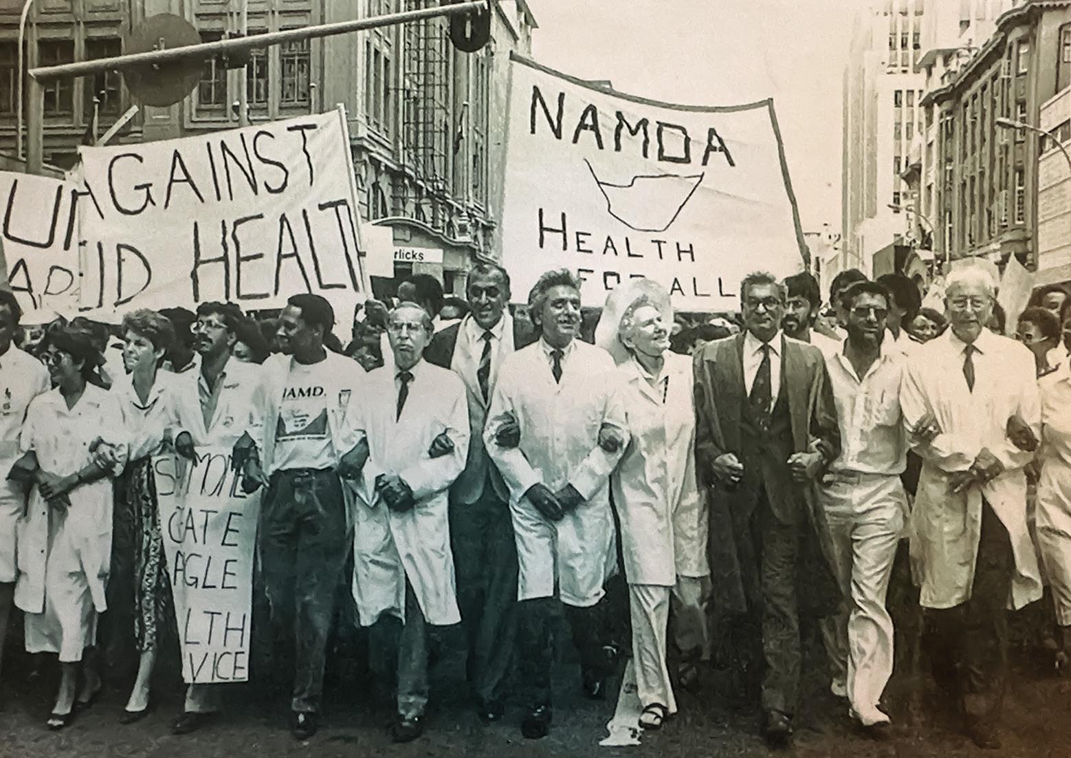
Professor Jerry Coovadia fought for equitable health care and was a founding member of the National Medical and Dental Association (NAMDA).
Source: CAPRISA archives
BOOK TITLE: Statues and storms: Leading through change

AuThOr:
Max Price
ISBN:
9780624087762 (paperback, 320 pp)
PuBLIShEr: Tafelberg Publishers, Cape Town; ZAR350
PuBLIShEd: 2023
rEVIEWEr: Michael I. Cherry1
AFFILIATION:
1Department of Botany and Zoology, Stellenbosch University, Stellenbosch, South Africa
EMAIL:
mic@sun.ac.za
hOW TO CITE: Cherry MI. The storms facing higher education have not abated. S Afr J Sci. 2024;120(3/4), Art. #17274. https://doi.org/10.17159/ sajs.2024/17274
ArTICLE INCLudES:
☐ Peer review
☐ Supplementary material
PuBLIShEd: 27 March 2024
The storms facing higher education have not abated
Spare a thought for Max Price, who had a successful first term as Vice-Chancellor of the University of Cape Town (UCT) from 2008 to 2013. He knows his onions, visited departments regularly and was popular with academic staff: his contract was renewed for a second term. Until Chumani Maxwele threw poo on Rhodes’ statue soon after the start of the second term in 2015, Price could not have foreseen that the time was out of joint.
Statues and Storms is the account of his torrid time over the next three years, during which Price was assaulted, had his laptop snatched and his office fire-bombed. The book is well written and well edited – editor Russell Martin excised a third of the original text, although Price “still thinks every word of it should have been retained.”
There is little to fault Price’s handling of events during the first year of the crisis in 2015. Although he had ignored Rhodes’ gaze for nearly eight years, he was not the first vice-chancellor to do so. But since its removal in April 2015 the statue has not been missed, and perhaps one day it will be displayed elsewhere, appropriately contextualised. A second demand, the in-sourcing of workers, redressed (at least to some extent) the shameful manner by which they had been outsourced in the late 1990s.
The third – and least tractable – demand was a national one for free higher education. Here government, having faced off national demonstrations both outside parliament and at the Union buildings, had set up yet another commission, this time under retired Judge Heher, to investigate it.
Then, at the beginning of 2016, things spun out of control. Price found himself unable to set clear boundaries with a tiny group of students that threatened to disrupt campus life in a violent manner (it was unclear how much support this group commanded as it did not comprise elected representatives, but very clear that it espoused a particularly toxic form of racial identity politics). In not doing so, as Nicoli Nattrass perceptively remarks1, Price “was legitimising a politics of racialised offence”. Combined with his conspicuous lack of any successional planning, this has been his legacy to UCT.
Price’s book is remarkable for its lack of humility. With the certainty of a colonial administrator, he justifies his every turn, claiming that his leadership blazed a trail for institutions both here and abroad. What is unclear is how his strategy is reconcilable with his articulated view (p. 280): “In a society where the laws are unjust, civil disobedience, i.e. unlawful behaviour, may be justified. Today, we live in a constitutional democracy in which the majority can exercise their voices without resorting to civil disobedience.”
For a seasoned campaigner he also reveals a curious naïveté, for example in appearing disappointed when the Heher Commission did not report in time, and more so when government discarded its recommendations altogether.
Really? Wishing away pragmatic solutions had become a favourite pastime of Minister of Higher Education Blade Nzimande (the real villain of the piece), who had ignored a report on the feasibility of free higher education chaired by former Nelson Mandela University Vice-Chancellor Derrick Swartz.2 And Nzimande had also shelved two related reports: on the future of university funding (chaired by none other than Cyril Ramaphosa); and a review of the National Student Financial Aid Scheme (NSFAS), chaired by Marcus Balintulo, former Vice-Chancellor of Walter Sisulu University.
Price does not provide much scholarly examination of the deeper issues underlying the protests – for this readers can turn to David Benatar’s The Fall of UCT, although Ronelle Carolissen has noted that it lacks context on the corporatisation of universities this century.3
It seems unclear to Price why he appeared as the embodiment of this corporatisation, but it is in this context that his account is instructive. This century South Africa has experienced a large expansion in student numbers, together with below-inflation subsidy increases, leading inevitably to fee increases well above inflation.
David Attwell, also reviewing Benatar’s book, makes another crucial point about context4: “For local students, the venality of state capture and corruption, the very real prospect of state failure, has opened up a profound moral abyss. We have a democratically elected government that is failing.”
Both criticisms apply equally well to Price’s book. In this context, a general decline in institutional loyalty is unsurprising. In particular, many black students attending historically advantaged institutions experience a feeling of alienation to the point that little respect for institutional culture or infrastructure exists. The challenge to our universities is to re-build that loyalty.
Beyond Price’s legacy to UCT, that of #FeesMustFall has been of profound national significance. In December 2017, campaigning to be re-elected as ANC President, Zuma announced that government had rejected the Heher recommendations (an income-contingent loan scheme, loans being recovered by the South African Revenue Service once the graduate’s income reaches a certain threshold). Instead it would provide fees and maintenance grants (as opposed to loans) to university students with a household income below ZAR350 000 per annum –almost doubling the previous threshold of ZAR180 000.
Ramaphosa chose to implement this, and the consequences have not been trivial. The NSFAS budget has risen more than threefold (from ZAR15 billion to ZAR50 billion) between 2017 and 2023.5 NSFAS now receives 53% of the higher education budget, with the country’s 26 public universities receiving the
4 https://doi.org/10.17159/sajs.2024/17274 Volume 120| Number 3/4 March/April 2024 © 2024. The Author(s). Published under a Creative Commons Attribution Licence. Book Review
remainder in subsidies. The original problem – above-inflation fee increases – has not been resolved.
Free university education might be affordable if student numbers were capped – no bad thing if this were to be matched by a significant expansion in the vocational training component of our higher education system. The principle that the state should set the number of subsidised university places nationally in each discipline was adopted in the 1997 White Paper on Higher Education.6 Twenty-six years on we are still awaiting the implementation of this policy. What remains of the NSFAS, once corruption has claimed its share, has instead become a social grant for young people, the majority of whom sadly never graduate.2
references
1. Nattrass NJ. The man who saw the abyss...only to fall into the gutter of race. Business Day. 2023 September 26. Available from: https://www.businesslive. co.za/bd/life/books/2023-09-26-big-read-the-man-who-saw-the-abyss-only-to-fall-into-the-gutter-of-race/
The storms facing higher education have not abated Page 2 of 2
2. Cherry MI. Four years later and Nzimande has still not acted on higher education reports. Business Day. 2016 October 24. Available from: https:// www.businesslive.co.za/bd/opinion/2016-10-24-four-years-later-andnzimande-has-still-not-acted-on-higher-education-reports/
3. Carolissen R. Ivory towers as contested spaces: A review of The Fall of the University of Cape Town. S Afr J Sci. 2022;118(9/10), Art. #13916. https:// doi.org/10.17159/sajs.2022/13916
4. Attwell D. On The Fall of the University of Cape Town by David Benatar: A discussion.LitNet.2022January11.Availablefrom:https://www.litnet.co.za/ on-the-fall-of-the-university-of-cape-town-by-david-benatar-a-discussion/
5. Du Plesssis S. NSFAS has failed our students, universities and country. Business Day. 2023 October 25. Available from: https://www.businesslive. co.za/bd/opinion/2023-10-25-stan-du-plessis-nsfas-has-failed-ourstudents-universities-and-country/#google_vignette
6. Cherry MI. South Africa reforms university funding. Nature. 1997;387:327. https://doi.org/10.1038/387327a0
Volume 120| Number 3/4 March/April 2024 5 https://doi.org/10.17159/sajs.2024/17274 Book Review
BOOK TITLE: Recasting workers’ power: Work and inequality in the shadow of the Digital Age

AuThORs: Edward Webster, Lynford Dor, Kally Forrest, Fikile Masikane, Carmen Ludwig
IsBN:
9781776148820 (paperback, 208 pp)
PuBLIshER: Wits University Press, Johannesburg; ZAR300
PuBLIshEd: 2023
REVIEWER: Mondli Hlatshwayo1
AFFILIATION:
1Centre for Education Rights and Transformation, University of Johannesburg, Johannesburg, South Africa
EMAIL: mshlatshwayo@uj.ac.za
hOW TO CITE: Hlatshwayo M. From casting to recasting: Reviewing the Recasting of Workers’ Power. S Afr J Sci. 2024;120(3/4), Art. #17840. https:// doi.org/10.17159/sajs.2024/17840
ARTICLE INCLudEs:
☐ Peer review
☐ Supplementary material
PuBLIshEd: 27 March 2024
From casting to recasting: Reviewing the Recasting of Workers’ Power
In 1985, Eddie Webster’s book entitled Cast in a Racial Mould: Labour Process and Trade Unionism in the Foundries1 was published by Ravan Press. Among many other things, the book discusses how iron and steel moulds of the East Rand near Johannesburg cast or divided workers according to their skin colour, where white workers and their unions had to struggle over many years to defend and advance their privileges at the workplace. On the other hand, the book, which became one of the critical knowledge foundations of Labour Studies in South Africa and the world over, demonstrates how black workers in South Africa’s metal sector were able to cast their net wide by building a trade union called the Metal and Allied Workers Union (MAWU), which became the shield and spear of black metal workers.
Webster and his team’s most recent book, Recasting Workers’ Power: Work and Inequality in the Shadow of the Digital Age, reveals how work and the labour processes have changed since the 1990s (p. ix–xiv). The recent book analyses and discusses an entirely different world of work from that in the 1980s. The resistance workers ‘cast in a racial mould’ were the black industrial proletariat, who were often regarded as blue-collar workers who were the core of the workforce that confronted what von Holdt2 characterised as the “apartheid workplace regime”. The militant layer’s political and organisational leverage waned as the manufacturing sector declined in the 1990s.
In some ways, the “recasting of workers’ power” is about the second phase of workers’ power since the 1970s and the 1980s. A new social force is being born to replace the old one. The changing nature of work, the deepening oppression of workers, and the weaknesses of trade unions are recasting or reshaping an extremely precarious workforce working in the informal economy, digital spaces, and factories. Despite being weakened by capital, these workers are finding ways to recast their power to resist extreme forms of subjugation in labour.
Like in Cast in a Racial Mould, Webster and his team adopt dualism to unpack workers’ oppression and resistance in South Africa, Uganda, Kenya, and other countries. The observations, in-depth interviews, and documentary analysis are deployed to reveal the duality of oppression and resistance in the labour processes. In other words, this ethnographic approach enabled Webster and his team to show new organisational forms emerging in the formal and informal economies of the Global South, disputing the perspective that neoliberal globalisation has ultimately defeated the workers of the Global South. Of course, Webster and his team understand that the workers of the Global South are engaged in what I describe as an asymmetrical warfare persecuted by the states, businesses, and the powerful forces of the Global North.
However, workers discussed in the recent book have various forms of power in this asymmetrical warfare. To this end, this new book examines organising strategies through the prisms of three other forms of power: coalitions (the power of society), associational power (the power of collective organisation), and institutional power (the laws that uphold labour rights).
The book also makes the case that labour is still relevant by deploying various sources and forms of worker power. Webster and his colleagues assert that precarious workers, including digital workers, are redefining their resistance to the growth of precarious forms of labour. The book acknowledges that workers and trade unions have been undermined by capitalists. Trade union density, or the rate at which employees join unions, has decreased both globally and in South Africa, which is one indication of this reality.
Webster rejects the “end of labor thesis” (p. ix) and demonstrates that even the most alienated platform workers possess the capacity for individual and collective resistance against complete subjugation by capitalist and platform systems. Webster and Dor’s work (Chapter 4) transcends mere analysis of the issues of digital oppression and offers a sense of hope for labour, particularly within the context of the Global South. Despite all the challenges confronting platform workers in South Africa and the Global South, this is true. Masikane also shows that, notwithstanding the formidable algorithms in place, the collective strength of smartphone-based platforms thwarted the operations of Uber Eats in December 2020 (p. 101–124). This resistance compelled platform employees to impose a fixed fee of EUR0.50 for each delivered meal.
As a scholar and activist who witnessed the rise and decline of manufacturing workers and their trade unions, Webster has not given up hope on labour, despite its changes in shape and form. As he was with the workers who led the Durban strikes of 1973, he is now with the platform economy workers, informal workers, and precarious workers searching for an organisational response in this asymmetrical war against this new form of vampire capitalism.
References
1. Webster E. Cast in a racial mould: Labour process and trade unionism in the foundries. Johannesburg: Ravan Press; 1985.
2. Von Holdt K. Social movement unionism: The case of South Africa. Work Employ Soc. 2002;16(2):283–304. https://doi.org /10.1177/095001702400426848
6 https://doi.org/10.17159/sajs.2024/17840 Volume 120| Number 3/4 March/April 2024 © 2024. The Author(s). Published under a Creative Commons Attribution Licence. Book Review
BOOK TITLE: Violent ecotropes: Petroculture in the Niger Delta
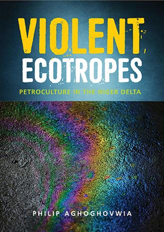
AuThOr:
Philip Aghoghovwia
ISBN: 9780796926180 (paperback, 260 pp)
PuBLIShEr: HSRC Press, Cape Town, ZAR267
PuBLIShEd: 2022
rEVIEWEr: Christopher M. Mabeza1
AFFILIATION:
1Women’s University in Africa, Harare, Zimbabwe
EMAIL:
cmmabezah@gmail.com
hOW TO CITE:
Mabeza CM. And the band played on: Conflict-preneurship and the long history of violence in the Niger Delta. S Afr J Sci. 2024;120(3/4), Art. #17568. https://doi.org/10.17159/sa js.2024/17568
ArTICLE INCLudES:
☐ Peer review
☐ Supplementary material
PuBLIShEd:
27 March 2024
©
Book Review
And the band played on: Conflict-preneurship and the long history of violence in the Niger Delta
As I read Philip Aghoghovwia’s Violent Ecotropes: Petroculture in the Niger Delta, I could not help but appreciate the echoes of Rob Nixon's1 Slow Violence and the Environmentalism of the Poor. The slow violence in the Niger Delta is an ugly symptom of a runaway extractive economy. The adage, ‘the more deadly virus is not HIV/Aids, it is greed’, comes to mind. In this publication, the greed is not only confined to an enduring capitalist system but also local elites, something akin to what Umair Haque terms “a class of billionaires so amoral they’d make Caligula blush”2. It is because of this class of ‘conflict-preneurs’, to borrow a term from Akufo-Addo3, that the violence has continued unabated in the Niger Delta.
Luis Fernández Carril, writing about the staying power of capitalism in his essay, The Ontological Crisis of the Anthropocene, could not have agreed more:
Life, capitalism, modern institutions, and political and economic systems seem inevitable, perennial, and immortal. As captured by the now famous adage: It is easier to imagine the end of time than to imagine the end of capitalism.4
Violent Ecotropes: Petroculture in the Niger Delta offers a well-articulated and timely analysis of a major theme in contemporary development studies. The book engages local epistemologies and ontologies on the violence in the Niger Delta. Aghoghovwia’s masterful use of literary works published between 1998 and 2015 points to the reality that the violent ecotropes are not a black swan event but a manifestation of local people’s struggles from the colonial era. The author is to be commended for articulating perspectives from those who live on the margins of history. Violence is a recurring theme in the poetry collections of the Delta, an issue that is troubling to the author.
Chapter 1 uses plays to “depict a tragic reality that attends everyday human existence in the Delta environment.” The chapter grapples with the flaws of modernity as encapsulated by the Delta. The author attributes this to power struggles and coins the term petromodernity. Petromordenity is about making huge profits at a huge cost to the communities and the environment.
In the second chapter, the author uses fire as a metaphor. The chapter focuses on Ogaga Ifowodo’s The Oil Lamp (Africa World Press, 2006). The Oil Lamp shows how fire is destructive to the environment. Fire is used as a metaphor for the destructive nature of neoliberalism. Neoliberalism with its attendant apocalyptic horsemen (disease, poverty, violence) wreaks havoc on the communities. Ifowodo and a host of writers “put under the spotlight the overwhelming social and ecological deprivations suffered by the citizenry, the denial of basic rights, and the fate of the postcolonial nation under corrupt military regimes.”
Chapter 3 discusses the latent violence in the Delta. Ibiwari Ikiriko’s Oily Tears of the Delta (Kraftgriots, Ibadan, 2000) depicts how the infrastructure of oil extraction becomes an arena of contested power. Oily Tears is a call to arms. The literary works in this chapter are critical of what the author terms “oily” intrusions into the Delta. The “oily” intrusions have caused a lot of suffering as seen by the displacements in the Delta.
Chapter 4 analyses the Nollywood film The Liquid Black Gold (Executive Image African Movies, 2008). The Liquid Black Gold grapples with the violence associated with oil extraction in the Delta. According to Aghoghovwia, The Liquid Black Gold discusses the generational rivalry between the young and the old, a product of a gerontocracy culture. This has resulted in tensions in the communities. The chapter also draws on the works of Frantz Fanon (The Wretched of the Earth, Grove Press, 1961) and Rob Nixon (Slow Violence and the Environmentalism of the Poor). Fanon’s work is premised on resisting imperialism. Nixon argues about the impact of what he terms “slow violence” on the locals and the environment.
The author shows the complexity of the Niger Delta conflict. On one hand, there is the brutality of international capital, and on the other, is the evil nature of the disaster of capitalism as encapsulated by local conflict entrepreneurship. The book reflects the Hobbesian nature of life which is nasty, brutish and short. The people in the Niger Delta have suffered for so long. There seems to be no light at the end of the tunnel. One is inclined to argue that solutions that have been and are being proffered to solve the conflict in the Delta amount to Orwellian dishonesty and Potemkin facades meant to hoodwink the local communities.
In line with the above observations, the title of Mary Trump’s book Too Much and Never Enough5 resonates with the insatiable greed of the Delta Region’s conflict-preneurs, who have realised that the spoils of conflict far outweigh initiatives for peace. They have benefitted handsomely from the conflict, and so they have dug in. A term in the field of disaster management used about conflict-preneurship is disaster capitalism. Disaster capitalism is the use of catastrophe in conflict and post-conflict situations to promote and empower a range of private, neoliberal capitalist interests. What is being witnessed in the Niger Delta is disaster capitalism, therefore the use of the term could have enriched the book.
Addressing environmental turmoil is fundamentally about advancing social justice. Questions of justice are critical to Violent Ecotropes. The author could have engaged more with the different dimensions of justice. These dimensions range from who gets what (distributional justice) and whose knowledge (epistemic justice), to who gets to decide (procedural justice) and ultimately who gets left behind (recognition justice).6
Also, Yuval Noah Harari’s overhasty jump theory7 could be useful in understanding the Niger Delta’s long history of violence. According to Harari, humans rose to the top of the food chain in a relatively short time. In a bid to solidify their position at the top, humans have become brutal. Humans will go out of their way to eliminate other
https://doi.org/10.17159/sajs.2024/17568
7
Volume 120| Number 3/4 March/April 2024
2024. The Author(s). Published under a Creative Commons Attribution Licence.
species (including their own) to remain at the top of the food chain. Thus, humanity’s overhasty jump is one of the major reasons for violence, and, I strongly believe, what hinders successful outcomes in a multi-species approach to environmental management. As already alluded to, humans will protect their place at the top of the food chain at any cost. Perhaps it is time to address humanity’s insecurity at the top of the food chain. Part of the solution is the realisation that a multi-species approach means a win–win for all species.
Violent Ecotropes is well articulated, intellectually stimulating and provides new knowledge about the conflict in the Niger Delta. The chapters are concise and make interesting reading. I therefore very highly recommend the book.
references
1. Nixon R. Slow violence and the environmentalism of the poor. Cambridge, MA: HarvardUniversityPress;2011.https://doi.org/10.4159/harvard.9780674061194
And the band played on Page 2 of 2
2. Haque U. The pattern of the 21st century is predatory collapse: The hidden thread running through a troubled age. Eudaimonia and Co. 2019 June 02. Available from: https://eand.co/the-pattern-of-the-21st-century-is-predatory-collapse-b06f93679cd
3. Mubarik A. Ward-off 'conflict-preneurs': Akufo-Addo urges Dagbon. Pulse. 2017 January 27. Available from: https://www.pulse.com.gh/news/local/war d-off-conflict-preneurs-akufo-addo-urges-dagbon/f1mtktm
4. Fernández Carril LC. The ontological crisis of the Anthropocene [webpage on the Internet]. No date [cited 2023 Dec 06]. Available from: https://www.weat hermatters.net/ontological-crisis-of-the-anthropocene
5. Huff A, Naess LO. Reframing climate and environmental justice. IDS Bulletin. 2022;53(4). https://doi.org/10.19088/1968-2022.133
6. Trump M. Too much and never enough: How my family created the world's most dangerous man. New York: Simon & Schuster; 2020.
7. Harari YN. Sapiens: A brief history of humankind. London: Penguin Random House; 2015.
Volume 120| Number 3/4 March/April 2024 8
Book Review
https://doi.org/10.17159/sajs.2024/17568
BOOK TITLE: Human trafficking in South Africa

AuThOr: Philip Frankel
ISBN: 9781928246589 (soft cover, 207 pp)
PuBLIShEr: BestRed, Cape Town; ZAR340
PuBLIShEd: 2023
rEVIEWEr: Monique Emser1
AFFILIATION:
1International and Public Affairs Cluster, School of Social Sciences, University of KwaZulu-Natal, Durban, South Africa
EMAIL: EmserM@ukzn.ac.za
hOW TO CITE: Emser M. Human trafficking: Misery and myopia in South Africa. S Afr J Sci. 2024;120(3/4), Art. #17393. https://doi.org/10.17159/ sajs.2024/17393
ArTICLE INCLudES:
☐ Peer review
☐ Supplementary material
PuBLIShEd:
27 March 2024
© 2024.
Book Review
Human trafficking: Misery and myopia in South Africa
Frankel’ssecondcomprehensivebooksurveyingthelandscapeofhumantraffickingandcounter-traffickinggovernance in South Africa, written during the COVID pandemic, offers a considered and nuanced account of this heinous and pervasive phenomenon. Frankel’s description of the diverse manifestations of the crime remains dispassionate and analytical throughout. Drawing from local research, international reports, indices, and measured media reports from 2016 onwards, as well as interviews conducted with key stakeholders, academic experts, victims, perpetrators, and civil society, Frankel weaves together a cogent narrative that is accessible to the wider public.
What sets Frankel’s work apart is twofold: (1) the inclusion of ‘outlier’ aspects of trafficking1 ignored by the vast majority of South African trafficking research; and (2) an interdisciplinary approach to understanding the phenomenon.
The book is divided into seven chapters. Frankel provides a foundation for understanding trafficking in persons from an international perspective in Chapter 1, as well as key concepts such as the nature of social vulnerability, the complexities of the trafficking process, and victim and perpetrator profiles. The controversial nature of trafficking and questions of prevalence are also addressed here. In the next three chapters, Frankel paints with broad brushstrokes how sex trafficking, child trafficking and labour trafficking manifest in the South African context. Frankel successfully offers a critical gaze on the state of human trafficking research, and the disproportionate focus by some researchers and policymakers on sex trafficking (historically to the disadvantage of other forms of trafficking). He further highlights the stark realities of child trafficking – and the often multiple, and concurrent, forms of exploitation children are forced to endure. Children are particularly vulnerable to being exploited for sex, labour, forced marriage, illegal adoption, and their organs. Child labour, also discussed in the chapter on the regional framework, is a particularly significant issue in both South Africa and the surrounding region. Labour trafficking, which is preeminent in Africa, and disproportionately affects male victims, who are predominantly exploited in agriculture, mining, and commercial fishing, does not receive as much attention in the South African context.
He illustrates the need to challenge stereotypical understandings of victims and perpetrators. Various criminal syndicates in the more organised forms of trafficking are also unpacked throughout these three chapters. What becomes apparent is that although human trafficking is understood as a clandestine crime, it is more often than not a crime hidden in plain sight. This is reflected in some offender profiles that mirror Hannah Arendt’s contention about the “banality of evil”1 and is particularly true in cases of ‘incidental trafficking’. A reoccurring theme throughout the book is the role that corruption and complicity of various state institutions play in the perpetuation of trafficking within South Africa – even more dangerous when apathy and self-interest are intermixed in a countertrafficking environment plagued by incapacitation of key stakeholders.
Having provided a conceptual understanding of the often-intersecting broad categories of trafficking, and the operational challenges that exist in successfully addressing them, Frankel turns his focus to counter-trafficking in South Africa, and the regional framework in Chapters 5 and 6. These two chapters provide a unique analysis that has not been well addressed in previous research. Frankel offers a comprehensive and analytical critique of counter-trafficking, and the legislative and policy framework within which it occurs, and its coordination structures. Frankel claims that “deficiencies in the PACOTIP create dysfunctionality in its key implementation vehicle...the policy framework is at this point in its existence a very weak tool for catching traffickers” (p. 109).
One of the most damning findings in the book is the penetration of the South African political economy by transnational criminal networks coupled with a relative absence of political will and capacity. This in turn plays out in the apparent reluctance of the criminal justice system to punish perpetrators commensurate with their crimes, and poverty of resources allocated to rehabilitation and reintegration systems for victims (p. 116). Issues that are similarly mirrored across the region.2 Chapter 6 then turns to the regional framework and the transnational nature of trafficking. As Frankel succinctly notes, “at a time of globalisation we cannot comprehensively understand trafficking within the Republic without reference to what takes place immediately outside its territory” (p. 124). The regional perspective is often lacking in South African trafficking research and/or strategic initiatives. Frankel discusses the regional threat matrix as witnessed in the six countries comprising the southern African region, and more generally in the Southern African Development Community (SADC). However, he does not survey the East African migration-trafficking nexus originating in Ethiopia and traversing through Kenya, Tanzania, Malawi and Mozambique. This is a minor critique – as the logic for his exploration of trafficking in the region is limited to southern Africa.
One of the book’s strengths is its commitment to not only highlight the problems but also to propose tangible solutions. Frankel’s ten-point counter-trafficking strategy is rooted in a deep understanding of the South African context, acknowledging the need for comprehensive and collaborative efforts. He advocates for capacity building and strengthening law enforcement, confronting corruption, improving victim support systems, mobilising civil society and a proactive approach to dismantling trafficking networks. Frankel delivers a clarion call to policymakers, civil society, and citizens alike to contribute meaningfully to the fight against human trafficking in South Africa.
references
1. Arendt H. Eichmann in Jerusalem: A report on the banality of evil. London: Penguin Classics; 2022.
2. Ras I, Els W. Southern Africa’s security hinges on actioning its organised crime strategy. ISS Today. 23 October 2023. Available from: https://issafrica.org/iss-today/southern-africas-security-hinges-on-actioning-its-organised-crime-strategy
https://doi.org/10.17159/sajs.2024/17393
9
Volume 120| Number 3/4 March/April 2024
The Author(s). Published under a Creative Commons Attribution Licence.
BOOK TITLE: Wildlife documentaries in southern Africa: From East to South
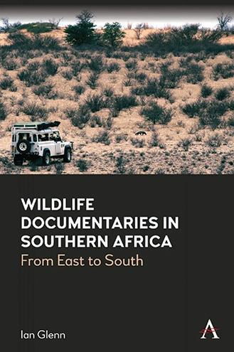
AuThOr: Ian Glenn
ISBN:
9781839981500 (hardcover, 286 pp)
PuBLIShEr: Anthem Press, New York, USA; USD125
PuBLIShEd: 2022
rEVIEWEr: Jacob S.T. Dlamini1
AFFILIATION:
1History Department, Princeton University, Princeton, New Jersey, USA
EMAIL: jdlamini@princeton.edu
hOW TO CITE: Dlamini JST. Ian Glenn’s ‘Wildlife Documentaries in Southern Africa: From East to South’. S Afr J Sci. 2024;120(3/4), Art. #17299. https:// doi.org/10.17159/sajs.2024/17299
ArTICLE INCLudES:
☐ Peer review
☐ Supplementary material
PuBLIShEd: 27 March 2024
Ian Glenn’s ‘Wildlife Documentaries in Southern Africa: From East to South’
When Theodore Roosevelt, the former US President, led a scientific expedition to Africa in March 1909, he chose east Africa as his destination. The safari, sponsored by the Smithsonian Institution, set out to collect big game, birds, mammals, reptiles and plants for the US National Museum in Washington DC. In the end, Roosevelt and his son Kermit, a first-year student at Harvard University who accompanied his father on the trip, killed and collected 512 animals. As Ian Glenn explains in his marvellous new book, it is not surprising that Roosevelt and his son chose east Africa for their expedition. Starting in the early 1800s, east Africa – to which the world owes the word safari (Swahili for journey) – was the world centre for so-called ‘big game hunting’. Any big game hunter worth their salt plied their trade in the region. In fact, Frederick Courteney Selous and Edward North Buxton, the world’s leading big game hunters of their day, helped arrange Roosevelt’s 1909 trip. Between the mid-1800s and the mid1900s, east Africa was the place to be for American and European hunters. It was also the destination of choice for monied tourists who wanted something other than old European cities for their vacations. It was not surprising, therefore, that when wildlife documentary emerged as a genre of filmmaking in the mid-20th century, east Africa occupied pride of place in that emergence. However, starting in the 1970s, east Africa began gradually to lose its place to southern Africa as both a premier tourist destination and the home of wildlife documentary filmmaking in Africa. Glenn’s book offers a compelling explanation of this change.
As Glenn explains, “The big idea of this book is that, starting in the early 1970s, wildlife films made in southern Africa, mostly but not exclusively by southern Africans, started winning major international awards and mark a crucial move away from east Africa as the centre of African wildlife film. More than that, they start influencing modern trends in the genre and provide some of its most important achievements” (p. 2). At the centre of Glenn’s wonderful book are many of these pioneering filmmakers, including Beverly and Dereck Joubert, who have won eight Emmys, as well as Carol Hughes and her late husband David who won six Emmys and a Golden Panda, the premier British prize for the best wildlife film of the year. The Hugheses won the very first Golden Panda award in 1982 for their 1979 film Etosha: Place of Dry Water (p. 1). This makes the Jouberts and the Hugheses South Africa’s most successful filmmakers, as measured by international accolades. Given the ubiquity of wildlife films, filmmakers such as the Jouberts and the Hugheses are also likely to be among the most watched in the world. Through a series of interviews with many of the leading wildlife filmmakers, Glenn takes the reader mercifully away from David Attenborough. In fact, Glenn cuts Attenborough down to size by showing how Attenborough himself drew direct and indirect inspiration from some of the filmmakers that Glenn writes about. Glenn does this through a masterful analysis of which filmmaker worked with whom, how one influenced another, and how they all created an extended network through which flowed ideas, influences and personalities. For example, while Attenborough was listed as the presenter of the 1987 BBC documentary Meerkats United, once voted by BBC viewers as the best wildlife documentary of all time, Attenborough’s role was basically limited to that of a voice-over artist. The South African Richard Goss made that film (p. 7–8).
As Glenn points out, “There is a massive disparity between popular interest in wildlife documentary and academic attention to the genre, particularly in southern Africa.” (p. 6) This means, among other things, that we have no reliable data on how many people actually watch these documentaries. We know they are popular the world over; we just can’t quantify that popularity. But we know from the awards won and the outsize influence that wildlife filmmakers from southern Africa have on the genre, that the region dominates the business. Part of the explanation for this dominance, Glenn argues, is that filmmakers from southern Africa have made the greatest use of new technologies (p. 8). They were also among the first to draw ethical implications from their work on wildlife. For example, Michael Rosenberg, a South African who spent most of his working life in London and won more Golden Pandas than any other wildlife filmmaker, produced Fragile Earth, one of the first series of documentaries to educate the public about environmental degradation and the importance of conservation; the Jouberts produced work that compared the emotional capacities of humans with those of elephants.
In his explanation of the shift in wildlife documentary filmmaking from east to southern Africa, Glenn argues that changes in wildlife policies in east Africa drove the shift. When, for example, Kenya banned hunting in 1977, hunters and filmmakers moved down south. This did not mean that the change in location was seamless. The Kruger National Park, for all its status as Africa’s most iconic reserve, had none of the vistas offered by the Serengeti. But, as Glenn reminds us, southern Africa had places such as the Kalahari and the Namib, which could more than compensate for what the Kruger lacked. The change in location ushered in new directions in wildlife documentary filmmaking, thanks to discoveries of phenomena not found elsewhere. Among these novel finds was the Jouberts’ discovery of a bitter rivalry in Botswana between large lion prides and hyaena clans. This led to Eternal Enemies, the 1992 award-winning film narrated by Jeremy Irons. One of my favourite stories in a book brimming with rich tales concerns the advent of open vehicles for game viewing. According to Glenn’s informants, Mala Mala and Londolozi, two private lodges in southern Africa, pioneered this. Then African trackers took it a step further by inventing and designing the tracker seat that is now standard in all safari vehicles. Robert Maluka, a technician in the Londolozi workshop, made the very first of these seats (p. 47).
In Wildlife Documentaries in Southern Africa, Glenn has given us a fun read and much-needed inspiration for future research. The public and scholars from across a range of disciplines are going to find in this book wonderful stories and excellent ideas.
© 2024. The Author(s). Published under a Creative Commons Attribution Licence.
Book Review
https://doi.org/10.17159/sajs.2024/17299
10
Volume 120| Number 3/4 March/April 2024
Author:
Mariette Pretorius1,2
AFFILIAtIoNS:
1Genus: DSI-NRF Centre of Excellence in Palaeosciences, University of the Witwatersrand, Johannesburg, South Africa
2Mammal Research Institute, Department of Zoology and Entomology, University of Pretoria, Pretoria, South Africa
CorrESPoNDENCE to:
Mariette Pretorius
EMAIL:
Mariette.vanderwalt1@wits.ac.za
hoW to CItE:
Pretorius M. The elusive echo: The mystery of Africa’s sparse bat fossil record. S Afr J Sci. 2024;120(3/4), Art. #16991. https://doi.org/10.1715 9/sajs.2024/16991
ArtICLE INCLuDES:
☐ Peer review
☐ Supplementary material
KEYWorDS:
bats, Africa, evolution, mammalian palaeobiology, fossils
PubLIShED:
27 March 2024
The elusive echo: The mystery of Africa’s sparse bat fossil record
Significance:
The scarcity of bat fossils in Africa poses a significant challenge to both scientific understanding and current conservation efforts. While this article engages in informed speculation regarding the reasons behind this scarcity, it does not lessen the importance of the issue. Without a robust fossil record, tracing the evolutionary history, biological adaptations, and historical ecological roles of bats becomes difficult. Understanding their past is instrumental in mitigating current threats to bats like habitat loss and climate change. Thus, the intriguing lack of a comprehensive fossil record not only limits scientific inquiry but also hinders effective conservation measures.
Bats, the only mammals capable of sustained flight, are a fascinating group of creatures. With over 1400 species1 , they are the second most diverse group of mammals, surpassed only by rodents2. From the tiniest serotine bat, weighing only two grams, to the giant golden-crowned flying fox with a wingspan of over a metre, bats are found in nearly every habitat worldwide.1 They play crucial roles in ecosystems, from pollinating flowers to controlling insect populations. In addition to keeping ecosystems healthy3, their activities have direct economic benefits for agriculture and forestry. Without bats, crop yields would be lower, and the cost of pest control would rise dramatically.4 Yet, despite their global presence and ecological importance, the story of bat evolution, particularly in Africa, remains elusive due to a surprisingly sparse fossil record. This scarcity renders bats a ‘silent taxon’ in the annals of palaeontology; they are vitally important yet leave few traces behind. Why are bat fossils in Africa so rare, and how does this impact our understanding of modern bats and their conservation?
To understand the gap in our library of bat fossil discoveries, it is important first to understand how fossils are formed.5 Bones require the correct mixing pot of ingredients to become fossilised. If these criteria are unmet, the material simply decays, leaving no trace of existence. Following an organism’s death, it must be quickly covered by sediments, such as sand, silt, or mud, to protect it from scavengers and decomposition. Over time, these layers of sediment accumulate, with the weight of the upper layers compacting the lower layers into rock. As groundwater saturates the remains, it carries minerals like silica or iron that replace the organic material in the bones or plant matter, a process known as permineralisation, leaving behind a permanent imprint of the material in the rock.
Rich in bat biodiversity, Africa presents a puzzling gap in our understanding of bat evolution. The fossil record of bats in Africa, especially during the Paleogene period (66 to 23 million years ago), is notably scarce compared to those of North America or Europe. Until recently, the evidence for early Tertiary African bats came from a handful of localities6, primarily in North Africa, with only one site in sub-Saharan Africa, in Tanzania. The oldest known bat fossils from Africa date to the early Eocene, around 50 million years ago, and were discovered in Algeria.6 None of these fossils represents complete specimens and consists only of a few fragments of bone and teeth. South Africa has an extremely sparse bat fossil record, with currently only 55 specimens recovered across the country, most of them relatively ‘young’ fossils from the Pleistocene (2.58 million to 11 700 years ago).7 This scarcity becomes even more intriguing when we consider the fossilised evidence of bat guano found in African caves, like Arnhem in Namibia8 and Gcwihaba in Botswana9. These remnants suggest that large bat colonies thrived in these locations many years ago, making the question even more pressing: where are the fossils of these bats? According to a 2019 article published in Palaeontology10, there may be several reasons why the global bat fossil record is so sparse, which can be extrapolated to South Africa. Early bats likely resided in forested areas – environments not typically conducive to fossil formation. In these hot and humid settings, rapid decay of organic matter is common11, largely due to high bacterial activity. If we extend this logic to caves, the same factors – heat, humidity, and heightened bacterial activity – can accelerate decomposition, thereby reducing the likelihood of fossilisation, even in places where large bat colonies may have existed.
Dispersal mechanisms of ancient bat species pose another layer of intrigue in our quest to understand their fossil scarcity. Modern bats exhibit remarkable dispersal capabilities1, ranging from local migrations to extensive journeys. These behaviours influence where their remains might be found postmortem. However, when it comes to their prehistoric ancestors, our knowledge is limited to speculation and educated conjecture.
Another proposed reason could be the delicate nature of bat bones. Generally, most southern African bats alive today are relatively small and lightweight, ranging from about 2 g to 100 g.12 One of the earliest fossil bats, Icaronycteris index, discovered in Wyoming, USA, had tiny bones, some reportedly as thin as human hair.13 These bats lived during the Eocene, approximately 52 million years ago. We only know about them because they lived around lakes that facilitated extraordinary preservation; the combination of fine sediment and oxygendepleted water at the lakebed enabled rapid burial of fossils, protecting the remains from scavengers and other decomposers.10 However, the tiny fossil of a prehistoric bird chick called Enantiornithes14 from 127 million years ago shows that size is probably not an issue when it comes to fossilisation, and the type of sediment where an organism dies plays a more important role.
Alternatively, the nature of fossil discovery and collection could contribute to bat fossil scarcity. Fossil discovery requires significant resources and specialised equipment. Specialised mesh sieves are used to sift soil for fossils and fragments, known as traditional or dry sieving.15 16 The sieving process typically begins
11 https://doi.org/10.17159/sajs.2024/16991 Volume 120| Number 3/4 March/April 2024 © 2024. The Author(s). Published under a Creative Commons Attribution Licence. Scientific Correspondence
with larger meshes, which filter out bigger fragments. Following this, progressively finer sieves are employed to capture smaller and more delicate specimens. However, it is during these initial stages of sieving with larger meshes that the brittle bones of bats are most at risk. The process can inadvertently damage these fragile specimens, thereby contributing to their scarcity in the fossil record.
Fossil hunting also requires a significant amount of time and expertise, and some regions may simply have been explored less than others. In 2008, after 25 years of fieldwork17, scientists published the discovery of six new bat species from Egypt, dating to about 35 million years ago18 The study was based on 33 fossil specimens, translating to a little over one specimen discovery per year. This highlights the effort and patience required in palaeontology and the necessity of long-term commitment. Certainly, the niche nature of studying bats, particularly bat fossils, presents unique challenges. In academia and research, areas that garner more attention often receive more funding and resources. North America and Europe have historically seen more extensive palaeontological funding and efforts, naturally leading to a richer fossil record. In contrast, Africa, despite its potential for significant discoveries, has faced limitations in financial and human resources. As bats are not as popular to study as other animals or topics, finding experts specialising in bat palaeontology is rare. This scarcity of specialists compounds the existing issues caused by the lack of a comprehensive fossil record for bats. Addressing this imbalance would require not only increased investment in African palaeontological research but also a concerted effort to cultivate local expertise and infrastructure in this field.
Regardless of the reason, the absence of bat fossils significantly hinders our understanding of these fascinating mammals. Without a robust fossil record, tracing bats’ evolutionary history and biological adaptations like flight and echolocation becomes a daunting challenge. Our gaps in knowledge extend to their historical roles in ecosystems as well. The scarcity of fossils limits our understanding of how bats have interacted with their environments over time, which in turn could offer valuable insights into their present-day ecological roles. Bats play crucial roles in the ecosystem18 through insect control, pollination, and seed dispersal; however, without a comprehensive fossil record, we lack a baseline to understand how these roles might have evolved or how resilient they might be to current or future ecological changes.
This limited understanding carries immediate implications for bat conservation. Conservationists are navigating partially in the dark without knowing the historical ranges and ecological roles of different bat species. The absence of a comprehensive fossil record could result in an underestimation of the historical diversity and population density of bats, thus leading to insufficient or misguided conservation efforts. Furthermore, understanding a species’ past genetic diversity could be instrumental in current conservation strategies, particularly in mitigating the threats posed by habitat loss and climate change. In essence, the scarcity of bat fossils not only hampers scientific understanding but also complicates the implementation of effective measures to protect these ecologically vital and interesting creatures.
Acknowledgements
The support of the GENUS DSI-NRF Centre of Excellence in Palaeosciences at the University of the Witwatersrand is gratefully acknowledged. I also thank Dr Christine Steininger for sharing her library of books, insights and useful suggestions regarding the article.
Competing interests
I have no competing interests to declare.
references
1. Anderson SC, Ruxton GD. The evolution of flight in bats: A novel hypothesis. Mamm Rev. 2020;50(4):426–439. https://doi.org/10.1111/mam.12211
2. Moratelli R, Calisher CH. Bats and zoonotic viruses: Can we confidently link bats with emerging deadly viruses? Memórias do Instituto Oswaldo Cruz. 2015;110:1–22. https://doi.org/10.1590/0074-02760150048
3. Timofieieva O, Vlaschenko A, Laskowski R. Could a city-dwelling bat (Pipistrellus kuhlii) serve as a bioindicator species for trace metals pollution? Sci Total Environ. 2023;857(2), Art. #159556. https://doi.org/10.1016/j.sc itotenv.2022.159556
4. Taylor PJ, Grass I, Alberts AJ, Joubert E, Tscharntke T. Economic value of bat predation services – A review and new estimates from macadamia orchards. Ecosyst Serv. 2018;30(C):372–381. https://doi.org/10.1016/j.ecoser.2017. 11.015
5. Parry LA, Smithwick F, Nordén KK, Saitta ET, Lozano‐Fernandez J, Tanner AR, et al. Soft‐bodied fossils are not simply rotten carcasses – toward a holistic understanding of exceptional fossil preservation: Exceptional fossil preservation is complex and involves the interplay of numerous biological and geological processes. BioEssays. 2018;40(1), Art. #1700167. https://doi.o rg/10.1002/bies.201700167
6. Ravel A, Marivaux L, Tabuce R, Adaci M, Mahboubi M, Mebrouk F, et al. The oldest African bat from the early Eocene of El Kohol (Algeria). Naturwissenschaften. 2011;98:397–405. https://doi.org/10.1007/s00114-0 11-0785-0
7. Avery DM. A fossil history of southern African land mammals. Cambridge, UK: Cambridge University Press; 2019.
8. Marais E, Scott L, Gil-Romera G, Carrión JS. The potential of palynology in fossil bat-dung from Arnhem Cave, Namibia. Trans R Soc S Afr. 2015; 70(2):109–115. http://dx.doi.org/10.1080/0035919X.2014.999734
9. Dandurand G, Duranthon F, Jarry M, Stratford DJ, Bruxelles L. Biogenic corrosion caused by bats in Drotsky’s Cave (the Gcwihaba Hills, NW Botswana). Geomorphology. 2019;327:284–296. https://doi.org/10.1016/j. geomorph.2018.10.027
10. Brown EE, Cashmore DD, Simmons NB, Butler RJ. Quantifying the completeness of the bat fossil record. Palaeontology. 2019;62(5):757–776. https://doi.org/10.1111/pala.12426
11. Rosas A, García-Tabernero A, Fidalgo D, Fero Meñe M, Ebana Ebana C, Esono Mba F, et al. The scarcity of fossils in the African rainforest. Archaeopaleontological surveys and actualistic taphonomy in Equatorial Guinea. Hist Biol. 2022;34(8):1582–1590. https://doi.org/10.1080/08912963.2022.205 7226
12. Monadjem A, Taylor PJ, Schoeman MC. Bats of southern and central Africa: A biogeographic and taxonomic synthesis. Johannesburg: Wits University Press; 2020. https://doi.org/10.3377/004.046.0225
13. Simmons NB, Seymour KL, Habersetzer J, Gunnell GF. Primitive Early Eocene bat from Wyoming and the evolution of flight and echolocation. Nature. 2008;451(7180):818–821. https://doi.org/10.1038/nature06549
14. Knoll F, Chiappe LM, Sanchez S, Garwood RJ, Edwards NP, Wogelius RA, et al. A diminutive perinate European Enantiornithes reveals an asynchronous ossification pattern in early birds. Nat Commun. 2018;9(1):937. https://doi.o rg/10.1038/s41467-018-03295-9
15. Leiggi P, May P, editors. Vertebrate paleontological techniques: Volume 1. Cambridge, UK: Cambridge University Press; 2005.
16. Society of Vertebrate Paleontology. Giant fossil bats out of Africa, 35 million years old. ScienceDaily. 2008 March 05. Available from: https://www.scienc edaily.com/releases/2008/03/080304191213.htm
17. Gunnell GF, Simons EL, Seiffert ER. New bats (Mammalia: Chiroptera) from the late Eocene and early Oligocene, Fayum depression, Egypt. J Vert Paleontol. 2008;28(1):1.
18. Ramírez‐Fráncel LA, García‐Herrera LV, Losada‐Prado S, Reinoso‐Flórez G, Sánchez‐Hernández A, Estrada‐Villegas S. Bats and their vital ecosystem services: A global review. Integr Zool. 2022;17(1):2–3. https://doi.org/10.1 111/1749-4877.12552
Volume 120| Number 3/4 March/April 2024 12 https://doi.org/10.17159/sajs.2024/16991 Scientific Correspondence Africa’s bat fossil scarcity Page 2 of 2
AuthorS:
Andrew S. Carr1
Brian M. Chase2,3
Stephen J. Birkinshaw4
Peter J. Holmes5 Mulalo Rabumbulu6 Brian A. Stewart7,8
AFFILIAtIoNS:
1School of Geography, Geology and the Environment, University of Leicester, Leicester, UK
2Institute of Evolutionary Sciences of Montpellier (ISEM), University of Montpellier, French National Centre for Scientific Research (CNRS), Montpellier, France
3Department of Environmental and Geographical Science, University of Cape Town, Cape Town, South Africa
4School of Engineering, Newcastle University, Newcastle, United Kingdom
5Department of Geography, University of the Free State, Bloemfontein, South Africa
6Department of Geography, Environmental Management and Energy Studies, University of Johannesburg, Johannesburg, South Africa
7Department of Anthropology and Museum of Anthropological Archaeology, University of Johannesburg, Johannesburg, South Africa
8Rock Art Research Institute, University of the Witwatersrand, Johannesburg, South Africa
CorrESPoNDENCE to:
Andrew Carr
EMAIL:
asc18@le.ac.uk
hoW to CItE:
Carr AS, Chase BM, Birkinshaw SJ, Holmes PJ, Rabumbulu M, Stewart BA. Palaeo-landscapes and hydrology in the South African interior: Implications for human history. S Afr J Sci. 2024;120(3/4), Art. #17569. https://doi.org/10.17159/sajs.202 4/17569
ArtICLE INCLuDES:
☐ Peer review
☐ Supplementary material
KEYWorDS:
Pleistocene, archaeology, palaeo-lake, Middle Stone Age, palaeoecology
PubLIShED: 27 March 2024
Palaeo-landscapes and hydrology in the South African interior: Implications for human history
Significance:
Recent research reveals that the arid western interior of South Africa has experienced substantially more humid conditions on several occasions during the last 70 000 years. These findings, likely regional in scope, speak to changes to the resource base available to prehistoric hunter-gatherers. Together with recent archaeological findings from this region, there has emerged a growing recognition that previously archaeologically overlooked areas of South Africa’s arid interior need to be included in models of human history. This presents new challenges for archaeologists and palaeoclimatologists, particularly given the prevalence of surficial, rather than stratified, archaeological evidence throughout much of this region.
Introduction and context
South Africa hosts a remarkable archaeological record that stretches deep into the past.1 It is a region at the centre of discussions surrounding human prehistory, and findings relating to southern African archaeology attract international media and public interest. This archaeological record has motivated a substantial ancillary body of research that seeks to reconstruct the long-term evolution of regional climates and landscapes. Such changes will have shaped the resources available for past hunter-gatherer societies, and represent local manifestations of the global glacial and interglacial climatic cycles that prevailed throughout the Pleistocene.2,3 In South Africa, data for the late Pleistocene (the last 125 000 years) suggest glacial-interglacial changes in mean annual temperature of 5–6 °C4 and time-varying fluctuations in the extent and intensities of (subtropical) summer rainfall and/or winter rainfall5. Such palaeoclimatic information feeds into questions concerning regional ecological responses and whether (and the extent to which) observed archaeological shifts are indicative of behavioural adaptations to environmental change.
The distribution of archaeological sites across South Africa, some of which have been subject to decades of investigation, is geographically uneven. Simply laying a map (Figure 1) of the major Middle to early Later Stone Age (MSA to early LSA; ~300 ka to ~20 ka) sites onto a map of modern aridity might tempt one to infer that the distribution is a logical outcome of humans mostly using the more humid, well-resourced landscapes of the coastal margins and the wetter (and upland) eastern half of the country. Indeed, one of the largest ‘gaps on the map’ covers the western interior of South Africa, which broadly maps to the Nama Karoo Biome, a region characterised by arid conditions (an aridity index of 0.16±0.07 and mean annual precipitation of 250±90 mm6) and shrubby vegetation with sparse grass cover. While less prominent in the literature, archaeological materials spanning the Acheulian to the Later Stone Age have been described throughout even the most arid parts of this region.7,8 Indeed, in some cases, these descriptions formed some of the earliest palaeoenvironmental and archaeological investigations undertaken in the region.9 A major difference in the arid interior is that researchers are often dealing with surface archaeology; that is, scattered artefacts either lying directly on the land surface, or only shallowly buried (Figure 1). This stands in contrast to the deeply stratified deposits preserved and available to study in rock shelters, which are much more common along the Cape south coast and in adjacent mountain systems. In the absence of such stratification, even the relative age of surface materials is difficult to establish, and direct numerical dating can be particularly challenging.
Notwithstanding, one might ask what the abundant presence of such archaeological materials, even across rather arid landscapes, represents. Could it indicate a ‘background scatter’, generated by an essentially sparse human presence over long periods? Could it suggest that people were regular visitors at certain times, perhaps using these environments when conditions were more favourable? Such questions speak to the adaptive flexibility of human populations in the past10, and, indeed, over the decades, several workers have speculated whether particular biomes or environments were more or less favoured at certain times11. We might further speculate, as some workers have, as to whether the materials we do observe are focused on particular landscape settings that offer desirable resources, and what clues such evidence provides in terms of how people used the landscape.12
Our recent paper13 sought to set a framework for addressing these questions, not through analysis of archaeological materials, but by first considering the more basic question of whether there were good reasons (or more specifically, optimum times) for humans to have occupied these (presently) arid regions. The paper joins a growing body of work14-16 that challenges assumptions that the South African central interior was characterised by aridity during cooler global glacial phases17,18
Geological evidence
Carr et al.13 present a palaeohydrological reconstruction for a region largely encompassing the Nama Karoo (including some areas marginal to the Grassland and Savanna Biomes), spanning the last 70 000 years – a period encompassing the later MSA and the transition, at some point in the last 40 000 years, to the LSA. They followed up work that several decades ago reported evidence for lake shorelines and archaeological materials along the margins of now dry or ephemerally inundated pans, primarily at sites near to Brandvlei8,19 in the Northern Cape Province and in the very western margins of the Nama Karoo Biome at Alexandersfontein, south of Kimberley20. Previous workers identified these palaeo-lakes and inferred the existence of perennial surface waters based on the presence of wave-deposited shorelines, lake mud deposits stranded above the modern pan floors, and even reports of workers
13 https://doi.org/10.17159/sajs.2024/17569 Volume 120| Number 3/4 March/April 2024 © 2024. The Author(s). Published under a Creative Commons Attribution Licence. Invited Commentary
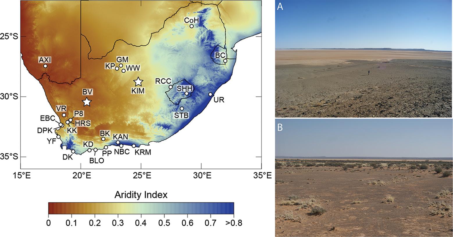
=Blombos
BC=Border Cave; BK=Buffelskloof; CoH=Cave of Hearths; DK=Die Kelders; DPK=Diepkloof; EBC=Elands Bay Cave; GM= Ga-Mohana Hill North; HRS=Hollow Rock; KRM=Klasies River; KK=Klein Kliphuis; KD=Klipdrift; NBC=Nelson Bay Cave; PP=Pinnacle Point; P8= Putslaagte 8; RCC=Rose Cottage Cave; SHH=Sehonghong; STB= Strathalan B; UR=Umhlatuzana; VR=Varsche Rivier; WW=Wonderwerk; YF=Ysterfontein; KP=Kathu pan. The key locales investigated by Carr et al.13 are shown (stars) (KIM= Kimberley and BV=Brandvlei). The photos of sites considered in this work show: (A) the margins of Hoek van Spruit se Vloer pan, south of Brandvlei, which exhibits varying densities of Middle and Later Stone Age lithic scatters around its margins (where the figure is standing); (B) the margins of Verkeerdevlei pan, southeast of Vanwyksvlei. Here the dark stoney surface in the foreground and middle ground is composed of abundant patinated artifacts, including diagnostic Middle Stone Age elements.
finding fish and crab remains during early 20th century quarrying.19 In all cases, the likely ages of these deposits and landforms were weakly constrained. The new work first sought to address their ages through the application of radiocarbon and optically stimulated luminescence (OSL) dating methods. However, it was also able to identify additional sites with evidence pertinent to these questions; notably the presence of freshwater mussel deposits at pans that are today very rarely inundated. The application of OSL dating was particularly significant as this method could provide numerical ages for deposits that were devoid of organic matter or biogenic calcite (e.g. shell).
Quantifying hydrological and ecological change
The results suggested the presence of perennial waters in the western arid interior at 55–39 ka, 34–31 ka and around 21 ka.13 In the east of the study region, at Kimberley, the age of a previously hypothesised20 44 km2 palaeo-lake was constrained to 25–32 ka; burial of these lake deposits by unambiguously Holocene age (10–11 ka) terrestrial colluvium further supported the notion that the cooler phases of the last glacial cycle were associated with a substantially different hydrological balance (i.e. ratio of evaporation to precipitation) from the present. A key development of this work was to move beyond dating phases of ‘higher’ moisture availability to develop a model that could account more specifically (i.e. climatically) for the hydrological changes implied by the geological evidence. By anchoring the model to the new geological data, we also sought to extend the findings to consider the implications for regional hydrology. For this we used the Shetran hydrological model21 to simulate surface water as well as soil water and groundwater flow (Figure 2). The modelling implied that significant hydrological invigoration across much of the Orange River catchment would have been required to sustain these lakes, with the most dramatic changes in water balance in the west. Temperature change (lower temperatures leading to lower evaporation rates) was likely to have been an important control, but increased rainfall was also needed to fully replicate the geological evidence. In the Brandvlei region, this amounted to potential evapotranspiration being reduced to 21% of present and rainfall increasing to 215% of present (to approximately 550 mm per year). A landscape of presently dry pans and ephemeral river channels was thus at times associated with perennial rivers and lakes and the regional water
table would have intersected the modern landscape across stretches of this interior region (Figure 2). Modelling also facilitates the development of testable hypotheses; if water resources were an important control on human occupation of the interior, the outputs offer suggestions in terms of where to look for new archaeological evidence.
In water-limited ecosystems, once the regional hydrology changes, ecological changes will follow, and using the modelling results, it was possibletodevelophypothesesastotheassociatedvegetationresponses. Crucially, the likely response of herbivores to these new conditions could also be considered. Here the modelling predicts a wetter, grassier and more herbivore-rich environment; a much more resource-rich landscape that would have presented many opportunities for hunter-gatherer communities.13 Indeed, there is independent faunal evidence to support these proposed changes22, and the results also explain some intriguing (but rarely discussed) elements of the Pleistocene faunal record; notably the presence of aquatic mammals like hippos (Hippopotamus amphibius), and lechwe (Kobus leche) which feed on aquatic plants, in several late Pleistocene faunal records in the arid interior.22
Implications and future perspectives
Considering this evidence, a parsimonious explanation for the archaeological ‘gap on the map’ (Figure 1) in the arid interior is not one of unfavourable (palaeo)climates, but more likely a reflection of geology and geomorphology. That is, the landscape is (was) unsuited to the preservation of the sorts of stratified archaeological records that have attracted intensive research efforts elsewhere. It is worth noting that where such sites are located in the interior, such as Wonderwerk Cave, Ga-Mohana Hill and Kathu Pan to the north of the aforementioned lake study sites, Early Stone Age, MSA and LSA archaeology, including some early MSA materials dating to the penultimate glacial period (Marine Isotope Stage 6), are indeed preserved.14,15,23
While unstratified, there is abundant surface archaeological evidence for hunter-gatherers in the interior region. The question of whether, at a regional scale, this is consistently concentrated around (palaeo) hydrological systems24 requires more work, but Carr et al.13 describe both MSA and LSA materials at all of their sampled/observed sites (Figure 1).
Volume 120| Number 3/4 March/April 2024 14 https://doi.org/10.17159/sajs.2024/17569 Invited Commentary Palaeohydrology and archaeology of the South African arid zone Page 2 of 4
Figure 1: The distribution of major Middle Stone Age sites (some sites also include Early and Later Stone Age materials) in South Africa with a map of aridity (aridity index calculated with data from Trabucco and Zomer6). AXI=Apollo 11; BLO
Cave;
Source: Carr et al.13, reproduced under a CC-BY-NC-ND 4.0 licence
Source:
The situation is thus idealised rather than actual, but sites for which direct field evidence for palaeolakes and perennial surface water flow has been identified are also shown (GV = Grootvloer; SKV = Swartvolkvloer;
Volume 120| Number 3/4 March/April 2024 15 https://doi.org/10.17159/sajs.2024/17569 Invited Commentary Palaeohydrology and archaeology of the South African arid zone Page 3 of 4
Figure 2: The results of the Shetran modelling, showing the modelled depth of the water table across the Orange River catchment for several potential evapotranspiration (PET) scenarios; white and blue shading indicates the water table intersection with the modern ground surface.13 It is important to consider that the size and climatic heterogeneity of the region depicted means that it is unlikely that all of it ever experienced precisely the same water balance or level of potential evapotranspiration.
AF = Alexandersfontein).
Carr et al.13, reproduced under a CC-BY-NC-ND 4.0 licence
At Alexandersfontein the density reaches greater than 50 artefacts/m2 at one locale on the edge of the proposed palaeo-lake.13,20 Here MSA artefacts were also found in stratified deposits, although age constraints for these materials are required. Looking further afield, it is clear that several pan sites, while lacking obvious shoreline deposits, were also associated with abundant MSA lithic scatters, and this includes some sites for which the hydrological modelling predicts palaeo-inundation (Figure 2). The role of springs in shaping landscape usage should also be considered.12
Thus, one might wonder to what extent our collective views on South African deep history are skewed by the stark nature of the modern conditions in the arid zone, and by a research focus on deeply stratified archaeological sites on the coastal margins. A growing body of work is developing around this issue, including the description and dating of new sites such as Ga-Mohana15 and work further afield in the Makgadikgadi Basin of Botswana25. More broadly, these works prompt us to consider the significance and potential of the interior surface archaeological record. The importance (and acknowledged challenges) of integrating surface archaeology into our wider understanding of human history is recognised globally, but the results discussed here suggest there is value in considering how the interior’s open-air record of human existence can be integrated into a broader understanding of South Africa’s past.26 Given its very emplacement within the landscape, if its chronological hurdles can be overcome, this surface archaeological record has the potential to deliver new behavioural information. That it spans a wider temporal and spatial range than rock shelter sites, moreover, and captures a broader range of activities and behaviours27, makes it all the more enticing. Crucially, though, to interpret the interior’s archaeology properly, and to fully grasp its strengths and limitations, we must also start to understand the geomorphic processes that shape surface archaeology.28 Doing so may be nothing short of the key to understanding when, why and how humans inhabited these perennial – but not permanent – thirstlands.
references
1. Mitchell P. The archaeology of southern Africa. Cambridge: Cambridge University Press; 2002.
2. Van Zinderen Bakker EM. The evolution of late Quaternary paleoclimates of southern Africa. Palaeoecol Afr. 1976;9:160–202.
3. Chase BM, Harris C, De Wit MJ, Kramers J, Doel S, Stankiewicz J. South African speleothems reveal influence of high- and low latitude forcing over the past 113.5 k.y. Geology. 2021;49(11):1353–1357. https://doi.org/10.1 130/G49323.1
4. Talma AS, Vogel J. Late Quaternary paleotemperatures derived from a speleothem from Cango Caves, Cape Province, South Africa. Quat Res. 1992;37(2):203–213. https://doi.org/10.1016/0033-5894(92)90082-T
5. Chase B, Meadows M. Late Quaternary dynamics of southern Africa’s winter rainfall zone. Earth Sci Rev. 2007;84(3–4):103–138. https://doi.org/10.101 6/j.earscirev.2007.06.002
6. Trabucco A, Zomer R. Global aridity index and potential evapo-transpiration climate database v2 [database on the Internet]. CGIAR-CSI; 2019. Available from: https://csidotinfo.wordpress.com/2019/01/24/global-aridity-index-an d-potential-evapotranspiration-climate-database-v2/
7. Butzer KW. Archeogeology and Quaternary environment in the interior of Southern Africa. In: Klein RG, editor. Southern African prehistory and paleoenvironments. Boca Raton, FL: CRC Press; 1984. p. 1–64.
8. Beaumont P. Where did all the young men go during 18O stage 2? Palaeoecol Afr. 1986;17:79–86.
9. Kent LE. Diatomaceous deposits in the Union of South Africa, with special reference to Kieselguhr. Geological Survey of South Africa Memoirs, 1947;42.
10. RobertsP,StewartBA.Definingthe‘generalistspecialist’nicheforPleistocene Homo sapiens. Nat Hum Behav. 2018;2(8):542–550. https://doi.org/10.1038 /s41562-018-0394-4
11. Deacon J. Patterning in the radiocarbon dates for the Wilton/Smithfield complex in southern Africa. S Afr Archaeol Bull. 1974;29:3–18. https://doi .org/10.2307/3887932
12. Sampson C, Moore V, Bousman C, Stafford B, Giordano A, Willis M. A GIS analysis of the Zeekoe Valley Stone Age archaeological record in South Africa. J Afr Archaeol. 2015;13(2):167–185. https://doi.org/10.3213/2191-5784-1 0277
13. Carr A, Chase B, Birkinshaw S, Holmes P, Rabumbulu M, Stewart B. Paleolakes and socioecological implications of last glacial “greening” of the South African interior. Proc Natl Acad Sci USA. 2023;120(21), e2221082120. https://doi.org/10.1073/pnas.2221082120
14. Chazan M, Berna F, Brink J, Ecker M, Holt S, Porat N, et al. Archeology, environment, and chronology of the Early Middle Stone Age component of Wonderwerk Cave. J Paleolit Archaeol. 2020;3:302–335. https://doi.org/10. 1007/s41982-020-00051-8
15. Wilkins J, Schoville BJ, Pickering R, Gliganic L, Collins B, Brown KS, et al. Innovative Homo sapiens behaviours 105,000 years ago in a wetter Kalahari. Nature. 2021;592(7853):248–252. https://doi.org/10.1038/s41586-021-03 419-0
16. Von Der Meden J, Pickering R, Schoville BJ, Green H, Weij R, Hellstrom J, et al. Tufas indicate prolonged periods of water availability linked to human occupation in the southern Kalahari. PLoS ONE. 2022;17(7), e0270104. http s://doi.org/10.1371/journal.pone.0270104
17. Partridge TC, Scott L, Hamilton JE. Synthetic reconstructions of southern African environments during the Last Glacial Maximum (21–18 kyr) and the Holocene Altithermal (8–6 kyr). Quat Int. 1999;57:207–214. https://doi.org/1 0.1016/S1040-6182(98)00061-5
18. Klein RG, Avery G, Cruz-Uribe K, Halkett D, Parkington JE, Steele T, et al. The Ysterfontein1MiddleStoneAgesite,SouthAfrica,andearlyhumanexploitation of coastal resources. Proc Natl Acad Sci USA. 2004;101(16):5708–5715. https://doi.org/10.1073/pnas.0400528101
19. Kent LE, Gribnitz KH. Freshwater shell deposits in the northwestern Cape Province: Further evidence for a widespread wet phase during the late Pleistocene in southern Africa. S Afr J Sci. 1985;81(7):361–370.
20. Butzer KW, Fock GJ, Stuckenrath R, Zilch A. Palaeohydrology of late Pleistocene Lake, Alexandersfontein, Kimberley, South Africa. Nature. 1973; 243(5406):328–330. https://doi.org/10.1038/243328a0
21. Birkinshaw SJ, James P, Ewen J. Graphical user interface for rapid set-up of SHETRAN physically-based river catchment model. Environ Modell Softw. 2010;25(4):609–610. https://doi.org/10.1016/j.envsoft.2009.11.011
22. Klein RG, Cruz-Uribe K, Beaumont PB. Environmental, ecological, and paleoanthropological implications of the late Pleistocene mammalian fauna from Equus Cave, Northern Cape Province, South Africa. Quat Res. 1991;36(1):94–119. https://doi.org/10.1016/0033-5894(91)90019-2
23. Beaumont P, Vogel J. On a timescale for the past million years of human history in central South Africa. S Afr J Sci. 2006;102(5/6):217–228.
24. Butzer KW. A “marginality” model to explain major spatial and temporal gaps in the Old and New World Pleistocene settlement records. Geoarchaeology. 1988;3(3):193–203. https://doi.org/10.1002/gea.3340030303
25. Burrough SL, Thomas DS, Allin JR, Coulson SD, Mothulatshipi SM, Nash DJ, et al. Lessons from a lakebed: Unpicking hydrological change and early human landscape use in the Makgadikgadi Basin, Botswana. Quat Sci Rev. 2022;291, Art. #107662. https://doi.org/10.1016/j.quascirev.2022.107662
26. Hallinan E. Landscape-scale perspectives on Stone Age behavioural change from the Tankwa Karoo, South Africa. Azania. 2021;56(3):304–343. https:// doi.org/10.1080/0067270X.2021.1960675
27. Mackay A. Three arcs: Observations on the archaeology of the Elands Bay and northern Cederberg landscapes. South Afr Humanit. 2016;29(1):1–5.
28. Fanning PC, Holdaway SJ, Rhodes EJ, Bryant TG. The surface archaeological record in arid Australia: Geomorphic controls on preservation, exposure, and visibility. Geoarchaeology. 2009;24(2):121–146. https://doi.org/10.1002/ge a.20259
Volume 120| Number 3/4 March/April 2024 16 https://doi.org/10.17159/sajs.2024/17569 Invited Commentary Palaeohydrology and archaeology of the South African arid zone Page 4 of 4
AuthorS:
Robyn Pickering1
Dipuo W. Kgotleng2
AFFILIAtIoNS:
1Department of Geological Sciences, Human Evolution Research Institute, University of Cape Town, Cape Town, South Africa
2Palaeo-Research Institute, University of Johannesburg, Johannesburg, South Africa
CorrESPoNDENCE to:
Robyn Pickering
EMAIL:
robyn.pickering@uct.ac.za
hoW to CItE:
Pickering R, Kgotleng DW. Preprints, press releases and fossils in space: What is happening in South African human evolution research? S Afr J Sci. 2024;120(3/4), Art. #17473. https://doi.org/10.17159/sajs.202 4/17473
ArtICLE INCLuDES:
☐ Peer review
☐ Supplementary material
KEYWorDS:
preprints, human evolution, Homo naledi, hominin fossils, ethical publishing
PubLIShED: 27 March 2024
Preprints, press releases and fossils in space: What is happening in South African human evolution research?
Significance:
Uploading unreviewed manuscripts to a preprint server promotes accessibility and facilitates rapid breakthroughs. We, however, question the motivation of Berger and colleagues who used the new eLife publishing model to launch what appeared to be a carefully curated media campaign around an unreviewed narrative, thereby manipulating accepted norms in scientific publishing. This team has engaged in ostentatious public displays under the guise of promoting science, including launching precious fossil remains into space. Given these ethical concerns, we call on the public, heritage and scientific practitioners to reflect on the current state, and future, of human evolution research.
2023 was a big, busy year for the field of human evolution research, or palaeoanthropology, in South Africa – it attracted headlines, debate and controversy. The focus is the Rising Star Cave system, within the UNESCO Cradle of Humankind World Heritage Site, known as the Cradle, which is home to the fossil remains of our distant relative, Homo naledi. The Cradle has produced much of what we know about early human evolution and its cave sites are the single richest collection of early human, or hominin, fossils anywhere on earth. The caves and fossils of this region have been the subject of research, debate and media interest for almost a century. But 2023 marked a departure from what is considered normal in even this oft acrimonious, competitive research field.
On 5 June 2023, three multi-authored manuscripts were posted as pre-prints on the bioRxiv server, by a team led by Lee Berger.1-3 These manuscripts had been submitted previously to the online only journal eLife and were sent for peer review on 4 May 2023. The posting on the preprint server a month later was done in accordance with the new eLife open publishing model, launched in March 2023.4
There followed a huge, coordinated, and thorough media coverage of not the actual manuscripts but the central, as yet unreviewed, narrative that Homo naledi had buried their dead, and made art and stone tools. The news reverberated around the world, with headlines on CNN, The New York Times, National Geographic and beyond. This was accompanied by a blitz of media interviews and television appearances by Berger. This gave the impression of a carefully planned and curated media exercise, with field photos, figures from the manuscripts and dramatic artistic reconstructions featured in online and print media.
Then on 12 July 2023, peer reviews of the three manuscripts were posted on the respective webpages of each preprint on the eLife system5; four reviews appeared each for Berger et al.1 and Berger et al.2, and three reviews appeared for Fuentes et al.3 Ten of these eleven independent peer reviews rejected the claims put forward in the three manuscripts. A subset of senior authors responded5, but are yet to revise the manuscripts. Five days later, on 17 July 2023, a Netflix documentary titled Unknown: Cave of Bones was released in 24 countries around the world, featuring the same narrative as the unreviewed manuscripts and initial media releases, that is, that Homo naledi had buried their dead, and made art and stone tools. This was followed in October 2023 by a book with a similar title.6 How did all of this happen? How could an unreviewed narrative enter the public realm in such a comprehensive way and then be almost unanimously rejected by peer review? The answer is eLife’s new publishing approach, and what we view as the deliberate exploitation of this model by the Berger et al. research team. eLife launched their new publishing model in March 2023.4 This model is a marked departure from the traditional model in which authors submit a manuscript and a journal editor either desk rejects or sends the manuscript for peer review. The editor then accesses the reviews and passes these back to the authors with the editorial decision to either reject or publish a revised version of the manuscript, with minor or major revisions. This has been the standard practice since the mid-1970s, as a measure of quality control and a means to improve the standard of scientific outputs. Only in rare cases is a manuscript accepted more or less as is; we emphasise this point: almost all manuscripts are subject to some level of revision prior to publication.
eLife states, in their own words, that while “authors still receive a high-quality peer-reviewed eLife publication” , their new model is different in two key ways.4 For clarity, we quote them directly: “Firstly, all papers that are invited for review are published on the eLife website as a Reviewed Preprint, giving readers an earlier view of the reviews and editor’s assessment. Secondly, the authors control the next steps. This can include submitting a revised preprint or publishing their Reviewed Preprint as a Version of Record which will be sent to indexers like PubMed and can be listed in funding, job applications and more.”
Our view is that these two key differences have been exploited by Berger et al. The requirement that the manuscripts be placed on a preprint server was satisfied, but the team then used this version of the manuscripts to launch their massive media announcement. In their later response to the eLife commissioned reviews5, the team disclose that they had “benefited from a previous round of review of the manuscript describing the proposed burial features, which underwent two rounds of revisions in a high-impact journal over a period of approximately 8 months during 2022 and early 2023”. The manuscript including the deliberate burial data set and accompanying narrative had been peer reviewed, and presumably rejected by a ‘high impact journal’ editor, meaning that the authors had an idea of how their interpretation was going to land with the scientific community. Then, rather than wait for a new set of
17 https://doi.org/10.17159/sajs.2024/17473 Volume 120| Number 3/4 March/April 2024 © 2024. The Author(s). Published under a Creative Commons Attribution Licence. Commentary
peer reviews, they chose to go ahead with the media campaign without having met peer review approval.
Immediately after the preprints were released, critical commentary emerged.7 The manuscripts were criticised by the reviewers, who wrote long, detailed, meticulous reviews of all aspects of the data, claims and interpretations. These reviews are all publicly available on the eLife site.5 The team responded to the reviews by thanking the reviewers but argued that they maintained their original interpretations, although they are yet to present a detailed scientific rebuttal of the criticisms, nor revise the manuscripts. This means that the original, unreviewed versions are taking the place of reviewed manuscripts and the authors, not the editors, are deciding what quality of research is considered acceptable.
There was very little media coverage of the peer-review reports and responses from the scientific community, compared with the huge media blitz around the preprints. Discussion on X (formerly Twitter) exploded with commentary and opinions; Nature covered the response to the reviews8, but the mainstream media that had disseminated the deliberate burial/art/tool narrative looked the other way when this interpretation was condemned by the scientific community.
The ‘Cave of Bones’ Netflix documentary soared to the top of the ‘most watched’inSouthAfricaintheweeksafteritfirstaired.Thisteamappeared to have moved beyond interpretation of their data, to create an entire narrative arc to explain their observations, without having been subject to the usual rigours of scientific publication. Indeed, they took deliberate steps to curate and promote their version before it was approved by the peer-review process. Filming an entire documentary is not a trivial exercise, and this piece was made, edited, scored and readied for release before the actual science had been reviewed, criticised, revised and taken its place within what the scientific community accepts as new knowledge. This is not just a muddle of dates, or a slip of the tongue at a stressful press interview by a media-shy academic. This appears to be a deliberate and well-planned exploitation of a new publishing model to shortcut the usual scientific process of academic publishing.
How did we get here? What are preprints, what is their normal role, and how is their use going to impact future research? These are important questions. As we are not experts on this topic, we offer up an explanation from the preprint server bioRxiv9: “Because this [sic traditional] process can be lengthy, authors use the bioRxiv service to make their manuscripts available as ‘preprints’ before certification by peer review, allowing other scientists to see, discuss, and comment on the findings immediately.” For other scientists to see, discuss and comment; not to orchestrate a press release and Netflix documentary.
The bioRxiv explanation continues: “Readers should therefore be aware that articles on bioRxiv have not been finalized by authors, might contain errors, and report information that has not yet been accepted or endorsed in any way by the scientific or medical community.” This is a very clear and precise warning that places the preprints into the context in which they should be used and makes clear how they are intended to be viewed. There is also no ambiguity about how these preprints should be used by the media; bioRxiv cautions, “We also urge journalists and other individuals who report on medical research to the general public to consider this when discussing work that appears on bioRxiv preprints and emphasize it has yet to be evaluated by the medical community and the information presented may be erroneous.” None of this caution was mentioned in the media coverage nor the Netflix film.
What we saw unfold in 2023 is the intersection of an established publishing norm in some fields (preprints) and a research team that has sought to disseminate a singular, interpretative narrative prior to peer review. Preprints per se are not the issue here – posting unreviewed research on a preprint server is not new or controversial; we saw during the pandemic that this was useful and productive, and how research on treatments for COVID-19 and vaccine development could proceed very quickly when aided by the sharing of results and open reviews.
But palaeoanthropology is not a field that needs urgent research and rapid breakthroughs. Given the huge and wide public interest in human
evolution and our origins, this research field benefits from much slower, measured, and careful research. The Cradle has produced an invaluable fossil record, and the Rising Star Cave is no different. The puzzle of how so many fossil bones of a small-brained hominin ended up in a now inaccessible chamber of a deep underground cave system is an intriguing question. A slow, rigorous, traditional approach to researching this cave and its associated fossils will yield exciting new results; there is no demonstrable need to peddle an unreviewed narrative to the public.
June and July 2023 were eventful and controversial months for palaeoanthropology research and publishing in South Africa. Surely no one could have anticipated what followed just two months later. Berger, with the permission of the South African Heritage Resource Agency (SAHRA)10 and the curating institute responsible for the Cradle fossils, the Evolutionary Studies Institute at the University of the Witwatersrand11 , sent a thumb bone of Homo naledi and a fragment of the collar bone of Australopithecus sediba, into space. These two fossils were placed in a custom-made carbon-fibre tube and carried by billionaire Tim Nash, who was a passenger on the Virgin Galactic space flight on 8 September 2023, and is also a landowner in the Cradle.10,11
The reason given in the request for temporary export of the fossils out of South Africa by Berger was “to promote South African science”10 However, the media coverage of the fossil spaceflight was even more focused on an American audience than the June preprint splash. Coverage by the South African media, a week later, focused on the outrage of both local and international scientists12-14 who argued that this endeavour had little scientific merit and was a publicity stunt. As if palaeoanthropology in South Africa had not suffered enough reputational damage, this took place during the month of September, Heritage Month in South Africa, during which we reflect on, celebrate and honour our heritage.
This space flight takes us into murky waters, raising questions of ethics such as ‘whose heritage is this anyway?’ and questioning why privileged people can take fossils to space for no valid reason, while the poor communities from where the fossils originate are excluded from even talking about how they could benefit from accessing the material.14 We are referring to the case of the local community at Taung in the Northern Cape and their repeated requests for not only access but for a return of the ‘Taung child’ fossil to the town.15
While it feels like this surely must be the end of this story, it is not. On 10 November 2023, a peer-reviewed article was published in the Journal of Human Evolution titled ‘No scientific evidence that Homo naledi buried their dead and produced rock art’ in which Martinón-Torres et al.16 systematically dismantle every aspect of the three preprints and argue convincingly that the evidence provided by Berger and his team in no way supports their interpretations. There was some media coverage of this article and the reaction to it, but, again, not on the same scale as that of the June coverage.
So, looking back at an eventful 2023, we are left with more questions than answers. Is the media narrative and a fascinating story more important than peer review? Are we looking at sensational documentary films setting the pace, tone and quality of South African research into human origins? Are some claiming to promote South African science actually doing more harm than good? Are our precious, rare fossils being used to promote individual agendas with disregard for the risks? Is it not our academic responsibility to entrench our work, and especially public engagement initiatives, in scientific integrity?
In our view, the answer to all these questions is yes. We end with a final question for the South African palaeoscience, and broader research, community: Is this what we want? We call on this community, as well as on the funders, heritage practitioners, permit granting agencies, and government research bodies, to take a long hard look at human evolution research and its associated disciplines in 2023 and consider where we want to be in 2024 and beyond.
Competing interests
We have no competing interests to declare.
Volume 120| Number 3/4 March/April 2024 18 https://doi.org/10.17159/sajs.2024/17473 Commentary Fossils in space, press and South African human evolution research Page 2 of 3
references
1. Berger LR, Hawks J, Fuentes A, van Rooyen D, Tsikoane M, Ramalepa M, et al. 241,000 to 335,000 years old rock engravings made by Homo naledi in the Rising Star Cave system, South Africa [preprint]. bioRxiv. 2023:2023.06.01.543133. https://doi.org/10.1101/2023.06.01.543133
2. BergerLR,MakhubelaT,MolopyaneK,KrügerA,Randolph-QuinneyP,ElliottM, et al. Evidence for deliberate burial of the dead by Homo naledi. bioRxiv. 2023:2023.06.01.543127. https://doi.org/10.1101/2023.06.01.543127
3. Fuentes A, Kissel M, Spikins P, Molopyane K, Hawks J, Berger LR. Burials and engravingsinasmall-brainedhominin, Homo naledi,fromthelatePleistocene: Contexts and evolutionary implications. bioRxiv. 2023:2023.06.01.543135. https://doi.org/10.1101/2023.06.01.543135
4. eLife. eLife’s NEW Model: Your questions answered [webpage on the Internet]. c2023 [cited 2023 Nov 29]. Available from: https://elifesciences.or g/inside-elife/2b765a27/elife-s-new-model-your-questions-answered
5. Anonymous Reviewers. Reviews of Berger et al. c2023. [cited 2023 Nov 29]. https://doi.org/10.7554/eLife.89106.1
6. Berger LR, Hawks J. Cave of bones: A true story of discovery, adventure, and human origins. Johannesburg: Penguin Random House; 2023.
7. Petraglia M, Ndiema E, Martinón-Torres M, Boivin N. Major new research claims smaller-brained Homo naledi made rock art and buried the dead. But the evidence is lacking. The Conversation. 2023 June 06. [cited 2023 Nov 29]. Available from: https://theconversation.com/major-new-research-claim s-smaller-brained-homo-naledi-made-rock-art-and-buried-the-dead-but-th e-evidence-is-lacking-207000
8. Callaway E. Sharp criticism of controversial ancient-human claims tests eLife’s revamped peer-review model. Nature News. 2023 July 25 [cited 2023 Nov 29]. https://doi.org/10.1038/d41586-023-02415-w
Fossils
9. bioRxiv. Frequently asked questions (FAQ) [webpage on the Internet]. No date [cited 2023 Nov 29]. Available from: https://www.biorxiv.org/about/FAQ#un refereed
10. Berger LR. Hominin space flight: SAHRIS [webpage on the Internet]. c2023 [cited 2023 Nov 29]. Available from: https://sahris.sahra.org.za/node/621314
11. NewsWR.Firstfossilsofancienthumanrelativesjourneytospace–University of the Witwatersrand [webpage on the Internet]. c2023 [cited 2023 Nov 29]. Available from: https://www.wits.ac.za/news/latest-news/research-news/20 23/2023-09/first-fossils-of-ancient-human-relatives-journey-to-space.html
12. Callaway E. Ancient-human fossils sent to space: Scientists slam ‘publicity stunt’. Nature News. 2023 September 13 [cited 2023 Nov 29]. Availablefrom: https://www.nature.com/articles/d41586-023-02882-1
13. Professor Lee Berger owes SA an apology. Questions need to be asked about whether any money changed hands. 2023 September 21 [cited 2023 Nov 28]. Available from: https://www.citizen.co.za/news/opinion/professor-lee-b erger-owes-sa-an-apology/2023
14. Kgotleng DW, Pickering R. South African hominin fossils were sent into space and scientists are enraged. The Conversation Africa. 2023 [cited 2023 Nov 28]. Available from: https://theconversation.com/south-african-hominin-foss ils-were-sent-into-space-and-scientists-are-enraged-213818
15. Maje O. Locals want Taung Skull returned home. Sunday World. 2022 March 07 [cited 2023 Nov 28]. Available from: https://sundayworld.co.za/news/loc als-want-taung-skull-returned-home
16. Martinón-TorresM,GarateD,HerriesAIR,PetragliaMD.Noscientificevidence that Homo naledi buried their dead and produced rock art. J Hum Evol. 2023, Art. #103464. https://doi.org/10.1016/j.jhevol.2023.103464
Volume 120| Number 3/4 March/April 2024 19 https://doi.org/10.17159/sajs.2024/17473 Commentary
Page
of 3
in space, press and South African human evolution research
3
AuThor:
Brian A. Austin1
AFFILIATIoN:
1Retired Engineering academic, University of Liverpool, Liverpool, UK
CorrESPoNDENCE To:
Brian Austin
EMAIL:
abkaustin@aol.com
hoW To CITE:
Austin BA. Radio communications through rock strata – South African mining experience over 50 years.
S Afr J Sci. 2024;120(3/4), Art. #17301. https://doi.org/10.17159/sa js.2024/17301
ArTICLE INCLuDES:
☐ Peer review
☐ Supplementary material
KEYWorDS:
radio communications, mining, rock strata, handheld radio
PubLIShED: 27 March 2024
Radio communications through rock strata – South African mining experience over 50 years
Significance:
The pioneering work done in South Africa in developing radio communications technology for use underground in mines is summarised. Propagation took place, in the main, directly through the rock strata with incidental coupling into power cables, pipes, rails and other conductors. The research established the optimum frequencies for communications as well as the most appropriate antennas. Specialised radio equipment was developed for this task as constrained by the technology of the time. Size and weight were major constraints; ultimately, handheld equipment, using single-sideband modulation, was produced that functioned exceptionally well in numerous situations underground.
Introduction
It was early in 1938 that the medical superintendent of Rand Mines, Dr A.J. Orenstein, asked Professor Basil Schonland, the Director of the Bernard Price Institute of Geophysical Research (the BPI) at the University of the Witwatersrand, about the feasibility of radio communications underground in mines. Orenstein had long been concerned that firefighting and rescue teams were severely hampered by a lack of communication between those personnel and anyone else when they ventured into the most hazardous of situations. Schonland was sceptical that radio signals would propagate over useful distances through rock strata, but agreed to investigate.1,2
The war, radar and the Special Signals Services
International events soon intervened as war with Nazi Germany loomed. South Africa declared war on 6 September 1939, just three days after Britain. From then, the research focus of the BPI shifted inexorably. Henceforth, all its resources, as limited as they were, would be given over to the investigation of RDF, or radar as it was known in those earliest days (see Figure 1). What followed, was the formation of the Special Signals Services (SSS), as part of the South African Army’s Corps of Signals with Lt Col Schonland as its commanding officer.2,3 And immediately, the SSS co-opted the services of engineers and physicists from South Africa’s major universities – one of whom was a young engineering graduate from Durban by the name of Trevor Wadley.
The development of South Africa’s own radar equipment and its deployment, along with subsequent British radars, around the country’s coastline as well as in East Africa, the Middle East and in Italy, has been reported extensively elsewhere.2-4 It was that massive wartime effort at the BPI that was the spur to the formation of the Council for Scientific and Industrial Research (CSIR), which was formally established in October 1945 with Schonland as its President. And the CSIR’s first specialist laboratory to come into existence was the Telecommunications Research Laboratory, with Wadley among its first members of staff.5
Wadley and radio underground
Wadley’s genius was soon evident. He designed a revolutionary type of radio receiver that became the mainstay of British naval communication when the equipment was produced by a British company. Subsequently, he developed
20 https://doi.org/10.17159/sajs.2024/17301 Volume 120| Number 3/4 March/April 2024 © 2024. The Author(s). Published under a Creative Commons Attribution Licence. Commentary
Figure 1: The mobile radar system designed and constructed by the Special Signals Services at the Bernard Price Institute of Geophysical Research, University of the Witwatersrand, in 1942.
a distance-measuring device of quite unparalleled accuracy called the Tellurometer which revolutionised the field of surveying.5,6 Remarkably, he also turned his attention to the problem of radio communications in mines that had first been raised almost a decade before.
In 1949, Wadley wrote a report for the Transvaal and Orange Free State Chamber of Mines describing the outcome of his research and his recommendations for suitable equipment.7 The important question he answered was what the optimum frequency was in order to achieve maximum communication range directly through the rock. Reliance could not be placed on signals propagating via the underground tunnels because of their irregular shapes, their curvature and roughness, which ruled out line-of-sight communications.
Electrical properties of rocks
In order to determine how electromagnetic energy might propagate through the lossy dielectric medium of rock, one requires a knowledge of its propagation constant γ where:
γ = α + jβ = √jωμ(σ + jωϵ)
Here α is the attenuation constant, β is the phase constant and ω = 2πf is the angular frequency. The other terms are the fundamental electrical parameters of rock: its conductivity (σ), dielectric constant (ε) and magnetic permeability (μ). Of these, only the permeability remains constant with changes in frequency, while most geological materials are also non-magnetic.8 By contrast, both rock conductivity and dielectric constant are frequency dependent.8,9
Wadley measured both the resistivity (the reciprocal of conductivity) and the dielectric constant of quartzite and some shales typical of the gold mining region of the Witwatersrand. He used borehole samples with apparatus specially designed for the task. In his report he showed how the resistivity of quartzite varied from about 9 × 10⁴ to 5 × 10³ ohmmetres over a frequency range from 100 kHz to 3 MHz. By contrast, the dielectric constant hardly changed and had a value of about 6. Using these data, he calculated the attenuation of a radio signal propagating through 300 m of quartzite and showed how it increased rapidly with frequency, implying that the lower the radio frequency, the better for communicating through rock.
Antennas in lossy media
The fact that the antennas would be surrounded by rock complicated the situation considerably. Wadley considered that a long centre-fed dipole antenna laid along the tunnel floor, or footwall, would be an appropriate antenna for a fixed station underground. For the portable equipment he chose a frame aerial which is essentially a loop of wire (perhaps of many turns) that would be wound around a miner’s helmet or ‘hardhat’. He measured the impedance of the dipole at a particular frequency and attributed the results to the electrical characteristics of the surrounding rock. From those measurements he deduced the antenna’s loss from 10 kHz to 10 MHz. As expected, there was a trade-off, between the rock-induced loss and the improved performance of the antenna as its apparent length, relative to the wavelength, increased with frequency.7
By contrast, the small loop antenna was difficult to treat theoretically because the interchange of energy between the air-space and rock was not well understood. This was undoubtedly true and it was to be many years before the underlying electromagnetics principles affecting such electrically small antennas, when immersed in lossy dielectric media, were fully explained.10,11
The optimum frequency
Wadley produced a graph of the total loss in decibels (dB) suffered by a radiating signal over a distance of 900 m for frequencies between 30 kHz and 3000 kHz. The graph went through a distinct minimum at about 300 kHz, which, therefore, is the optimum transmitting frequency for that particular distance. The graph also showed that for communications over greater distances a lower frequency would be required, while a higher frequency could be used over shorter distances.7
As in all radio communication systems, it is not just the strength of the signal that determines optimum performance but rather the signal-tonoise ratio. A deep-level mine presents an almost unique environment from a noise point of view. The great thickness of the overburden removes, almost completely, any electrical noise generated above ground (including by lightning) and therefore the only noise will be that caused by nearby electrical equipment and within the radio receiver itself. In the case of mining emergencies, all electrical power is usually switched off in the affected area, leaving just the receiver-generated noise which can be reduced substantially by careful design.7
The radio equipment
Wadley recommended that two types of transmitters be developed: a static set, producing about 4W of power to be used at a fixed point underground where it could make use of a fairly long antenna; and a portable set, generating only a tenth of the power and using a considerably smaller antenna. Naturally, each transmitter had its companion receiver, with each being of a modern superheterodyne configuration for optimum performance. Based on those specifications, he predicted that the normal operating radius would be about 600 m. A workable signal should still be received at a distance of around 750 m, while the absolute limit would be about 900 m. An appropriate transmitting frequency should be about 350 kHz.7
Because the radio technology of those days was all based on thermionic valves, the equipment would naturally be rather bulky. Wadley estimated that the larger unit would weigh no more than 14 kg, while its portable counterpart might be about a third of that.
Wadley never published his results in the open literature. This was an unfortunate omission because there was a real dearth of such quantitative data at that time.10
An industrial hiatus and a mining catastrophe
It was not until the late 1950s, on the formation of what was to become the research laboratories of the Chamber of Mines, that Wadley’s recommendations received serious attention from the South African mining industry. The problems foreseen by Dr Orenstein all those years before had by no means gone away: if anything, the expansion of the postwar gold and coal mining industries, and the stepped-up production then taking place, had exacerbated the problem of underground fires, accidents and, of course, the ever-present risk of rock falls at the increasing depths at which gold was being mined. On 21 January 1960, a disaster occurred at Coalbrook Colliery in the northern Free State when the mine workings collapsed, entombing 435 men, all of whom perished. Immediate attempts to rescue them were set in train with the Mines’ Rescue Brigade of 250 men leading the effort. These highly trained personnel were all experienced miners who had volunteered for the dangerous task of firefighting and rescue work underground. They were trained at the Chamber’s Rescue Training Station in Johannesburg.12 However, once they went underground, those rescue teams were without any form of communication.
Designing the equipment
The underground radio project had been resurrected by the Electronics Division of the Chamber’s laboratories during the late 1950s. Wadley’s findings and recommendations underpinned their work. Their own calculations had confirmed that a system loss of 150 dB between transmitter and receiver was tolerable and the family of curves in Figure 2 indicated the optimum frequencies for particular distances between them.13
Despite the decade or so that had elapsed since the invention of the transistor, and its rapid embrace by many sectors of the electronics engineering industry, the germanium transistors of that era were still limited to low-frequency and relatively low-power applications. They were also thermally sensitive devices, which was an important consideration to be born in mind given the very high temperatures experienced in deep mines.
The radio equipment would be used by members of the Mines Rescue Brigade, known as ‘Proto teams’ because of the Proto breathing apparatus they used. It required its user to clench a snorkel-type
Volume 120| Number 3/4 March/April 2024 21 https://doi.org/10.17159/sajs.2024/17301 Commentary Radio communications through rock strata Page 2 of 7
breathing tube between their teeth and to wear a nose clip. Both made speech impossible. This restriction had a great bearing on the design of the radio equipment.
Standard practice during mine emergencies was to establish a so-called fresh-air base, as close as possible to the disaster area, where breathing
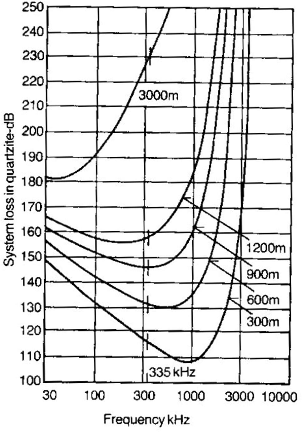
apparatus was not required. The Proto team, carrying the portable radio equipment, would then go forward from there to carry out its task.
An amplitude-modulated (AM) transmitter was designed for use at the fresh-air base. The frequency allocated by the Postmaster General for mining applications was 335 kHz. The transmitter’s output power was approximately 5 W. To exploit the very low noise conditions expected during a disaster, the receiver was designed to have the lowest possible noise figure. The base station weighed 13 kg. However, the motor car battery needed to power it weighed rather more at 15 kg.13
The portable equipment to be carried by a Proto team brigadesman was as small and light as possible within the constraints imposed by the valve technology of the time. It was intended to transmit a simple on-off code by means of a push-button because of the radio operator’s inability to speak. It was believed, quite rightly, that teaching everyone the Morse code was neither feasible nor necessary as long as a simple question and answer protocol was developed between the fresh-air base radio operator and his counterpart using the portable equipment. The portable transmitter, which resulted, produced about 2 W and its receiver also had the lowest possible noise figure. The portable set weighed just over 6 kg, including batteries.13
Loop antennas were used at both the fresh-air base and with the portable equipment. The base station antenna, shown in Figure 3, was a 1-m diameter multi-turn loop encapsulated in fibreglass and intended to be positioned horizontally on the ground. This orientation would ensure that it had all-round coverage, unlike the long length of wire intended by Wadley, which was markedly directional. The portable set, with its multiturn loop antenna contained within the rigid carrying harness, is shown in Figure 4. The receiver’s loudspeaker was mounted within the harness and positioned close to the operator’s ear.
underground trials
Numerous underground trials were conducted by the Chamber’s engineers. It soon became apparent that the communication ranges achieved were often considerably greater than those predicted by Wadley. The reason was that the signals were being conducted (and then re-radiated) by any cables, pipes and even the rails used by the electric and diesel-powered locomotives that transported men, materials and, of course, the gold-bearing rock throughout the mine.13
By contrast, in areas completely devoid of all conductors, communication range varied considerably, not only from mine to mine but also within a single mine. The reason, of course, was the complexity of the geology.
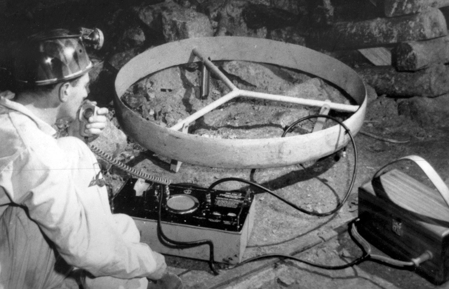
Volume 120| Number 3/4 March/April 2024 22 https://doi.org/10.17159/sajs.2024/17301 Commentary Radio communications through rock strata Page 3 of 7
Figure 2: Calculated system loss with frequency for various distances through quartzite rock.
Figure 3: The fresh-air base radio equipment, its battery and multi-turn loop antenna.

Extensive investigations carried out in subsequent years provided considerable insight into the propagation mechanisms involved through what was an inhomogeneous lossy dielectric medium, usually stratified and intersected by intrusions such as dykes. A most important theoretical analysis, carried out by J.R. Wait in the USA, provided the first detailed explanation of the phenomena.14 He showed that rock stratification can actually guide radio signals to greater distances than would be possible through a homogeneous medium. This would later be confirmed both in US coal mines and in South African gold mines.15 But, despite the progress made, it was clear that the equipment was too bulky and heavy.
A solid-state solution
In the late 1960s, the Chamber contracted a company in Cape Town to produce a compact, fully transistorised transceiver modelled on the packsets then coming into service with the armies around the world. Instead of a separate base station and a portable unit, a single piece of equipment could function in both roles, with the option to use a much bigger loop antenna when the equipment was set up at the fresh-air base. Single-sideband modulation instead of the AM would be used. For the same amount of transmitted power, single-sideband yields a 9 dB signalto-noise ratio advantage at the receiver. The equipment, as produced, operated at 335 kHz and is shown in Figure 5 along with its elliptical loop antenna. Being completely solid-state, it was considerably smaller and lighter than the previous valve-based hardware and contained its own rechargeable battery supply. The transmitter power output was increased to 10 W and the receiver, again, was as sensitive as possible. Once again, small multi-turn loops were used with the portable equipment with a larger, single-turn, flexible loop at the base station. Attention was also paid to ensuring that the equipment was ‘intrinsically safe’ so that it could be used in the flammable atmospheres typical of some mines.16
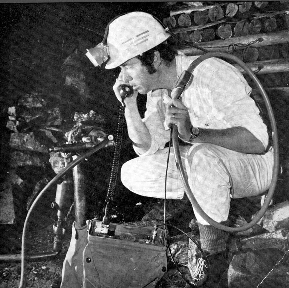
Once the prototypes had been evaluated and accepted by the Chamber’s Electronics Division, a company in Braamfontein, Johannesburg, was commissioned, in 1972, to manufacture a small quantity for further testing by the Rescue Training Station personnel. Word had by now reached the United States Bureau of Mines (USBM) about these South African developments and they purchased six transceivers for evaluation in US coal mines.15 Soon applications other than mining emergencies suggested themselves and the Chamber laboratories demonstrated the equipment’s usefulness for complex underground activities such as raise-boring and tramming as well as within the stopes adjacent to the reef being mined. One of those special projects was the Chamber’s Mining Technology Laboratory’s mechanised mining programme at Doornfontein Goldmine near Carletonville. There, more than 3000 m below the surface, multiple rock-cutting machines were undergoing evaluation and assessment. It was believed that good communication between the machine operators and the maintenance personnel would improve the efficiency of the process significantly. But the extremely cramped confines of a gold mine stope made even that packset-size equipment too unwieldy and so the need arose for something even smaller.
handheld communications
Examination of Figure 2 shows that a frequency close to 1 MHz could be used very effectively to communicate over a distance of 300 m through quartzite, with a considerable saving in transmitter power compared with 335 kHz. In addition, those experimental mechanised stopes were well served by armoured power cables and hydraulic lines. Tests had shown that this higher frequency propagated very effectively in and around the stopes, so an immediate design effort was mounted to produce a handheld transceiver.
The outcome was a single-sideband transceiver which weighed much less than a kilogram.16 It was called the TXR-1 and operated at 903 kHz for reasons of the novel technology used (Figure 6). The transmitter output power was 1 W. The antenna was a flexible multi-turn loop that fitted, bandolier style, around the miner’s body. The TXR-1 provided excellent two-way voice communications with a base station (using the same transceiver technology but with the addition of a 10-W power amplifier), plus a large loop antenna, erected in the storeroom close to the stope from where the whole operation was coordinated. More than a hundred TXR-1s in their canvas carrying pouches were produced over the following years to serve the rock-cutter stope.
Volume 120| Number 3/4 March/April 2024 23 https://doi.org/10.17159/sajs.2024/17301 Commentary Radio communications through rock strata Page 4 of 7
Figure 4: A brigadesman, using Proto breathing apparatus, with the portable radio equipment slung across his chest.
Figure 5: The single-sideband 335 kHz solid-state transceiver with its elliptical loop antenna.
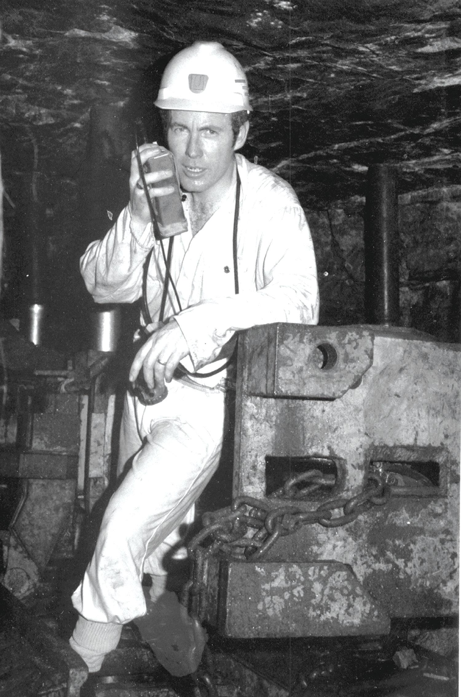
Commercial opportunities
The undoubted success of the TXR-1 had indicated that a more sophisticated small radio transceiver might well find applications throughout the mining industry. With this in mind, the Electronics Division set about developing a prototype which would embody stateof-the art electronic techniques. The intention was that it should operate from 100 kHz to 1 MHz in 10-kHz steps.17 Multiple mining activities all within the same relatively small area, if required, could then be accommodated on adjacent frequencies. Trials underground showed the hardware to be very acceptable, and so an approach was made to a commercial manufacturer of military-grade electronics equipment in Pretoria to customise it. The outcome was that, by 1978, the SCR-100
portable and SC-200 packset transceivers were available for sale to the mining industry. They immediately went into service with the Rescue Training Station (Figure 7) and in the rock-cutter stope. An energetic marketing exercise was then mounted by the manufacturer which resulted in many mines in South Africa, elsewhere in Africa and abroad, purchasing the equipment.17
An underground laboratory
The part played by power cables, water pipes and even rails in enhancing signal propagation was an undoubted fact, but the mechanisms involved were poorly understood. However, research in the USA and Europe had identified two possible modes of propagation known as the
Volume 120| Number 3/4 March/April 2024 24 https://doi.org/10.17159/sajs.2024/17301 Commentary Radio communications through rock strata Page 5 of 7
Figure 6: TXR-1
903 kHz handheld transceiver in a mechanised gold-mine stope.
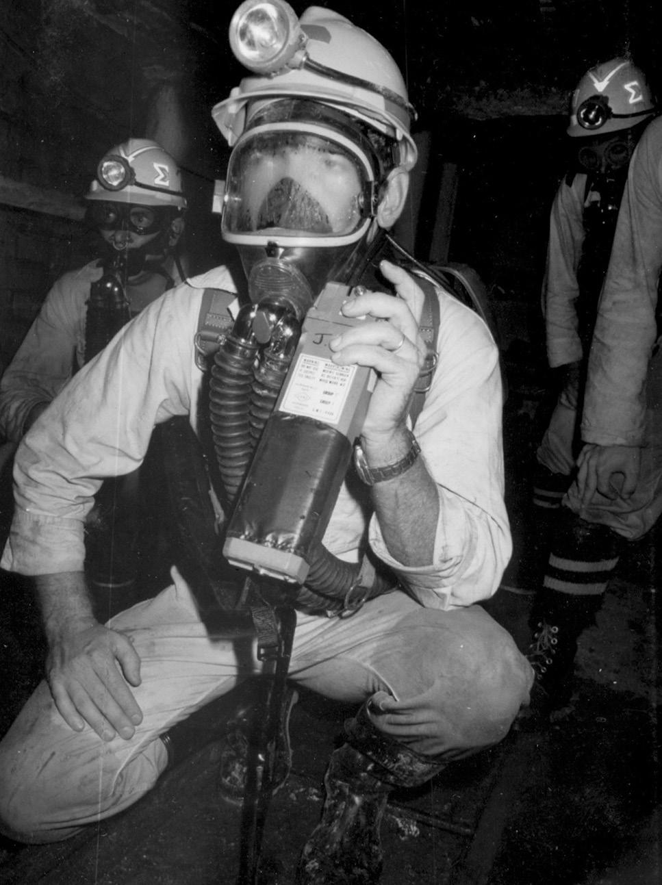
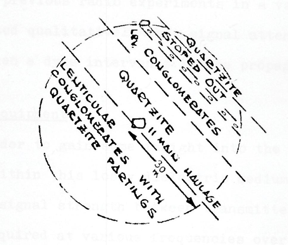
monofilar and bifilar modes.18 The details are beyond the scope of this Commentary, but suffice it to say that one or other of those modes can be used very effectively if the radio antennas are in fairly close proximity to those conductors. It was found that positioning a base station within an electrical sub-station, either underground or even on the surface, could yield really long-distance (>3000 m) radio communications by one or other of those modes.19
To investigate all the modes of propagation, an underground laboratory was required and a convenient site was found in a completely workedout area of a mine devoid of electrical conductors. The rock was predominantly quartzite but there was also considerable stratification both above and below the test area. It became apparent that the direction of the electric field polarisation affected the rate of signal attenuation. Maximum signal strength occurred when the antennas were tilted some 40 degrees to the horizontal. This implied that the strata of the surrounding rock were affecting propagation. Examination of a map (see Figure 8) showing the geology of the area confirmed that dip angle of the strata.17,20
To investigate conductor-assisted propagation, a single 1400-m length of copper wire was suspended from the hanging wall of the tunnel. As no other conductors were present, it was assumed that the monofilar mode might propagate with the current return path being through the surrounding rock.18 However, measurements showed rates of attenuation that were significantly lower than were expected between 100 kHz and 1 MHz. There had to be another conducting path for the signal. It turned out that a water trough filled with mine run-off water some 500 times more conductive than tap water, and considerably more conductive than quartzite, provided the return path. An extensive set of experiments confirmed this to be the case21, and again there was theoretical support in the literature.22
In summary, Figure 9 shows a composite set of curves representing all the various propagation modes discussed above. It is clear that there is general agreement between experimental and theoretical results, while
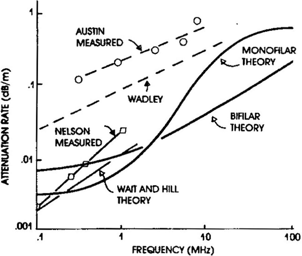
the frequency dependence and complexity of all the various modes of radio propagation underground are evident.23
Conclusions
The work undertaken on radio communication underground in South African mines in the 50 years after the issue was first raised in 1938, has been reviewed. Significant progress was made, particularly in the design of radio equipment suited to this demanding task. Modes of propagation, both directly through the rock and indirectly via any suitable conducting paths that spanned the area between transmitter and receiver, were identified and numerical data obtained to substantiate their characteristics.
Acknowledgements
I acknowledge the Chamber of Mines Research Organisation for some of the photographs and my erstwhile colleague, Graham Lambert, for taking the others.
Competing interests
I have no competing interests to declare.
Volume 120| Number 3/4 March/April 2024 25 https://doi.org/10.17159/sajs.2024/17301 Commentary Radio communications through rock strata Page 6 of 7
Figure 7: SC-100 portable transceiver used by a Rescue Training Station brigadesman wearing a full facemask.
Figure 8: The geology of the rock surrounding the test area underground devoid of all conductors.
Figure 9: Comparison between theoretical and measured attenuation rates with frequency for various modes of propagation underground.
references
1. Schonland BFJ. The work of the Bernard Price Institute of Geophysical Research, 1938-1951. Trans S Afr Inst Electr Eng. 1951;42(8):241–258.
2. Austin BA. Schonland: Scientist and soldier. London: IOPP; 2001. https://doi .org/10.1887/0750305010
3. Brain P. South African radar in World War II. Cape Town: SSS Radar Book Group; 1993.
4. Hewitt FJ. South Africa’s role in the development and use of radar in World War II. J Afr Mil Hist. 1975;3(3):88–93.
5. Vermeulen DJ. A history of electrical engineering in South Africa 1860-1960. Johannesburg: SAIEE; 2017.
6. Smith JR, Sturman B, Wright AF. The Tellurometer – from Dr Wadley to the MRA7. Cape Town: Tellumat; 2008.
7. Wadley TL. Radio communications through rock on the Witwatersrand mines. Telecommunications Research Laboratory, CSIR. August 1949, ETR-4.
8. Ames LA, Frazier JW, Orange AS. Geological and geophysical conditions in radio propagation through the earth’s crust. IEEE Trans Antennas Propag. 1963;AP-11:369–371. https://doi.org/10.1109/TAP.1963.1138027
9. Parkhomenko EI. Electrical properties of rocks. New York: Springer;1967. htt ps://doi.org/10.1007/978-1-4615-8609-8
10. Hansen RC. Radiation and reception with buried and submerged antennas. IEEE Trans Antennas Propag. 1963;AP-11:207–216. https://doi.org/10.110 9/TAP.1963.1138040
11. Wait JR. Electromagnetic fields of sources in lossy media. In: Collin RE, Zucker FJ, editors. Antenna theory: Part 2. New York: McGraw-Hill; 1969. p. 438–513.
12. Lang J. BullionJohannesburg: Men, mines and the challenge of conflict. Johannesburg: Jonathan Ball Publishers; 1986.
13. Vermeulen DJ, Blignaut P J. Underground radio communications and its application for use in mine emergencies. Trans S Afr Inst Electr Eng. 1961;52(4):94–109.
14. Wait JR. Electromagnetic waves in stratified media. IEEE; 1996.
15. Cory TS. Propagation of EM signals in underground mines, 1977. Final report Rockwell International for USBM, Contract No. H00366028.
16. Austin BA. Single-sideband transceiver design. Wireless World. 1978;84(1506):75–76.
17. Austin BA. Underground radio communication techniques and systems in South African mines. Proceedings of the Workshop on EM Guided Waves in Mine Environments; 1978 March 28–30; Boulder, CO, USA. p.87–102.
18. Hill DA, Wait JR. Excitation of monofilar and bifilar modes on a transmission line in a circular tunnel. J Appl Phys. 1974;45:3402–3406. https://doi.org/1 0.1063/1.1663792
19. Austin BA, Kerdic I. Transmission of radio signals in deep-level gold mines indirectly via power cables. Elec Letts. 1977;13(16):462–463. https://doi.or g/10.1049/el:19770333
20. Emslie AG, Lagace RL. Propagation of low and medium frequency radio waves in a coal seam. Radio Sci. 1976;11(4):253–261. https://doi.org/10 .1029/RS011i004p00253
21. Nelson TU. Propagation of MF signals along mine tunnel containing an axial wire and water trough. Elec Letts. 1980;16(22):834–836. https://doi.org/10 .1049/el:19800593
22. Wait JR, Hill DA. Radio frequency transmission via a trolley wire in a tunnel with a rail return. IEEE Trans Antennas Propag. 1977;AP-25(2): 248–253. htt ps://doi.org/10.1109/TAP.1977.1141558
23. Austin BA, Lambert GP. Electromagnetic propagation underground with special reference to mining. Trans SAIEE. 1985;76(1):1–5.
Volume 120| Number 3/4 March/April 2024 26 https://doi.org/10.17159/sajs.2024/17301 Commentary Radio communications through rock strata Page 7 of 7
AuthOR:
Mesias Alfeus1,2
AFFILIAtIONS:
1Department of Statistics and Actuarial Science, Faculty of Economics and Management Science, Stellenbosch University, Stellenbosch, South Africa
2National Institute for Theoretical and Computational Sciences, Stellenbosch, South Africa
CORRESPONDENCE tO:
Mesias Alfeus
EMAIL:
mesias@sun.ac.za
hOW tO CItE:
Alfeus M. Navigating the JIBAR transition: Progress, impacts, readiness, and analytical insights.
S Afr J Sci. 2024;120(3/4), Art. #17841. https://doi.org/10.17159/sa
js.2024/17841
ARtICLE INCLuDES:
☐ Peer review
☐ Supplementary material
KEYWORDS:
JIBAR transition, interest rate markets, derivative pricing, Monte Carlo method, Wishart process
FuNDING:
South African Department of Science and Innovation, NITheCS
Implementation of Industry Directed Research Programme (DSI/CON C3025, 2023)
PuBLIShED:
27 March 2024
Navigating the JIBAR transition: Progress, impacts, readiness, and analytical insights
Significance:
The move away from LIBOR to new risk-free rates is crucial in finance. In this Commentary, I examine South Africa’s readiness for transitioning from JIBAR to these new rates, especially regarding interest rate derivatives. I delve into how this shift impacts pricing, unique to South Africa’s market. Using a mathematical model based on a 2 × 2 Wishart process, I analyse caplet pricing considering backward- and forwardlooking rates. Comparing these caplet types reveals the complexities of pricing in this changing financial landscape. The insights shed light on challenges and opportunities for South Africa and the finance sector as JIBAR nears its end, emphasising the need for robust mathematical strategies in navigating this transition.
Introduction
The world of Quantitative Finance and Risk Management has changed significantly since the 2007–2008 Global Financial Crisis (GFC). Problems that used to have simple answers in finance have become more complicated. Quantitative analysts, often called quants, used to be very confident in their understanding of the basics of financial modelling. These basics included clear benchmarks like LIBOR and JIBAR, reliable interbank credit, and stable single currency values (as mentioned by others1,2).
The financial mathematics community found itself confronted with the task of pricing progressively intricate structured financial products. However, the landscape was irrevocably altered by the GFC, introducing uncertainties stemming from unreliable market interbank credit and the volatility in frequency basis. Consequently, the industry responded by introducing the multi-curve pricing framework – a paradigm that entails the construction of multiple yield curves, each tailored to a specific tenor.3
In the context of South Africa, the transition away from the Johannesburg Interbank Agreed Rate (JIBAR) has emerged as a significant financial endeavour. This Commentary undertakes an exploration of the progress achieved thus far, the ramifications for a relatively modest market, the readiness of South Africa to navigate the complexities of the JIBAR transition, and the indispensable analytical groundwork required to ensure a seamless and prosperous shift away from JIBAR.
LIBOR and JIBAR background
LIBOR
In the early 1980s, financial institutions initiated a quest for a standardised benchmark to facilitate the pricing of a diverse array of financial instruments. The London Interbank Offered Rate (LIBOR), which made its inaugural appearance in 1986, emerged as the predominant benchmark within this context. LIBOR is defined as the rate at which an individual Contributor Panel bank could borrow funds.
It is essential to underscore that the rate submitted by each bank must be derived from the institution’s assessment of its funding costs within the interbank market. In this context, “funds” encompasses unsecured interbank cash and funds procured through the primary issuance of interbank Certificates of Deposit.
However, in September 2012, Barclays Bank incurred a substantial fine of GBP290 million due to its illicit efforts to manipulate LIBOR. Such instances of benchmark rate manipulation, driven by individual and institutional interests, engendered diminished reliance on the benchmark and cast doubts upon its future viability. Consequently, the volume of transactions referencing LIBOR witnessed a noteworthy decline. In response, diverse working groups were convened to orchestrate international endeavours aimed at reviewing and reforming interest rate benchmarks. The overarching objective is to supplant existing benchmarks with risk-free or nearly risk-free rates.
The International Organization of Securities Commissions (IOSCO) has promulgated a set of guiding principles that pertain to benchmark rates. These principles encompass considerations of appropriateness, design, integrity, and efficacy. A pivotal aspect of these principles involves an assessment of the sufficiency of transaction volumes to serve as the foundation for a benchmark reference rate.
Within markets confronting the impending obsolescence of Interbank Offered Rates (IBORs), most notably those heavily reliant on LIBOR, a complex and protracted transition process becomes imperative.
JIBAR
JIBAR constitutes a prominent benchmark interest rate within the financial landscape of South Africa. Its functionality bears a resemblance to that of other IBORs, such as LIBOR, playing a pivotal role as a reference rate in diverse financial transactions, encompassing loans, derivatives, and various other financial instruments. JIBAR’s calculation process involves the collaboration of five contributing banks, namely Standard Bank, Nedbank, FirstRand Bank, Absa, and Investec. On a daily basis, these banks disseminate a series of money market rates, signifying their willingness to engage in the purchase and sale of Negotiable Certificates of Deposit (NCD) to entities including the Johannesburg Stock Exchange (JSE) and the South African Reserve Bank (SARB). Subsequently, the
27 https://doi.org/10.17159/sajs.2024/17841 Volume 120| Number 3/4 March/April 2024 © 2024. The Author(s). Published under a Creative Commons Attribution Licence. Commentary
benchmark administrator, SARB, calculates the average midpoints based on these NCD rates for varying tenors, specifically, one month, three months, six months, and twelve months. It is worth noting that the threemonth JIBAR rate holds particular significance within the South African financial landscape, serving as a critical reference rate for numerous loans, derivatives, and financial products.
Much akin to LIBOR, JIBAR carries inherent risks related to bank liquidity and interbank dynamics, potentially rendering it susceptible to substantial instability, especially during periods characterised by heightened volatility. Furthermore, its foundation rests upon an expert judgement model, thereby rendering it susceptible to potential attempts at manipulation. In light of these considerations, a strong impetus exists within the South African financial sector to mitigate the risks associated with rate manipulation, augment market integrity, and ensure that benchmark rates derive from genuine market transactions rather than expert judgements.
Practitioners active in South Africa’s interest rate markets have raised legitimate questions regarding the necessity of transitioning from JIBAR to an alternative risk-free rate. Notably, JIBAR fails to conform to the sufficiency guidelines delineated by the IOSCO, prompting the SARB to embarkonareformativetrajectoryakintothetransformationsundertaken by other central banks in relation to IBORs. During this transitional phase, an interim enhancement framework has been introduced, designed to fortify JIBAR over a finite period, pending the adoption of an alternative reference rate. A central facet of this enhancement revolves around elevating the obligation size imposed upon each contributing bank – a notable shift from the previous obligation of ZA100 million per point on the NCD curve to the current threshold of ZAR500 million per point. This augmentation serves to enhance JIBAR’s adherence to the sufficiency principle delineated by IOSCO, thereby bolstering its robustness.
Anticipations regarding the alternative reference rate posit its character as a risk-free or near-risk-free benchmark, potentially devoid of term structure. In this context, ZARONIA (South African Overnight Index Average), derived from the repo market, has been embraced as the alternative reference rate of choice, symbolising a steadfast commitment to heightened transparency and accuracy within the South African financial landscape.4 ZARONIA, renowned for its origins and reliability, emerges as a compelling candidate to supplant JIBAR, serving as a more representative indicator of short-term borrowing costs. Its robust attributes further accentuate its suitability for the role of JIBAR’s successor.
Table 1 provides a statistical snapshot of the JIBAR and ZARONIA rates over the specified period. The relatively low standard deviations, detrended values, and nonlinear detrended values suggest that the rates remained stable, with limited variations and trends. The positive spot spread indicates that JIBAR rates tended to be higher than ZARONIA rates during this period. The values for detrended standard deviation are relatively low for both JIBAR and ZARONIA, indicating that, even after removing trends, the rates remained relatively stable. Negative values for kurtosis and skewness for both JIBAR and ZARONIA suggest
table 1: Descriptive statistics of South African benchmark rates
-month JIBAR and ZARONIA), 28 July 2022 to 19 September 2023
Mean 7.39807.01580.3821
Standard deviation (s.d.)0.92140.93380.0760
Detrended s.d.0.24140.22040.0738
Nonlinear detrended s.d.0.15960.17230.0594
Kurtosis -1.0076-1.06670.4772
Skewness -0.4552-0.38580.2495
Data source: South African Reserve Bank5
that the rate distributions are leptokurtic and negatively skewed. This means that the rate distributions have thinner tails and are skewed to the left (negatively). Figure 1 provides a time-series representation of the relationship between JIBAR and ZARONIA over the course of approximately 14 months (data were collected from the South African Reserve Bank website from 28 July 2022 to 19 September 2023). It suggests a positive correlation between JIBAR and ZARONIA.
South Africa’s readiness
A crucial question arises about how prepared South Africa is for the upcoming change. In my view, rushing this transition might not be necessary. South Africa’s financial world is quite small, mainly involving five important banks that play a big role in determining the JIBAR. Unlike bigger and more developed financial markets, the risk of manipulating JIBAR in South Africa is much lower.
Therefore, there is no need to hurry with this transition to risk-free rates. We should remember that JIBAR will eventually not be used, but we do not know when exactly that will be. JIBAR is based on banks lending to each other without any guarantees, while the new benchmark rates are based on safer transactions without credit factors. Switching to these safer transactions raises important questions about how it will affect financial markets.
The SARB has taken proactive steps by creating a special group to find a new, suitable risk-free rate, similar to what was done in the USA and UK when they moved away from IBOR. Globally, there is a preference for using a very safe rate. However, it is crucial to recognise that many financial markets do not meet the requirements to develop such rates. Therefore, many markets, like the European Union and Japan, have chosen to quickly adopt nearly risk-free overnight and secured rates.
The SARB has made it clear that they want to approach this transition carefully to avoid causing instability and market swings. They are committed to following the best international practices.
Additionally, the uncertainty about JIBAR’s future has raised questions about its current impact on swaps and agreements. The shift to new reference rates may affect derivative hedging. One major concern is not knowing if there will be a way to hedge existing loans and debt linked to the 3-month JIBAR after the transition. This situation could lead to a risk of differences between privately agreed loans and their related derivatives. Moreover, introducing new benchmark rates could significantly change the way existing hedging strategies work.
Derivative pricing
I initiate the discussion by exploring derivative pricing, specifically in the context of employing an alternative risk-free rate. In this regard, I examine the effective daily compounding rate applied retrospectively over the time interval Tj 1, Tj:
ARR(Tj 1, Tj) := 1 τj (∏ i=1 N (1 + δi RF Ri(ti)) 1), ∀i, ti ∈ [T 1, T ], Equation 1
where RF Ri(t) for i ∈ 1, ,N denotes the alternative overnight rates in the given reference period. In Equation 1, the variable τj signifies the cash day count fraction relevant to the accrued period, while δ pertains to the cash day count fraction corresponding to the overnight accrued period. Importantly, this rate encapsulates the actual rate operative over the specified period, distinguishing itself by its reduced volatility when contrasted with an average rate. It derives its foundation from the wellestablished Overnight Index Swap market, leveraging the extant crosshedging capabilities inherent within this market.
Overnight risk-free rates distinguish themselves by their inherent riskfree or nearly risk-free nature, in stark contrast to the IBORs which encompass an amalgamation of factors, including a bank credit risk premium, liquidity considerations, and supply–demand dynamics. In the event of the permanent discontinuation of the pertinent IBORs,
Volume 120| Number 3/4 March/April 2024 28 https://doi.org/10.17159/sajs.2024/17841 Commentary Navigating the JIBAR transition Page 2 of 6
spread (%)
JIBAR (%)ZARONIA (%)Spot
(3
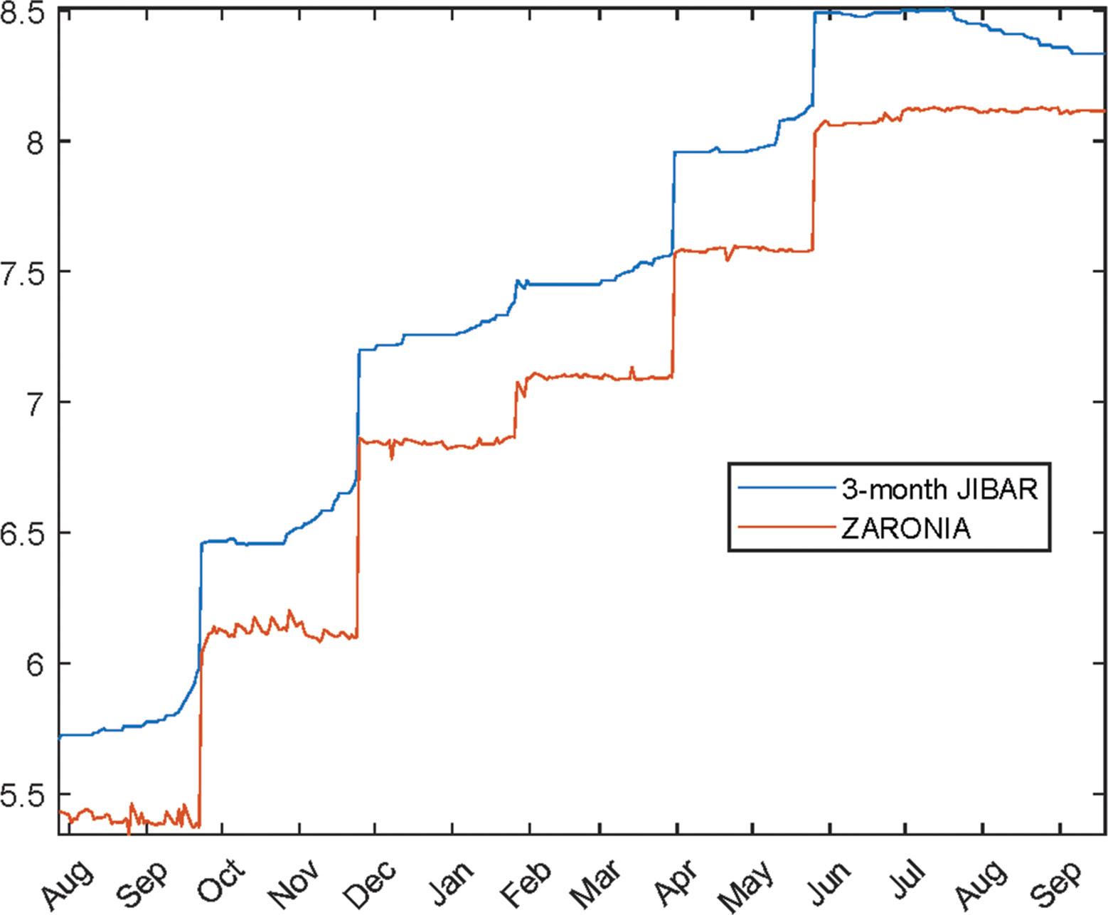
Data source: South African Reserve Bank5
it becomes impractical to entirely replicate these multifaceted determinants. However, a judicious approach entails the application of a spread adjustment to the corresponding adjusted risk-free rates. The methodologies underlying this approach are devised with three primary objectives in mind:
•To effectuate the elimination or minimisation of value transfer ramifications at the juncture when the fallback is instituted.
•To eradicate or mitigate any potential for manipulation, thereby safeguarding the integrity of the transition process.
•To eliminate or mitigate against the disruptive impact on financial markets that may ensue at the moment that the fallback mechanism is activated.
Spread adjustment
As outlined in the current ISDA protocol6, the primary alternative for derivatives linked to LIBOR rates involves using the combined overnight risk-free rate along with an extra credit adjustment spread.
The spread adjustment could be calculated based on observed market prices for the forward spread between the relevant IBOR and the adjusted risk-free rates in the relevant tenor at the time when the fallback is triggered. The spread is given by:
S(t) = FL(t) FR(t),
Equation 2
where FL is the t forward LIBOR rate and FR is the t forward risk-free rate. This spread gives a current representation of the prevailing market conditions and forward expectations. The fallback rate is then given by:
F(t) = FR(t) + S(t)
Equation 3
19 September 2023.
Wishart processes
The application of Wishart processes in finance is central as it incorporates risks characterised by volatility-covolatility matrices. To acquaint oneself with the foundational concepts related to Wishart processes, it is recommended to refer to seminal works7-9 and the contributions of Gnoatto and collaborators10,11. Additionally, the PhD thesis by Gnoatto12 provides comprehensive insights into this subject.
Let us begin with a formal definition:
Definition 1. Consider a d × d-dimensional Brownian motion W (W ∼ ℬℳd), along with arbitrary matrices Q and M belonging to ℳd(ℝ), an initial value x0 within the closure of positive semidefinite real d × d matrices (x0 ∈ ��d +), and a non-negative parameter α. The Wishart stochastic differential equation is represented as:
d Xt = (Xt M + M′ Xt + αQ′Q)dt + √Xt d Wt Q + Q′d Wt ′ √Xt , ; X0 = x0
Equation 4
Here, X is a strong solution within ��d +, characterising a Wishart process with parameters Q, M, α, and x0. This process is conventionally denoted as X ∼ ����d(Q, M, α, x0)
In the modelling context, define the filtered probability space (Ω, ℱ, (ℱ��)t≥0 , ℚ) and assume that the short rate is driven by a Wishart process X, specifically:
RFR(t) = λ0 + tr[Λ Xt] for all t ≥ 0.
Equation 5
Here, Λ belongs to ��d +, and λ0 is a scalar. It is essential to note that tr[ ] signifies the trace operator applicable to any square matrix.
Volume 120| Number 3/4 March/April 2024 29 https://doi.org/10.17159/sajs.2024/17841 Commentary Navigating the JIBAR transition Page 3 of 6
Figure 1: Analysing the dynamic interplay: JIBAR and ZARONIA rates, 28 July 2022 to
Monte Carlo pricing
In the domain of quantitative finance, the pricing of intricate financial derivatives frequently demands the application of advanced mathematical models and computational methodologies. One such derivative is the caplet, a financial contract that grants the holder the privilege to receive payments if a reference interest rate surpasses a predetermined strike rate. In this illustrative instance, I embark on the evaluation of caplet pricing, employing a Monte Carlo simulation approach (for a comprehensive discussion of this method, please refer to Glasserman13). What adds a noteworthy dimension to this scenario is the contemplation of both backward-looking and forward-looking caplets (each follows a 2 × 2 Wishart process). These processes are characterised by specific parameters, including volatility and drift matrices, providing valuable insights into the complexities of modelling interest rate dynamics, and valuing these derivative instruments.
The payoff of the caplet over the period [T 1, T ] is given by:
τ ( 1 τj (∏ i 1 N (1 + δi RF Ri(ti)) 1) + S(t) K)+
Equation 7
Equation 7 can be straightforwardly evaluated through numerical methods, such as Monte Carlo simulation. In this approach, we assume that the underlying alternative risk-free rate adheres to the Wishart process outlined in Equation 4. In the subsequent experiment, we specifically examine the following instance of the Wishart process:
Equation 6
where K is the strike price of the caplet. This is equivalent to a geometric Asian option. The price at time t ≤ Tj 1 of this option is computed as:
Table 2 and Figure 2 depict the pricing distinctions between forwardand backward-looking caplets in the context of a Wishart process. As observed, as documented in previous research14, forward-looking caplets consistently exhibit lower valuations in comparison to their backward-looking counterparts. This disparity underscores the significance of comprehending the distinctive characteristics of these Strike0.0250.030.0350.040.0450.050.0550.060.065
small,
a
Backward caplet
Forward caplet
slightly higher values than forward
in the
Price0.04300.04060.03820.03590.03350.03120.02880.02650.0241
s.e.2.840e-052.8314e-052.8234e-052.8404e-052.8953e-052.870e-052.8820e-052.9052e-052.9058e-05
Price0.04230.04000.03760.03530.03290.03050.02830.02570.0235
s.e.4.723e-054.7860e-054.8295e-054.8157e-054.8140e-054.8502e-054.8525e-054.8265e-054.8746e-05
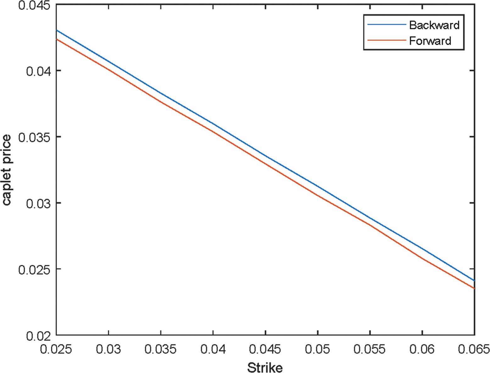
Volume 120| Number 3/4 March/April 2024 30 https://doi.org/10.17159/sajs.2024/17841 Commentary Navigating the JIBAR transition Page 4 of 6
ct = ��t ℚ[e ∫ T RFR(s)ds τj ( 1 τj (∏ i=1 N (1 + δi RF Ri(ti)) 1) + S(t) K)+]
M = (0.030.02 0.020.035), Q = ( 0.020.015 0.015 0.025), X0 = ( 0.040.045 0.045 0.05 ), A = (1.00 0.00 0.00 1.00), α = 0.1
table 2: Monte Carlo prices and standard errors (s.e.) for backward and forward caplets, with backward caplets showing
caplets. Additionally, the Monte Carlo standard errors for these prices are exceptionally
indicating
high level of precision
simulation results. The spread adjustment S = 0.003821.
Figure 2: Comparison of caplet prices: forward vs backward looking rates in a Wishart process.
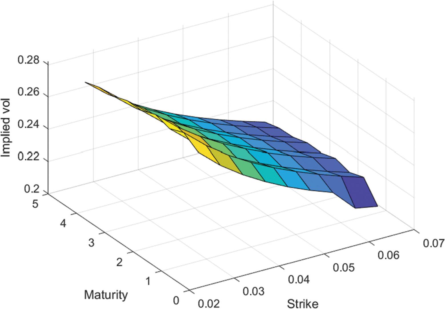
caplets in the realm of risk management and financial decision-making, especially in the context of emerging benchmark risk-free rates.
Figure 3 presents the volatility surface of backward-looking caplets, computed using a Fourier-based method as discussed by Fantana14 , within the framework of a Wishart process. This visualisation offers valuable insights into the complex dynamics of interest rate derivatives.
Conclusion
As highlighted by SARB4, the process of transitioning from JIBAR to alternative reference rates in South Africa represents a substantial and pivotal endeavour, bearing significant implications for the nation’s financial markets. Notable advancements have been achieved in this endeavour, encompassing the establishment of an alternative reference rate, ZARONIA, and the extensive dissemination of knowledge within the market. Nonetheless, the transition is accompanied by persistent challenges, particularly in the context of adapting to the distinctive characteristics inherent to South Africa’s financial landscape.
The consequences of this transition, particularly within a relatively compact market, underscore the importance of meticulous analysis and effective risk management. The indication of South Africa’s readiness, propelled by regulatory backing and proactive involvement of market participants, is a positive signal. However, it is imperative to maintain a vigilant stance, ensure clear communication, and undertake comprehensive analyses as the transition unfolds. By actively addressing the identified challenges and conducting the requisite analyses, South Africa can navigate the JIBAR transition with success, ultimately contributing to the cultivation of a more resilient and transparent financial system for the foreseeable future (see for example Backwell et al.15).
Acknowledgements
I thank the Editor-in-Chief Prof. Leslie Swartz, two anonymous readers, and Prof. Justin Harvey. I acknowledge financial support from the Department of Science and Innovation (DSI) and the NITheCS Implementation of Industry Directed Research Programme (IDRP) [DSI/ CON C3025, 2023].
Competing interests
I have no competing interests to declare.
References
1. Frishling V. Transition to new benchmark – abandoning LIBOR. Melbourne: National Australia Bank; 2019.
2. Lyashenko A, Mercurio F. Looking forward to backward-looking rates: A modeling framework for term rates replacing LIBOR. SSRN. 6 February 2019. https://doi.org/10.2139/ssrn.3330240
3. Alfeus M, Grasselli M, Schlögl E. A consistent stochastic model of the term structure of interest rates for multiple tenors. J Econ Dyn Control. 2020;114, Art. #103861. https://doi.org/10.1016/j.jedc.2020.103861
4. South African Reserve Bank (SARB). Draft statement of methodology and the policies governing the South African Reserve Bank-administered interest rate benchmarks. Pretoria: SARB; 2020.
5. South African Reserve Bank (SARB). ZARONIA interest rate benchmark [webpage on the Internet]. No date [cited 2023 Sep 20]. Available from: https://www.resbank.co.za/en/home/what-we-do/financial-markets/ south-african-overnight-index-average
6. ISDA. IBOR Fallbacks Protocol. ISDA; 2020. Available from: https://www.i sda.org
7. Bru M. Wishart processes. J Theor Probab. 1991;4(4):725–751. https://doi.org /10.1007/BF01259552
8. Gourieroux C. Continuous time Wishart process for stochastic risk. Econ Rev. 2006;25(2):117–217. https://doi.org/10.1080/07474930600713234
9. Baldeaux J, Platen E. Functionals of multidimensional diffusions with applications to finance. Cham: Springer; 2013. https://doi.org/10.1007/97 8-3-319-00747-2
10. Gnoatto A, Grasselli M, Fonseca JD. A flexible matrix Libor model with smiles. J Econ Dyn Control. 2013;37(4):774–793. https://doi.org/10.1016/j.jedc.201 2.11.006
11. Gnoatto A, Grasselli M. The explicit Laplace transform for the Wishart process. J Appl Probab. 2014;51(3):640–656. https://doi.org/10.1239/jap /1409932664
Volume 120| Number 3/4 March/April 2024 31 https://doi.org/10.17159/sajs.2024/17841 Commentary Navigating the JIBAR transition Page 5 of 6
Figure 3: Volatility surface of backward-looking caplets computed using the Fourier-based method in a Wishart process.
12. Gnoatto A. Wishart processes: Theory and applications in mathematical finance [PhD thesis]. Padua: University of Padua; 2012.
13. Glasserman P. Monte Carlo methods in financial engineering. New York: Springer-Verlag; 2003. https://doi.org/10.1007/978-0-387-21617-1
Navigating the JIBAR transition
14. Fantana C. Short Communication: Caplet pricing in affine models for alternative risk-free rates. Siam J Financial Math. 2023;14(1):sc1–sc16. http s://doi.org/10.1137/22M1513691
15. Backwell A, Macrina A, Schlögl E, Skovmand D. Lost in the Libor transition [preprint]. SSRN; 19 September 2023. https://dx.doi.org/10.2139/ssrn.4575993
Volume 120| Number 3/4 March/April 2024 32
Commentary
https://doi.org/10.17159/sajs.2024/17841
Page
of 6
6
AuThor: Douglas A. Parry1
AFFILIATIoN:
1Department of Information Science, Stellenbosch University, Stellenbosch, South Africa
CorrESPoNDENCE To: Douglas Parry
EMAIL:
dougaparry@sun.ac.za
hoW To CITE:
Parry DA. Without access to social media platform data, we risk being left in the dark. S Afr J Sci. 2024;120(3/4), Art. #17008. https:// doi.org/10.17159/sajs.2024/17008
ArTICLE INCLuDES:
☐ Peer review
☐ Supplementary material
KEYWorDS:
social media data, digital trace data, data access, Digital Services Act, DSA
PubLIShED: 27 March 2024
Without access to social media platform data, we risk being left in the dark
Significance:
Social media data are essential for studying human behaviour and understanding potential systemic risks. Social media platforms have, however, begun to remove access to these data. In response, other countries and regions have implemented legislation that compels platforms to provide researchers with data access. In South Africa, we have lagged behind the Global North when it comes to using platform data in our research and, given the recent access restrictions, we risk being left behind. In this Commentary, I call attention to this critical issue and initiate a conversation about access to social media data in South Africa.
Subatomic particle physics has CERN. Astronomy has the Hubble telescope. Social science has the Internet, smartphones, email, social media, satellites, and a myriad of other ways to follow human behavior. The gods of the information age have produced a whole panoply of technologies for social research along the journey to other destinations.
–David Lazer1
For scientists interested in understanding the character and effects of individual and collective behaviour, the digital age has brought about new opportunities to observe and measure human interaction at scale.2 The Internet, and social media platforms in particular, provides us with unprecedented (albeit socially and algorithmically biased)2,3 access to robust data on these interactions4. Facebook, Instagram, Twitter/X, TikTok and other social media platforms have not only fundamentally altered the ways in which we communicate with others but, by scaffolding how we interact with and engage with individuals, ideas, and organisations, they have reconfigured the public sphere itself. Throughout our everyday use of these platforms, we leave behind digital traces of our behaviour as by-products of our interactions with other users and entities.5 These digital traces hold tremendous value for studying the nature and consequences of (mediated) human behaviour at individual, group, and population levels. For example, through social media platform data we can investigate, among other things, misinformation campaigns, election interference, the spread of infectious diseases, polarisation, and the effects of particular interaction patterns on user’s mental health and well-being.6-8 Collectively, such data provide an important lens that enables both fundamental research on human behaviour as well as research on the potential systemic societal and economic risks posed by social media platforms. This importance is reflected in the growing prominence of computational social science across academic disciplines.9
Despite the considerable opportunities that these data hold, and the widespread use of computational social science in the Global North, research in South Africa, and the Global South more generally, has thus far made only limited use of digital trace data compared to the engagement observed in the Global North.10,11 While there are likely many factors underlying this general disparity, and numerous counter examples of interesting studies in the Global South leveraging digital trace data, unpacking these factors falls outside the scope of this comment. For now, it is sufficient to acknowledge the existence of this general disparity. Despite only limited use of digital trace data collected from social media platforms in South Africa, it is no less important here than it is in the Global North that we understand how these platforms impact, for better or worse, ordinary South Africans, our society at large, and potentially our hard-fought democracy.
“The way is shut” – restrictions on access to social media data
Unfortunately, while social media platforms continue to collect and analyse user data, in the wake of various scandals, the fears surrounding unfettered data use for the training of large-language models, and a general reluctance to face external scrutiny, most social media platforms have restricted and/or entirely removed access to the application programming interfaces (APIs) that researchers used to access platform data.12-14 The shuttering of these APIs has brought large swathes of social media research to a halt and, in doing so, severely jeopardised the extent to which we can learn about behaviour online and the very real consequences that this behaviour can have for individuals and societies.12,15
While alternative approaches to collecting social media data exist (e.g. self-reports, web scraping, browser extensions, data donations)5, and some researchers have partnered directly with social media platforms to access data, for various reasons these techniques fall short of the high-quality individual-level data available directly from platforms4,5,14, or in the case of direct partnerships, are only available to a select privileged few (who are almost exclusively based at institutions in the Global North). For this reason, we require direct, equitable access to social media data, without which we will be left in the dark when it comes to important individual and societal questions.
“A light from the shadows shall spring” – regulations to compel data access
In response to these restrictions and the broader recognition of the power that online platforms hold, the European Commission has implemented several key regulations as part of a broader set of legislation designed to govern the digital sphere in the European Union (EU). With the aim of fostering a safer online environment, the Digital Services Act (DSA) will, among other things, compel online platforms operating within the EU to prevent and remove posts containing illegal content, to ban certain types of targeted advertising (e.g. sexual orientation, religion), and to provide greater transparency into how their content algorithms work. For “very large online platforms” (i.e. those
33 https://doi.org/10.17159/sajs.2024/17008 Volume 120| Number 3/4 March/April 2024 © 2024. The Author(s). Published under a Creative Commons Attribution Licence. Commentary
with at least 45 million monthly users in the EU, which covers most popular social media platforms and many other more general services like Booking.com and Google Maps), the act also requires that platforms (1) enable users to be able to opt out of recommendation systems, (2) be subject to external and independent audits, and (3) share data with researchers and other vetted independent ‘watchdog’ organisations.
This latter requirement, described in Article 40 of the DSA (see https ://www.eu-digital-services-act.com/Digital_Services_Act_Article_40. html for the full text), is particularly important given the stranglehold that platforms have over access to data. Article 40 of the DSA compels very large online platforms to provide vetted researchers with access to data “for the sole purpose of conducting research that contributes to the detection, identification and understanding of systemic risks in the Union” and sets out the rules governing this access. While the DSA has been in effect since 25 August 2023, the code of conduct for practical compliance with the regulations remains a work in progress, and the full implementation will occur only in 2024 (see Klinger and Ohme16 for a set of recommendations for what this should look like). Indeed, managing vetted researcher access to platform data poses substantial challenges for the protection of personal user data and privacy, but also for the design, implementation, and running of the necessary infrastructure to securely manage, store, and process researcher data access. Despite these challenges, the DSA, and Article 40 in particular, provides an important example for other countries seeking to break the stranglehold that social media platforms have over their data, and enable robust and equitable access to critical data for research purposes.
Although research using digital trace data collected from social media platforms in South Africa has lagged behind research conducted in the Global North, given the rapidly growing adoption of mobile Internetconnected communications technologies (i.e. smartphones), the increasing roll-out of 5G bandwidth, and the general digitalisation of our economy, it is likely that there exists a similar potential for systemic societal risks posed by social media platforms here as there is in other countries. Unfortunately, given the ongoing restrictions and closing of platform APIs, South African researchers are left without any reliable, legal means of accessing data from social media platforms. Without access to social media data, not only do we risk getting left behind when it comes to research on important topics (e.g. misinformation, online political interference, digital well-being) but, perhaps more importantly, we are left without any means of developing insight at scale into online behaviour and the potential risks that it imposes for South Africans and South African society.
“All we have to decide is what to do with the time that is given to us” – an example of how to move forward
To ensure free and objective research on behaviour on social media platforms and the potential systemic risks that actions on these platforms can pose for individuals and society, we require reliable access to platform data. The EU has set an example for how this access can be achieved. While it would be naïve to assume that South Africa holds the same degree of economic clout to impose similar regulations on platforms with any chance of them being effective, we should not be afraid to explore other creative possibilities to enable research with digital trace data to flourish and contribute to our collective understanding of the character and risks of online behaviour. These possibilities could include the development of infrastructure for data donation at scale or the establishment of large-scale consortia to leverage current best practices to collect and integrate available data (see, for example, the European Digital Media Observatory project). Alongside these possibilities, I propose that we embrace the ‘Brussels effect’ (i.e. the de facto though not necessarily de jure externalising of EU regulations outside of the region’s borders due to various market mechanisms) and seek to leverage the DSA by (1) lobbying the South African government to implement similar regulations ‘piggybacking’ on the DSA, (2) coordinating with relevant stakeholders in the EU to ensure that the
code of conduct makes provision for broader access (see Klinger and Ohme16), and (3) in lieu of formal policy, collaborating with researchers in the EU who will have access to social media platform data.
My second and third propositions extend from the fact that the DSA is implemented on the basis of the ‘market location principle’ (lex loci solutionis), which holds that, irrespective of the location at which the platform was established, because the platform offers services in the EU/to EU citizens, non-European data also fall within the scope of the regulations. This implies that data from South African social media users will be available to researchers within the EU (but not presently researchers in South Africa). Notably, Article 40 does not necessarily preclude access to individuals based outside of the EU. Article 40(8)(a) of the DSA read together with Article 2, point 1 of the Digital Single Market Directive suggests that to be eligible to access platform data one should be affiliated with a non-profit entity located in any country devoted to scientific research. The regulation does, however, restrict the geographic scope of the research foci for which access to platform data will be provided. Both Article 40(4) and Article 40(12) suggest that the research must study “systemic risks in the Union.” In a broad interpretation of this restriction, Husovec17 argues that “research focusing on risks in the Union needs to study non-EU countries to be scientifically sound.” This interpretation suggests that, notwithstanding the data privacy concerns associated with cross-border data sharing and the practicalities of data access outside the EU, with careful justification, we can leverage this legislation to access data on South African social media users. Regardless, our ‘first prize’ would be the production of similar legislation in South Africa (proposition 1) so that we can avoid being reliant on partnerships with researchers in the EU. In doing so, we would not be alone; recognising the growing prominence of the digital/online environment, many other countries are developing legislation in this regard. The UK Online Safety Bill, for example, contains similar provisions to the DSA.
With this Commentary I have aimed to call attention to this critical issue, highlight the need for increased use of digital trace data in South African research, raise concerns about our rapidly disappearing access to platform data, and initiate a conversation about the need for policy enabling research with social media data in South Africa. While the EU has provided an example for how we can achieve increased transparency and access to social media data, developing and implementing the relevant legislation fit for our economy will not be an easy task. We will require input from experts in many disciplines (e.g. law, economics, computer science, and the social sciences at large) and the establishment of resource-intensive data intermediaries who can steward (collect, maintain, share) access to platform data as well as the development of infrastructure to enable and manage these procedures (data clean rooms, virtual laboratory environments, etc.), all while being mindful of the substantial ethical and privacy risks posed by increased data access (see de Vreese and Tromble14 for a discussion of how research data access can co-exist with data privacy regulations, and point five in Klinger and Ohme16 for recommendations on how data sensitivity can be managed). Despite these challenges, I believe that, without proactive effort, we risk being left behind without any robust means of studying the potential systemic risks at play.
Competing interests
I have no competing interests to declare.
references
1. Lazer D. Social science, today. Science. 2018;359(6371):42. https://doi.org/10 .1126/science.aaq0679
2. LazerD,HargittaiE,FreelonD,Gonzalez-BailonS,MungerK,OgnyanovaK,etal. Meaningful measures of human society in the twenty-first century. Nature. 2021;595(7866):189–196. https://doi.org/10.1038/s41586-021-03660-7
3. Wagner C, Strohmaier M, Olteanu A, Kıcıman E, Contractor N, Eliassi-Rad T. Measuring algorithmically infused societies. Nature. 2021;595(7866), Art. #7866. https://doi.org/10.1038/s41586-021-03666-1
Volume 120| Number 3/4 March/April 2024 34 https://doi.org/10.17159/sajs.2024/17008 Commentary Access to social media platform data Page 2 of 3
4. Parry D, Davidson BI, Sewall CJR, Fisher JT, Mieczkowski H, Quintana DS. A systematic review and meta-analysis of discrepancies between logged and self-reported digital media use. Nat Hum Behav. 2021;5:1535–1547. https:// doi.org/10.1038/s41562-021-01117-5
5. Ohme J, Araujo T, Boeschoten L, Freelon D, Ram N, Reeves BB, et al. Digital trace data collection for social media effects research: APIs, data donation, and (screen) tracking. Commun Methods Meas. Forthcoming 2023. https://d oi.org/10.1080/19312458.2023.2181319
6. Guess AM, Malhotra N, Pan J, Barberá P, Allcott H, Brown T, et al. How do social media feed algorithms affect attitudes and behavior in an election campaign? Science. 2023;381(6656):398–404. https://doi.org/10.1126/sc ience.abp9364
7. Ruths D, Pfeffer J. Social media for large studies of behavior. Science. 2014;346(6213):1063–1064. https://doi.org/10.1126/science.346.6213.1063
8. Van Bavel JJ, Rathje S, Harris E, Robertson C, Sternisko A. How social media shapes polarization. Trends Cogn Sci. 2021;25(11):913–916. https://doi.org /10.1016/j.tics.2021.07.013
9. Lazer DMJ, Pentland A, Watts DJ, Aral S, Athey S, Contractor N, et al. Computational social science: Obstacles and opportunities. Science. 2020; 369(6507):1060–1062. https://doi.org/10.1126/science.aaz8170
10. Becerra G, Ratovicius C. Social sciences and humanities on big data: A bibliometric analysis. J Syst Inf Technol Man. 2022;19. https://doi.org/10. 4301/S1807-1775202219011
11. Ghai S, Fassi L, Awadh F, Orben A. Lack of sample diversity in research on adolescent depression and social media use: A scoping review and metaanalysis. Clin Psychol Sci. 2023;11(5):759–772. https://doi.org/10.1177/2 1677026221114859
12. Freelon D. Computational research in the post-API age. Polit Commun. 2018;35(4):665–668. https://doi.org/10.1080/10584609.2018.1477506
13. Davidson BI, Wischerath D, Racek D, Parry DA, Godwin E, Hinds J, et al. Platform-controlled social media APIs threaten open science. Nat Hum Behav. 2023;7(12):2054–2057. https://doi.org/10.1038/s41562-023-01750-2
14. De Vreese C, Tromble R. The data abyss: How lack of data access leaves research and society in the dark. Polit Commun. 2023;40(3):356–360. https ://doi.org/10.1080/10584609.2023.2207488
15. Bruns A. After the ‘APIcalypse’: Social media platforms and their fight against critical scholarly research. Inf Commun Soc. 2019;22(11):1544–1566. https ://doi.org/10.1080/1369118X.2019.1637447
16. Klinger U, Ohme J. What the scientific community needs from data access under Art. 40 DSA: 20 Points on infrastructures, participation, transparency, and funding. Weizenbaum Policy Paper 8. Berlin: Weizenbaum Institute for the Networked Society – The German Internet Institute; 2023. https://doi.org /10.34669/WI.WPP/8.2
17. Husovec M. How to facilitate data access under the Digital Services Act. SSRN; 2023 May 19. Available from: https://ssrn.com/abstract=4452940
Volume 120| Number 3/4 March/April 2024 35 https://doi.org/10.17159/sajs.2024/17008 Commentary Access to social media platform data Page 3 of 3
AuthorS:
Jonathan Jansen1
Cyrill Walters1*
Alistair White2
Graeme Mehl3
*Author deceased: 28 December 2023
AFFILIAtIoNS:
1Education Policy Studies, Stellenbosch University, Stellenbosch, South Africa
2National Research Foundation, Pretoria, South Africa
3Centre for Research on Evaluation, Science and Technology (CREST), Stellenbosch University, Stellenbosch, South Africa
CorrESPoNDENCE to:
Jonathan Jansen
EMAIL:
jonathanjansen@sun.ac.za
DAtES:
received: 18 Sep. 2023
revised: 22 Jan. 2024
Accepted: 26 Jan. 2024
Published: 27 Mar. 2024
hoW to CItE:
Jansen J, Walters C, White A, Mehl G. Why so few Ps become As: The character, choices and challenges of South Africa’s most talented young researchers. S Afr J Sci. 2024;120(3/4), Art. #16882. https:// doi.org/10.17159/sajs.2024/16882
ArtICLE INCLuDES:
☒ Peer review
☐ Supplementary material
DAtA AVAILABILItY:
☐ Open data set
☐ All data included
☒ On request from author(s)
☐ Not available
☐ Not applicable
EDItorS:
Chrissie Boughey
Nkosinathi Madondo
KEYWorDS:
networks, strategy, work ethic, motivation, transformation
FuNDING:
None
Why
so few
Ps become As: The character, choices and challenges of South Africa’s most talented young researchers
In this research article, we examine why so few of the most promising young scientists in South Africa, those who obtain a P or ‘prestigious’ rating from the South African National Research Foundation, go on to obtain an A rating, i.e. become leading international scholars in their fields. Drawing on in-depth interviews with 36 P-rated scientists in the period 1983 to 2022, we found that personal characteristics (such as work ethic), the right international networks, and strong departmental support are among the key factors that explain the research accomplishments of highly successful achievers.
Significance:
The research is significant for two reasons. It explains why so few promising young scientists in South Africa become world leaders in their respective fields and, in particular, why even fewer young black scientists achieve the highest ratings in their disciplines.
Introduction
In a companion study on young scientists (including social sciences and humanities scholars) with a rating from the South African National Research Foundation (NRF), we found that the P rating showed a poor predictive validity with respect to its granting assumption: that Ps were likely to become world leaders in their respective fields which, in NRF terms, means an A-rated scientist.1 In fact, of the 136 Ps awarded since inception (1983 to 2022), only 20 (14.7%) became As. Of these Ps, 21 were still in their P cycle in 2022. If we exclude them from the total, then 20 of 115 eligible Ps became As (17.4%). Figure 1 illustrates the progression of Ps to higher ratings between 1983 and 2022.
This does not mean that the P is not a good differentiator in terms of future success when compared with the lower rating for young scientists, that is, those who obtain the Y rating, as Figure 2 shows.
In this regard, two distinct trends emerge for P- and Y-rated researchers. For P-rated researchers, the distribution is skewed towards the higher rating categories, peaking at B1 (31%). In total, 78% of P-rated researchers (excluding those without further ratings) ended up achieving a rating of B2 or higher, while only 13% received a C rating (C1–C3).
For Y-rated researchers, the distribution is skewed towards the lower rating categories, peaking at C2. In total, 77% of Y-rated researchers (excluding those without further ratings) went on to receive a C rating (C1–C3), while only 24% went on to receive a rating of B3 or higher. It should be said that obtaining a P rating as a young scientist is an impressive achievement in its own right – not many P ratings are awarded by the NRF, and most young applicants who are rated would begin their careers with a Y rating.
Background
The NRF is a statutory body mandated by government to fund and support research and development in South Africa. One of its core functions is to assess and rate the scholarship of individual scientists through a peer-reviewbased rating system. Younger scientists, under the age of 35, can achieve a Y (Y1 or Y2) rating or the rare P rating. More established scientists compete to be awarded a C (C3, C2, C1) or B (B3, B2, B1) or A (A1, A2) rating with the stated gradations (in brackets) for each of them.
Each category of award has its own careful description. The Y is a promising young researcher, while the P is a prestigious award. The C is awarded to an established researcher, the B to an internationally acclaimed researcher, and the A to a leading international researcher. Each gradation within a category has an even more refined description to distinguish, say, a C3 from a much higher rating, the C1.
In the NRF stipulations, P awardees are those young scientists “considered likely to become future international leaders in their field” and who, in the review process, are “recognised by all or the overwhelming majority of reviewers as having demonstrated the potential of becoming future international leaders in their field on the basis of exceptional research performance and output”.
Given these heightened expectations, we wanted to know who exactly the Ps are and why so few of them became A-rated scientists.
Approach
This report represents qualitative research grounded in the etic or insider perspective on doing advanced research within universities. An initial interview protocol was piloted with non-participating young scientists and amended accordingly. The thick data generated from the 36 transcribed interview sets was qualitatively analysed for convergent and divergent themes, out of which emerged the seven key findings. This is a non-judgemental inquiry in that the words of the P-rated scientists represent their own experiences, methods, and ambitions.
36 https://doi.org/10.17159/sajs.2024/16882 Volume 120| Number 3/4 March/April 2024 © 2024. The Author(s). Published under a Creative Commons Attribution Licence. Research
Article
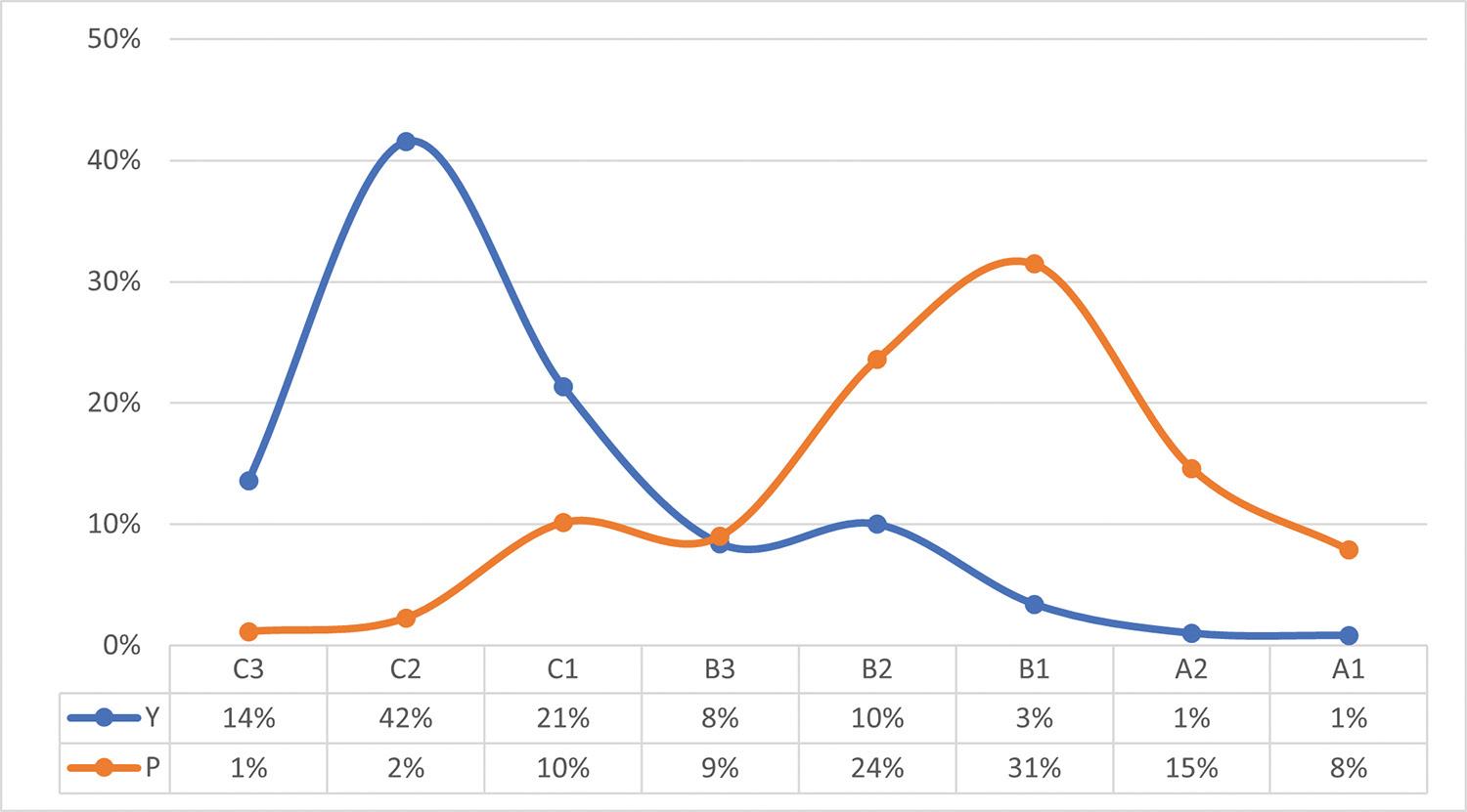
The themes induced deductively from the qualitative interviews are not mutually exclusive. Nor do we claim that they represent the full range of explanations for success or otherwise of young scientists striving to become top-rated senior researchers.
To understand the low conversion rate of Ps to As, we interviewed 36 of the 136 Ps (26.5%) who were sampled based on their availability, their disciplinary diversity, and the extent to which they enabled a more or less equal distribution of numbers in each of the following three categories:
• In category 1, we interviewed Ps who actually became As over time (7 or 19.4% of this group). The purpose of the interview was to understand how and why they became As by asking questions about their work habits as researchers and their connections to the broader world of science collaboration.
• In category 2, we interviewed Ps who did not become As (15) and received their prestige rating 10 or more years ago. How did these scientists explain their lack of progress towards the highest rating for which they seemed destined?
• In category 3, we interviewed recent or new Ps (14) to understand what meaning the P held for them today, their work habits, and whether they would apply for re-rating when the time came.
Throughout, we anonymised the responses, with respect to both individual and institution.
We found seven key factors that explained the research trajectories of the P-rated scientists – for those who became As, those who did not, and those planning to become international leaders in their respective fields.
1. Work ethic
More than anything else, the single most important factor distinguishing ‘Ps who became As’ from other competitive young scholars is an extraordinary single-mindedness of purpose when it comes to research and publication. In other words, it is not primarily about the research environment or the availability of funding (external factors, things that can be built or supplied) but about the internal qualities of the P candidate. Those qualities are expressed through a dogged determination to succeed, a laser-focused attention on the research project, and an exceptional work ethic.
An A-rated plant scientist who has held that status for multiple cycles, estimated that he works about 80 hours a week, though not every week. I’m probably an obsessive-compulsive kind of person. As I get older, I need to start scaling down, but I don’t know what that means. I need to stop this.
It is a story repeated among the Ps who became As – stories of long hours, working on weekends, writing on planes, and being driven. As an accomplished P-to-A female medical scientist also shared:
Volume 120| Number 3/4 March/April 2024 37 https://doi.org/10.17159/sajs.2024/16882 Research Article Why so few Ps become As Page 2 of 7
Figure 1: Highest rating achieved by P-rated researchers, by year in which the P rating was first awarded.
Figure 2: Comparing the senior ratings (A,B and C) eventually achieved by P- and Y-rated scientists.
I work between 60–80 hours per week for as long as I can remember. I am a workaholic, punishing myself in terms of meeting deadlines. I am organised and extremely hardworking.
This gruelling research schedule is by no means limited to the P-to-As group, but can be found also among the more recent Ps, as explained by this young microbiologist: “I work almost all the time, my hobby tends to be work which I am told constantly is not good, but I do work quite a lot.” A more established P, who gained a B rating in the plant sciences, was interviewed during a research sabbatical in Europe:
On Sunday night I got home at 8pm and it’s the earliest I have been home for 2–3 weeks. I get really passionate about what I do. [As a younger researcher] my wife would visit me in the lab over weekends so that we can have some time together.
It is this relentless commitment to productive work that also explains why these young scientists become Ps in the first place. For some, this particular mode of work is taken as normative, as a rare P in the field of law surmised: “I don’t know of a single academic who has done well who doesn’t work weekends or in the evenings.”
With such a determination to succeed among the Ps, it is no surprise that there is a strong passion for their science and an equally strong commitment to achieving the ultimate rating (the A). When this does not happen, or not immediately, there is intense emotional fallout. One scientist, who changed her field to molecular microbiology, was devastated when she went from a P to a mere B2 rating. “I was hammered by that; if you change fields you’re messed up, ok? You are completely messed up.” She would eventually obtain an A rating.
A tree pathologist steadily made his way from a P to a B1 to an A1, but then surprisingly found himself ‘demoted’ to an A2 when in fact his research and publications had soared before that: “I was furious, I was absolutely furious. It was highly offensive and upsetting and I asked for an appeal.” He too would later regain and maintain an A1 rating to this day.
For these accomplished, passionate scientists, the evidence is clear that the groundwork for becoming an A is laid early through a highly active and productive work ethic during the years of doctoral study, as well as the immediate postdoctoral period. Put differently, the Ps obtain their prestigious rating because of a surge of publications before they even secure a permanent academic position. Consider the case of this highly productive young anthropologist, as she came up for her P rating:
I think I am right in saying that the P was awarded on the basis of two books, an edited collection, another book, 11 book chapters and 19 journal articles. It is interesting to read my CV this way! However, none of this could be achieved without a considered plan.
2. Strategy
Most Ps were identified early on, encouraged, and prepared for the rating by institutional mentors. One P had applied for a rating, but his application was intercepted by a senior academic reviewing the university’s pool of applicants. The young scientist was called in to discuss delaying his submission until two or three additional research milestones had been achieved; in other words, the current application would likely get a Y rating but with a considered strategy, could very well become a P. Two years later, the candidate applied and was awarded a P. Another P had no intention of applying for rating at all, but his scientific work was noticed by a senior professor in his department. Together they worked on a strategy that would eventually lead to a successful P application.
The top research universities all have institutional mentors embedded within the system. These are senior professors who themselves enjoyed superior ratings in their academic careers and know ‘what it takes’ to become a P-rated scientist. However, the mentors are not formally appointed or even recognised in the administration; for them, it is their academic duty2 – a service to up-and-coming scientists. What they have
in common is a commitment to identify and nurture future stars of the academy.
Each institutional mentor has a more or less similar strategy to guide the potential P. Make sure you have enough quality publications in high-impact journals showing first authorship. Choose your reviewers carefully from your international networks, scientists who know you and your work. Do not rush; submit only when there is sufficient evidence of high-level academic outputs to merit P rating consideration. Take time to write a carefully crafted narrative that explains the singular focus of your research. Show evidence of what comes next in your research journey so that reviewers have a sense of your future trajectory.
Regardless of what the mentor advises, the finer points of strategy still depend on the drive and calculations of the P candidate, and no one better lays out the plan for success than this new P in philosophy whose intellectual interests lie in the field of computational linguistics. We summarise and paraphrase his strategic thinking here:
I knew I had to get my name into the Stanford Encyclopedia of Philosophy. But how would I do that? I needed to find a famous co-author, which I did. I then realised I needed to get an invitation to the top journal in the field, Philosophy Compass, which I did, and single-authored an article on the philosophy of linguistics. I was encouraged by my doctoral examination committee to put my new thinking into a book. I got a mentor who is an A-rated philosopher and he put me in touch with Oxford University Press. At the time, I also got the Pittsburgh Philosophy fellowship and prepared a proposal for another book to Cambridge. What this means is that I will hopefully have two books coming out in 2023 (Oxford and Cambridge).
Few of the 36 Ps interviewed demonstrated such incredible clarity of thought and refinement of strategy as this young philosopher. While several of the new Ps were unclear, and sometimes even ambivalent, about pursuing the path towards an A rating, this philosopher had clearly done substantial work suggesting that he is on track to becoming one of only three Ps who got an A evaluation within one 5-year cycle. He certainly carries that expectation: “I would be extremely disappointed with myself if I were not able to achieve an A in the next round.” Central to the effectiveness of the strategy of the Ps is the extent and the quality of their international networks; on this they are all agreed.
3. Networks
Without exception, every P did their PhD and/or postdoctoral fellowship at a top international university. A few did all their degrees overseas at prestigious institutions such as Princeton, Harvard, Oxford, and Cambridge, but all the Ps had some connection to well-known universities, mainly in Europe and North America. It was during these periods of placement abroad that two vital things happened: they were at their most productive in research and publications, and they built close and enduring relationships with the leaders in their fields. Without those international networks, the respondents agreed, they would not have experienced the phenomenal growth that led to the P award, and the academic recognition that came with it.
One of the Ps who became an A, who did his PhD at a top university in his field, makes the point that “I was already connected to the stars” and that such “global connectedness was absolutely crucial” once he returned to South Africa. For another, the international placement gave her “unfettered access to time and people and resources”. All the Ps maintained those critical networks, but it required hard work. “I would go once a year to talk to the doyens” explains another P-to-A scientist “and I benefitted merrily … and found myself in two of the leading labs in the world”.
For all these P-rated scientists, maintaining those networks meant travelling a lot. One of the new Ps who recently became an A remembers that “I was out of the country for one week every month” before
Volume 120| Number 3/4 March/April 2024 38 https://doi.org/10.17159/sajs.2024/16882 Research Article Why so few Ps become As Page 3 of 7
slowing down to spend more time with his family. “If you want to go to an A-rating” insists one of the other Ps, “you need to be known in the international community – that is my strong advice [to prospective Ps].” As indicated earlier, the many hours of plane travel enabled productive, undisturbed work that many of the Ps would exploit as they went back and forth between their home universities and a laboratory or seminar room in a distant land.
What became clear through the interviews is that none of these international networks and collaborations was incidental, random, or the outcome of occasional visits. They were part of a systematic and strategic plan and therefore every network was carefully chosen and nurtured over time. One of the Ps, a tree mycologist, made the interesting point that “you just need to know five people” and that “if you know [them] everything changes, everything”.
Consider the mechanisms that enable such productive introductions, as retold by this P in plant physiology (not their real names):
I did my master’s with Michael, who introduced me to Trevor to host me at his lab in Tasmania. In the same way, I did my PhD with Dick, who had a close working relationship with Dave at Berkeley, in whose lab I did my postdoc work. So, the networks were fundamental. I owe my career to the networks that I have been able to take advantage of and develop
The scientists approached are all highly accomplished leaders in their fields, extremely busy and always in demand in their professional communities. An unknown young scientist from Africa would certainly not be able to command such attention, and this is where the introducer becomes so important in the life of a P.
Where the young scientist enters doctoral studies with a famous scientist as supervisor, a relationship develops over three or more years in which the novice and the leader often become friends. Smart Ps would invite their supervisor to South Africa for a seminar or conference keynote, and even do joint publications that further cement the relationship. The loyalty that develops over time means that the ex-supervisor or mentor now takes on the task of introducing the young scientist to stars in allied networks. The role of the introducer is therefore essential to the success of the future P. It is clear that these rich networks both reflect the aggregate resources for research in the Global North as well as the inequalities in relation to what is available in staffing and infrastructure in the Global South.
Nonetheless, when they did find themselves in those rarefied international research spaces, the Ps would exploit the resources and expertise to the full before returning home. As one P retells, “I did every single early career workshop. I signed up for every single opportunity in this wellresourced, creative environment.” What these accounts underline is that the placement of the P is crucial for optimising the learning opportunities that come from international networks. A young P even observed that some colleagues were “working overseas to improve their subsequent ratings”. Back home, it is the department that matters.
4. Department
Where a newcomer P ‘lands’ in an academic department plays a significant role in their ability to flourish – or not – as young researchers at the top of their game. One P enters her department as a lone astronomer eager to build a research group from scratch because there was no infrastructure. With her American PhD she finds herself in what she calls a staid English academic culture which is discouraging, even spiteful. P stands for prima donna, she would hear, and finds department colleagues to be indifferent at best and ‘nasty’ at worst. Shortly afterwards, she leaves that South African university.
One of the very first Ps remembers coming into a university without a secure job. In fact, “I came into a complete vacuum as a P awardee.” At the time, his physics department had no postgraduate students and so it was always going to be difficult to build a research group. It was also clear to him that people in his department had no idea what exactly
a P meant. Before long, he too abandoned an active academic research career.
On the other hand, when a P lands in an academic department with a strong research culture and a known record for high-level scientific work, the young scientist finds the necessary stimulation and support that buoys their own academic ambition. There are already active research groups and regular seminars and networks that bring top scientists in and out of the department. One P remembers entering her South African academic home being “surrounded by brilliant people with a Nobel Laureate next door” and speaks of the department as “this powerhouse of a place that ranks by certain metrics as number 1 in the world in tuberculosis research”.
For another P, the relationship with the department was transactional: where the P was productive in the generation of research and publication, there would be more opportunities to find relief from the more burdensome tasks of teaching and administration. As he remembers, because I was showing success, they allowed me certain freedoms to be able to focus more on my research … the more you can deliver, the more freedoms you have and the more support you get.
However, even in well-resourced universities with communities of postgraduate students, where you land as a P depends entirely on how the head of department sees the prestigious award. Two contrasting experiences from interviewees are instructive.
When a young scientist in plant physiology attains a P rating, his head of department immediately begins to shape the work environment in such a way that enables his research to flourish. He would encourage grant applications and support the research-driven individuals. “I have been given a relatively light teaching load so I can focus on the research” said the appreciative P, adding that “my HoD has been incredibly supportive”. What was striking about this focused support for the P is that he had just been appointed, which would normally mean that, as the ‘newbie’, he would be given a substantial teaching load. For this HoD, however, the research potential of his new appointment was to be optimally realised. In response, the new appointee’s “main motivating driver at this point [is] to make a success of my P and to focus on the research”.
At a neighbouring university less than an hour’s drive away, another scientist recalls that after the initial fanfare around the P award there was little support, no mentorship, lots of politics, and a lack of responsiveness to personal research needs. His teaching of large classes came with a significant administrative load so that “I certainly burnt out and there was no recognition from the department that the research component should be prioritised over the teaching component”. While he had grown a research group, won competitive funding, and published, it did not matter to the department leadership. In the end, the work became “too tiring”, and the P-rated scientist emigrated with his family to another country.
5. transformation
Only two black scientists ever progressed from a P to A: one in cardiovascular genetics (now deceased) and one in vertebrate palaeontology. The relatively small number of black rated scientists in general, and Ps in particular (7 out of 136, or 5%, until 2022), of course reflects the inequalities of social and scientific opportunities for black students and researchers over centuries.3 But what explains the fate of the remaining Ps who were in the system long enough to have attained an A rating? They all shared a common experience: the pressure to lead transformation in senior administrative positions, which in turn had direct negative effects on their research performance.
Two of the seven black Ps won the president’s rating, as it was first called, around the time of the country’s transition from apartheid to a constitutional democracy. It was a period of great expectation for highly qualified black scientists – many of whom came under pressure to lead and transform the solidly white scientific establishment in the early post-apartheid years and to build strong faculties in the historically black universities. Here are vignettes or short stories of three black
Volume 120| Number 3/4 March/April 2024 39 https://doi.org/10.17159/sajs.2024/16882 Research Article
Ps become As Page 4 of 7
Why so few
Ps who went into leadership in universities and in science enterprises off-campus.
The first black P felt the pressure immediately. Barely out of doctoral studies and having just attained the P rating, he was definitely looking forward to a productive career in theoretical physics. But he was told that there was a real chance that the black university where he worked could lose its struggling engineering faculty. He answered the call and found himself “drawn into deanship to save the faculty of engineering”. That the P scientist was a physicist and not an engineer did not seem to bother the university’s leadership. They needed a leading scientist whose knowledge and reputation could rescue a faltering faculty. “I made those choices, not unwillingly”, indicating that the lure of leadership through service was a conscious commitment.
Because of his success as a university leader, this P was soon afterwards drawn into leadership at the neighbouring white university as well. This was the institution where he studied as a minority on a then overwhelmingly white campus and his “terrible” experiences there as a student served as an additional incentive to want to lead there. As he recalls, “I did feel that the transformation of University X [the former white institution] was something I had to do; it was after all the late 1990s and there was pressure to change things in higher education.”
Clearly, there would be little dedicated time for building a research career in physics and that sense of loss came with regret. “You see your [research] life just flitting away … I really do regret some of those years.” It could have been very different. “If I had stayed in physics there is little doubt that I would be an A.”
The second black scientist achieved his P in 2003 in the field of artificial intelligence during his first year as an academic. With a significant amount of funding at his disposal from both the NRF (ZAR100 000 per year over 5 years) and ZAR2.5 million that came with a prestigious research chair, he was ready to launch his scientific career “with money I could not possibly finish”. He recalls that “as my rating expired (2008) I became Dean of Engineering”.
By this time, his research was already taking strain and with the re-application for rating (2008) he received a disappointing C2 rating, which he read as “punishment for working in diverse areas”. Once again, the P was identified as a leader in his university, but he insists “I did not seek to be a manager; I was called to consider the role and told I could return to being a scientist if it did not work out. I never came back.”
In the interview, the former P drew our attention to his Google Scholar chart showing the frequency of publication by year in the form of a bar graph. “Every time I took a leadership position my publications went down, literally. Dean, Deputy Vice-Chancellor, Vice-Chancellor, down. There is definitely a cost to this which we cannot avoid.” One of the consequences of immersion in management and leadership is that attendance at signal academic events came to an end. “I have literally never attended research conferences since I became a manager.”
The third scientist whose vignette is shared here obtained his P in 1997 at the age of 35 after completing a PhD in physics under a Fulbright Award in the USA. Returning to his alma mater, there was some excitement generated around the new P, but this was not matched with a hospitable research context. As he recounts: “Through the P rating I was able to kind of aspire to something that was world-class but in reality, the local environment did not support that.”
Raised in an era of activism, this P would soon feel the pressure in and outside this former white university to lead transformation in physics. Unlike others who were called on to lead by senior colleagues, this P felt an obligation to do so across a number of science fields at the same time. “I felt as a South African and as a scientist in South Africa, I had many more responsibilities to lead.”
The P tried very hard to maintain his active research record during spells as a dean at two elite universities in South Africa, with some success. “I am still doing science, I have a PhD student, I give talks, but I am unable in my dean’s role to continue at the highest levels of science.”
The only P in education would reflect that when he took the deanship of his faculty, “without doubt it derailed the research machine, without doubt. You cannot do very good research in leadership, for it requires deep thinking for which there is no time. It has come at a personal cost … and I feel sore”.
6. Motivation
In the early years of the evaluation system, the main reason for applying for a rating was that it was required in order to access research funding. One of the very first Ps remembers that his university at the time did not have money for research to support their researchers nor did his senior leaders understand the value, or for that matter the workings, of the nascent rating system. The young mineral and process engineer had no laboratory or equipment to speak of, so he applied for the rating and, as a consequence, could start building the beginnings of a research enterprise.
In today’s value, the early rated researchers once received significant sums of money for their research. In 1984, a P received ZAR100 000 (ZAR2.04 million in today’s money) and in 1991, ZAR750 000 (ZAR5.79 million) while today (2023) the individual P receives a mere ZAR50 000 per annum from the NRF. It should be said that it was difficult to pin down a clear or consistent value of NRF allocations to Ps (or other rated researchers) as the rationale and magnum of funding changed almost every year, including periods of no funding at all, as well as a period of ‘incentive funding’ that stood apart from the traditional allocations of award.
Regardless, in time it became clear that the motivation for applying for a P rating had little to do with accessing research funds through the NRF allocation. The process of applying is too onerous, as all the Ps agreed, and the size of the award too small if money was the only motivation. So why did Ps apply for rating?
For some it was quite simply a matter of obligation towards the department; in other words, academic staff were either encouraged or required to apply in a university eager to improve its standing as a research institution in the South African higher education landscape. These metrics are publicised on university websites and comparisons are often made with other public universities.
For other Ps it was more calculated, a personal decision quite apart from what the department or faculty or the university might require. “I got a sense it was a good idea, so I applied” says an ecological scientist who was attuned very early on to the world of research. She was exceptional: one of only two who started at P and progressed straight to an A rather than via the C, or more likely B, rating first. As an undergraduate student she was already co-publishing research papers, having grown up with parents who worked in the science community.
“I applied to establish myself,” said a humanities P conscious of the value of this prestigious rating within his research-intensive university. For him, and others, the process of completing the online application might have been arduous, but it also offered the opportunity for selfreflection – such as composing the narrative that threaded together the various elements of the candidate’s current and future research. “It was a self-actualising tool,” offered one P.
There were other benefits too. “The P put me on the map of the university leadership,” said a science P. Others spoke of being able to negotiate a more permanent position (bargaining power, in other words), the opportunity for promotion, and the “opening of doors” to influential people in the university. One P spoke movingly of the recognition that came with the award, saying that, “It was the first time in my life that somebody recognised the quality of the research work I’d done.”
And, while the P award from the NRF in the 2000s might have come with a modest financial allocation, many awardees found unexpected contributions from their university. Some universities provided funds to match the NRF allocation. Others would add a 25% salary bonus, or an “exceptional achievers” award made annually for the duration of the P. One institution offered a generous multi-year institutional award, easily accessible for up to ZAR350 000 per annum. And of course, the P status
Volume 120| Number 3/4 March/April 2024 40 https://doi.org/10.17159/sajs.2024/16882 Research Article Why so few Ps become As Page 5 of 7
of the individual could be used to leverage external research funding for a distinguished research chair or a generous international grant.
7. Life
A sizeable number of Ps (47 out of 136, or 34.5%) did not pursue a further rating. The reasons vary considerably from one individual to the next. Some left for industry (this applied particularly to those in the applied sciences and engineering fields, although most maintained some foothold in the academic world); others felt disenchanted with the lack of support in the academic environment and found themselves moving jobs in and outside of universities simply to survive; one left the university environment altogether because he could not even secure an entry level job in his department with a P in-hand.
A recent P, a geochemist, was about to leave for her native country in Europe because of difficulties securing a visa extension. A few wanted to disconnect from the intensity of the research environment – very much holding the attitude expressed by one P, “I am not a hamster, I’m not jumping onto that wheel.” In the latter case, the disengaging P often cites the prioritisation of children and family over the intense research demands made on high-flying young scientists.
There are also Ps who migrated because of conditions in the country. One of the first Ps left because he “could not see any opening of society” during the apartheid years. But others left because of concerns for their safety and security in the new South Africa. One P, a historian from Italy, was offered permanency and seniority at his university, but it was not enough. His new wife felt unsafe in a city known for high levels of crime, whereas “back home she likes to take long walks at night which she can do safely over there”. Another P cites the hijacking of a family member and concerns over the future of his children for relocating to a research and development industry opportunity in Australia.
“Then life happened,” mused one P in a lengthy email responding to our research questions. This fig biologist would suffer a series of chronic health challenges which included physical, psychological, and neurological problems. “My research group was destroyed, and I just could not get going again.” There was no lack of effort, though, to restart an energetic research programme, but frailty of body and mind would limit his academic work to teaching large undergraduate classes.
And then there are the Ps who, through a combination of a disinterested academic department and a growing teaching load, simply abandon the pursuit of a second rating. A political science P recalls some initial excitement but then “a really, really reserved response” from her departmental colleagues. The promise of less teaching when the P was announced did not materialise. She suspects academic jealousy reflected in snide comments that she was not doing “real political science”.
In the meantime, her class sizes doubled (n = 320 in one undergraduate third-year class) and suddenly “there was no time for slow, deep, profound work” required for advanced research. Of course, with the huge classes came heavy administrative loads, all of which “sucks up a lot of your time”, alongside committee work and journal responsibilities. Why did she not walk away and concentrate on her research? “One wants to be a team player.”
When this P and others reflect on the “life happens” explanation, they cite two major events in recent times – protests and pandemics. The historic student protests of 2015 onwards (decolonisation, free higher education) disrupted their research4 and required that they attend not only to teaching but the mental and emotional anxieties of students5 A second major disruption was the pandemic that led to lockdowns starting in 2020. This event, too, derailed the research of especially those Ps who were bench scientists.4 Said an atmospheric chemist,
I have a piece of laboratory equipment that stood for a year because technicians from Germany could not be sent to install it. Students did not graduate. Papers were slow in coming out. My work definitely took a hit.
The fact that more than a third of all Ps did not go on to a senior rating does not show a particular trend or a cluster of factors that provide a causal explanation for the observation. Moreover, the relatively small sample of Ps means that one cannot make any firm generalisations beyond what is reported here.
Discussion
It is evident from this study that the Ps who become As are those with an extraordinary work ethic and focused determination, who devise finetuned strategies to advance their research (and therefore ratings). They would draw on high-quality international networks, which are enabled by supportive university leadership, while resisting the lure of senior administrative positions in order to flourish within productive research environments, all the while navigating the challenges of life and living in South Africa.
While the rating system has, since its inception, drawn both critics6-8 and supporters9-11, it is clear from this study that the P rating carries enormous value for the awardees that goes well beyond financial benefits. Apart from compliance, issues of status, recognition, promotion, and bargaining power all feature in the motivation of the Ps for their rating applications.
What this study also revealed is that the under-representation of worldleading black scientists in the global academy will continue unless the pipeline of young talent is increased; that the most promising of emerging researchers identified in their earlier years (doctoral and postdoctoral studies) are placed inside highly productive international networks; and that they are incentivised to continue doing advanced research rather than being lured into university administration.
This research holds at least three implications. One, the importance of institutional posture (attitude) towards and targeted support for talented young researchers. Two, the value of bringing in enabling international networks and affiliations for early career academics. And three, the need for a considered strategy that retains promising black researchers in high-level research for as long as possible.
Competing interests
We have no competing interests to declare.
Authors’ contributions
J.J.: Conceptualisation, methodology, data collection, sample analysis, writing – initial draft, project leadership, project management. C.W.: Methodology, sample analysis, validation, writing – revisions, project management. A.W.: Methodology, sample analysis, conceptualisation, data curation. G.M.: Methodology, sample analysis, data curation.
references
1. Jansen J, Walters CA, Swaminathan A, White A, Mehl G, Schoombee L. The predictive validity of the P rating for young scientists in South Africa [manuscript under review].
2. Jansen JD, Walters CA. The decolonization of knowledge. Cambridge: Cambridge University Press; 2022. https://doi.org/10.1017/9781009082723
3. Breetzke GD, Hedding DW. The changing and challenging research landscape in South Africa. Stud High Educ. 2020;45(11):2245–2259. https://doi.org/10 .1080/03075079.2019.1602758
4. Walters C, Mehl GG, Piraino P, Jansen JD, Kriger S. The impact of the pandemic-enforced lockdown on the scholarly productivity of women academics in South Africa. Res Policy. 2022;51(1), Art. #104403. https://d oi.org/10.1016/j.respol.2021.104403
5. Bam A, Walters C, Jansen JD. Care and academic work in a pandemic lockdown: A study of women academics in South Africa. High Educ. 2023. https://doi.org/10.1007/s10734-023-01091-z
6. Coldwell DA. Afair individualised university researcher rating system? A rejoinder to the current NRF debate. S Afr J Sci. 2019;115 (3/4), Art. #5445. https://doi.org/10.17159/sajs.2019/5445
Volume 120| Number 3/4 March/April 2024 41 https://doi.org/10.17159/sajs.2024/16882 Research Article Why so few Ps become As Page 6 of 7
7. Callaghan C. A review of South Africa’s National Research Foundation’s rating methodology from a social science perspective. S Afr J Sci. 2018;114(3/4). Art. #2017-0344. https://doi.org/10.17159/sajs.2018/20170344
8. Fedderke J. The objectivity of National Research Foundation peer review based ratings in South Africa. Scientometrics. 2013;97(2):177–206. https: //doi.org/10.1007/s11192-013-0981-0
9. Boshoff C. Chris Callaghan’s criticism of the National Research Foundation’s rating methodology: A rebuttal. S Afr J Sci. 2018;114(7/8), Art. #a0278. https://doi.org/10.17159/sajs.2018/a0278
Why
10. Inglesi-Lotz R, Pouris A. Scientometric impact assessment of a research policy instrument: The case of rating researchers on scientific outputs in South Africa. Scientometrics. 2011;88(3):747–760. https://doi.org/10.100 7/s11192-011-0440-8
11. Vaughan CL. Alternatives to the publication subsidy for research funding. S Afr J Sci. 2008;104(3/4):91–96.
Volume 120| Number 3/4 March/April 2024 42 https://doi.org/10.17159/sajs.2024/16882 Research Article
Page 7 of 7
so few Ps become As
Author: Edith R. Dempster1
AFFILIAtIoN:
1School of Education, University of KwaZulu-Natal, Pietermaritzburg, South Africa
CorrESPoNDENCE to: Edith Dempster
EMAIL:
dempstere@ukzn.ac.za
DAtES:
received: 28 Apr. 2023
revised: 22 Nov. 2023
Accepted: 23 Nov. 2023
Published: 27 Mar. 2024
hoW to CItE:
Dempster ER. Selection, sequencing and progression of content in biology in four diverse jurisdictions. S Afr J Sci. 2024;120(3/4), Art. #16059. https://doi.org/10.17159/ sajs.2024/16059
ArtICLE INCLuDES:
☒ Peer review
☐ Supplementary material
DAtA AVAILABILItY:
☐ Open data set
☐ All data included
☒ On request from author(s)
☐ Not available
☐ Not applicable
EDItorS:
Chrissie Boughey
Nkosinathi Madondo
KEYWorDS:
curriculum, biology, powerful knowledge, content selection, content progression
FuNDING:
None
Selection, sequencing and progression of content in biology in four diverse jurisdictions
Selection of content for a school syllabus is important in achieving progress towards inclusive generalisations which characterise powerful knowledge. Biology as a discipline progresses from knowledge of individual facts to inclusive generalisations such as homeostasis, energy transformations, heredity, and evolution. The present study evaluated the selection of content in the official biology syllabus for the seventh and eighth years of schooling in four diverse jurisdictions: Kenya, South Africa, British Columbia (Canada) and Singapore. The purpose was to determine whether and how content selection enabled progression to inclusive generalisations in biology and to compare selection, sequencing and progression among the four jurisdictions. General Topic Trace Mapping was used to compare each syllabus to a generic reference syllabus structured according to inclusive generalisations. Although there was some agreement in the scope of topics selected, jurisdictions varied in the way it was organised. Kenya included more everyday knowledge than other jurisdictions. British Columbia and Singapore selected content according to unifying themes, whereas South Africa and Kenya did not. South Africa selected content that enabled progression towards inclusive generalisations, but did not explicitly identify the generalisations. This study supports the contention that powerful knowledge in biology may be construed differently in diverse jurisdictions.
Significance:
Recent curriculum developments have favoured choice of content for school subjects that enables students to progress towards powerful knowledge. The current study provides evidence of variation in selection, sequencing and progression towards powerful knowledge in the biology syllabi of four jurisdictions: Kenya, South Africa, British Columbia (Canada) and Singapore. British Columbian and Singaporean syllabi explicitly identify unifying themes and organise content according to those themes, whereas South African and Kenyan syllabi lack explicit unifying themes.
Introduction
The construction of a school subject syllabus entails selecting disciplinary knowledge and skills that will best achieve the overall purposes of the curriculum and transforming it for the age and stage of development of school students.1-3 Powerful knowledge is characterised as specialised knowledge that is related to its disciplinary roots, from which it can generate new ideas. Biology has the potential to provide access to powerful knowledge if its content is selected to relate individual facts to broader concepts, which themselves link into more inclusive generalisations representative of the discipline.4,5 The present study compared content selection and progression in the biology component of the science syllabus for the 7th and 8th years of schooling in four diverse jurisdictions: South Africa, Kenya, British Columbia (Canada) and Singapore. It evaluated each syllabus in terms of whether it enables progression towards inclusive generalisations characterising powerful knowledge.4 In this paper, inclusive generalisations are also referred to as ‘unifying themes’ or ‘big ideas’.
Social realism6 and modest realism7 recognise that many scientific concepts and theories successfully explain reality and are increasingly true, within the constraints of existing technology for observing natural phenomena and human ability to comprehend such phenomena. Knowledge production is regulated by peer review, leading to reliable but revisable knowledge.4 There is therefore an established body of powerful knowledge that has the potential to achieve scientific literacy. Recent curricula in countries such as the United Kingdom, South Africa, some Australian states, some Latin American and European countries and the Organisation for Economic Cooperation and Development (OECD) have reinstated knowledge as the prime organiser1,8, replacing previous frameworks which foregrounded generic skills and competences9. Nevertheless, the OECD framework has been criticised for not focusing on powerful knowledge per se, but prioritising the economic utility of knowledge.9
The social realist position, termed ‘knowledge for its own end’ by Deng1, aims to promote access to powerful knowledge which provides reliable explanations and transformative ways of thinking. Powerful knowledge in science equips students with conceptual thinking by linking particulars into inclusive generalisations which may be universally true. It enables students to relate new observations to existing concepts and to generate and evaluate alternative connections between observations and concepts.4,6 Powerful knowledge is fundamentally democratic in that it is non-discriminatory.6 Schools can promote social equality by providing access to powerful knowledge, providing disadvantaged children with possibly their only opportunity to move, intellectually at least, beyond their local circumstances.2,6
Not all subjects link particulars into broader generalisations as described by Young and Muller6 for powerful knowledge in science. Deng1 criticises a curriculum that prioritises knowledge for its own end because it is indifferent to the social and economic needs of a society. He favours a Bildung-related curriculum that selects and uses knowledge as a vehicle to develop human powers for the future.5,10 Mathematics, geography11-13 and history14 can be structured to develop human potential through powerful knowledge. A Bildung-centred curriculum should cultivate self-determination, imagination, critically reflected action, and a sophisticated and informed understanding of the world.5 Content selection should be guided by the potential of the content to develop human powers. Deng5 does not elaborate on how a Bildung-centred curriculum should vary according to socio-economic contexts.
43 https://doi.org/10.17159/sajs.2024/16059 Volume 120| Number 3/4 March/April 2024 © 2024. The Author(s). Published under a Creative Commons Attribution Licence.
Research Article
Although powerful knowledge has been claimed to promote social justice and equality of educational opportunity6, studies supporting such claims are rare. Limited success has been reported in the USA and the UK in schools that have adopted a discipline-based subject curriculum and a strict disciplinary code.15,16 Improved social equity is less easily demonstrated in other countries that have adopted a strong contentfocused curriculum.8 A knowledge-rich curriculum has yielded limited improvement in equality of academic performance in South Africa.17 Clearly, the relationship between school curriculum, achievement of social justice and academic achievement is multifactorial and difficult to demonstrate.8,18
The choice and structure of curriculum is influenced by the context of a country/region.19 The primary science syllabi of developing countries such as Kenya19, Malawi20 and Uganda21 include more everyday topics such as health education, agriculture, parenting and/or domestic tasks than equivalent syllabi of wealthy countries such as British Columbia and Singapore.19 Everyday knowledge has application in the lives of students but has limited application beyond the students’ context.4 Therefore, school science should include knowledge of basic facts and concepts in science, how investigations are conducted in science, the nature of science and its social and environmental relations and responsible uses of scientific knowledge in everyday life.22 The weighting of these components depends on the age, stage of development and context in which the curriculum is enacted.
A biology syllabus that aims to develop powerful knowledge begins by identifying the most inclusive generalisations and matching subsidiary concepts according to the target student group.1 Mayr23 proposed that biology was constructed according to ‘what’, ‘how’ and ‘why’ questions. ‘What’ questions provide descriptions of the elements of the biological world, ‘how’ questions refer to processes causing effects in living systems, corresponding to the concept of proximate causation. ‘Why’ questions address ‘the historical and evolutionary factors that account for all aspects of living organisms that exist now or have existed in the past’, commonly known as ultimate causation23(p.115)
Johnson et al.24 developed a model of the hierarchical knowledge structure of biology by mapping seven core concepts onto Mayr’s23 ‘what’, ‘how’ and ‘why’ questions. The model arranges the questions hierarchically and is reproduced as Figure 1.
The lowest level of the triangle in Figure 1 represents descriptive knowledge such as the diversity of life forms or the structures that constitute a living organism or the components of an ecosystem. The ‘how’ level represents
functional biology, for example, how cells manage energy transformations and how organisms regulate their internal and external environment. The cell straddles what and how levels because its study is descriptive (what?) and functional (how?). ‘Why’ questions are generally answered in terms of unifying themes such as evolution and natural selection. Inheritance straddles the boundary between the ‘how’ and ‘why’ levels of the hierarchy because it controls an organism’s functions and is ultimately responsible for evolution. Finally, interactions occur between the ‘what’, ‘how’, and ‘why’ levels and are therefore depicted straddling all three levels of the hierarchy; for example, structure is related to function, and both are linked through their evolutionary history.
Figure 1 presents a model of the academic discipline of biology, whereas a school subject should transform the main ideas but not exactly mirror its parent discipline. Junior secondary science, aimed at students aged approximately 12–15 years of age, is likely to be less specialised and moreappealingtoageneralstudentbodythanscienceatuppersecondary level. Scientifically literate citizens should be critical consumers of science, requiring scientific knowledge and understanding, knowledge of how science builds knowledge and knowledge of the social practices of the scientific community.22
In 2009, a group of 10 international experts in science education developed a set of principles to guide science education from age 5 to 17, which was revised in 2014.22 The experts identified 15 ‘big ideas’ in science, with associated content sequenced by broad age categories. Four of the 15 ‘big ideas’ relate to disciplinary biology, while one relates to applications of science relevant to biology.22 Harlen25 added that science education should contribute to the Sustainable Development Goals (SDG) as expressed by the United Nations General Assembly26 , two of which are pertinent to biology education. The list of biologically relevant ‘big ideas’, their component topics and SDGs relevant to biology for ages 11–14 are:
1. Living organisms are composed of cells and have a finite life span (including structure and function of cells; cell specialisation; energy transfer in cells; tissues, organs and organ systems; structure and function of organ systems; homeostasis in cells).
2. Living organisms depend on or compete with each other for a supply of energy and materials (including ecosystem structure and functioning; nutrient cycling; transfer of energy and matter through an ecosystem; interspecific competition for resources; plant adaptations and effect of environmental change on populations).
Volume 120| Number 3/4 March/April 2024 44 https://doi.org/10.17159/sajs.2024/16059 Research Article Selection, sequencing and progression of biology content Page 2 of 10
Figure 1: Hierarchical model of knowledge in biology.
Source: Johnson et al.24 (under CC-BY-ND 4.0 licence)
3. Genetic information passes from one generation to another (including chromosomes; DNA; genes; DNA replication during cell division; mutations; genetic mixing during sexual reproduction; genetic variation giving rise to phenotypic variation; natural selection acting on phenotypic variation).
4. Evolution is responsible for the diversity of organisms, living and extinct (including beneficial adaptations arising from genetic changes enhancing survival and reproductive success; increase in better adapted individuals in the population; speciation resulting from accumulated changes through natural selection; natural selection’s role in the long history of life; biodiversity and classification).
5. Applications of science often have ethical, social, economic and political implications (including positive consequences, e.g. increased human life expectancy due to clean water, adequate food, improved medicine; negative consequences e.g. depleted natural resources due to increased demand for food, housing and waste disposal as human populations increase; habitat destruction causing extinction; benefits and disadvantages of improved transport networks, e.g. increased CO2 levels, greenhouse effect; melting of polar ice, higher sea levels and disrupted weather patterns).
SDG3 Good health and well-being: Ensure healthy lives and promote well-being for all at all ages.
SDG13 Climate action: Take urgent action to combat climate change and its impacts (related to ‘big idea’ 5).
The list of ‘big ideas’ could be conceptualised quite differently by a different group of experts25, but the curriculum should facilitate cognitive progression from concrete knowledge of facts towards deep conceptual understanding of abstract principles22,27,28. Only then can students engage with 21st century skills such as critical thinking and problem-solving.
The Trends in International Mathematics and Science Study (TIMSS) assessed syllabus represents content selected by a large proportion of participating countries, including developing and developed countries, up to and including the eighth year of schooling.29 It is organised according to six knowledge categories, listed below with the closest matching big idea24:
1. Life processes of living things (Big idea 1)
2. Cells and their functions (Big idea 1)
3. Life cycles, reproduction and heredity (Big idea 3)
4. Ecosystems (Big ideas 2 and 5, SDG13)
5. Diversity, adaptation and natural selection (Big idea 4)
6. Human health (SDG3)
There is considerable agreement between Harlen’s22 ‘big ideas’ and the TIMSS assessed curriculum. Harlen’s22 outline provides some detail of how progression might be organised, but was developed from the perspective of developed countries, and may not be appropriate for developing countries. The present study compares the biology syllabus of two developing countries with that of two developed countries. Therefore, the TIMSS assessed syllabus represents the widest range of contexts available and was chosen as a starting point for constructing a reference syllabus for the present study.
The present study emerged from a project commissioned to benchmark the South African science syllabus for the Junior Secondary years (Grades 7–9 in South Africa) against the equivalent science syllabi of Kenya, Singapore and British Columbia (Canada). The original study was conducted in 2014, using syllabus documents in use at that time. The work presented here compares selection of content regarding progression towards powerful knowledge in the intended curriculum for the seventh and eighth years of schooling (Grades 7 and 8 of the Senior Phase of General Education and Training in South Africa). In all four jurisdictions, biology is incorporated into a combined science syllabus
for years 7 and 8. Year 9 was excluded because biology is incorporated into combined science in South Africa and British Columbia, while it is a standalone subject in Singapore and Kenya.
The diverse contexts of the four jurisdictions included in the present study are illustrated by differences in the gross domestic product (GDP) per capita30 and level of inequality measured by the Gini coefficient.31 Singapore has a GDP of USD97 057 and Gini coefficient of 46, Canada has a GDP of USD48 720 and Gini coefficient of 33, South Africa has a GDP of USD12 032 and Gini coefficient of 63, and Kenya has a GDP of USD4926 and Gini coefficient of 41. South Africa and Kenya are poorer than Singapore and British Columbia, while South Africa has the highest level of inequality in the world, followed in the present study by Singapore, Kenya and Canada.
Inequality of educational opportunity in South Africa is evident in a marked difference between the academic performance of the relatively wealthy 20% of schools compared with the 80% of schools serving poorer communities.17 Mathematics and science literacy as indicated by TIMSS has consistently been poor compared with other participating countries.29 Singapore remains one of the best performers in TIMSS29 and the Programme for International Student Assessment (PISA)32. British Columbia is a high performer in PISA33 , while Kenya does not participate in TIMSS or PISA. Although Kenya does not participate in international studies of science literacy, the relative health of its education system is indicated by its good performance in reading and mathematics in the Southern and Eastern Africa Consortium for Monitoring Educational Quality evaluation conducted in 2013.34 Kenyan sixth-grade students outperformed their South African counterparts.
Students in the seventh to eighth years of schooling are approximately 12–15 years old, depending on the jurisdiction. In Singapore, the seventh and eighth years have a single syllabus called Lower Secondary, which cannot be divided into two separate years.35 Other jurisdictions have a syllabus for each year of study. Science in all four jurisdictions includes a selection of content from biology, chemistry, physics, agricultural science, human health and/or earth and space science, depending on the jurisdiction. The present study focused on the biology-related components of each syllabus.
There is a limitation in that the intended curriculum, as expressed in policy documents, likely differs from the enacted curriculum in the classroom and the attained curriculum revealed through formal and informal assessment. Also, some content relevant to biology may be offered in other subjects. The research questions guiding the present study were:
• What biological knowledge has been selected in four science syllabi for the seventh–eighth years of schooling?
• How is knowledge organised so that it progresses to powerful knowledge in the four syllabi?
Methods
In South Africa and British Columbia, biology is a discrete component of the science syllabus called Life and Living36 and Life Science, respectively.37,38 In Kenya, biology is incorporated into six of ten units.39 In Singapore, biology is integrated with physics and chemistry in four broad multidisciplinary themes, namely Diversity, Models, Systems, and Interactions.35 For example, the theme Models includes Model of Cells – the Basic Units of Life, Model of Matter – The Particulate Nature of Matter, Model of Matter – Atoms and Molecules, and Ray Model of Light. Statements describing the biology content were identified in each syllabus. In South Africa, content statements for Life and Living are listed as topics, for example: “Some inherited characteristics are height and tongue-rolling”36(p.17-84). The content statements for Life and Living were analysed in the present study.
In British Columbia, each year of Life Science has an organising principle: Ecosystems in Year 737 and Cells and Systems in Year 8.38 Content is listed as broad prescribed learning outcomes, for example, “It is expected that
Volume 120| Number 3/4 March/April 2024 45 https://doi.org/10.17159/sajs.2024/16059 Research Article Selection, sequencing and progression of biology content Page 3 of 10
students will analyse the roles of organisms as part of interconnected food webs, populations, communities and ecosystems”, accompanied by more detailed suggested achievement indicators, for example, “Students….are able to identify populations of organisms in communities and ecosystems according to simplified food webs”37(p.78). Prescribed learning outcomes and suggested achievement indicators were analysed in this study.
In Kenya, biological topics were located in science units entitled Human Body, Health Education, Environment, Plants, Animals, and Foods and Nutrition.39(p.62–71) Content is listed as specific objectives, for example, “By the end of this topic the learner should be able to explain fertilisation in human beings”, and content, for example “fertilisation”39(p.67). Specific objectives and content were used in the present analysis. Some content listed under the plant, animal and environment units was directly relevant to agriculture and was excluded, for example, signs of unhealthy crops, effects of livestock
disease, soil conservation measures and ways of controlling air pollution. However, the boundary between biology and agriculture was blurred.
In Singapore, biology content and skills are described in three learning outcomes, which are Knowledge, Understanding and Application; Skills and Processes, and Ethics and Attitudes.35 Content was extracted from the first and third learning outcomes.
The method of comparison identified elements present in one or more jurisdictions using a reference listing of content from the TIMSS Grade 8 assessed syllabus for 2011.40 The 2011 TIMSS syllabus was selected because it was nearest in time to the present analysis. Biology constitutes 35% of the questions in the TIMSS tests. TIMSS recognises six knowledge categories, which are shown in Table 1. Topics give examples of content for each knowledge category.40
table 1: Reference list of TIMSS 2011 knowledge categories and example topics40(p.66–68) matched with big ideas and Sustainable Development Goals (SDG).22,25 Italics indicate added topics.
1.1 Locate major organs in the human body; identify the components of organ systems; explain the role of organs and organ systems in sustaining life. 1
1. Life processes of living things
1.2 Locate major organs in plants; identify components of plant organ systems; transport of water and other substances in a plant. 1
2.1 Identify and describe biologically important molecules.
2. Cells and their functions
3. Life cycles, reproduction, and heredity
2.2 Explain that living things are made of cells that carry out life functions and undergo cell division, and that tissues, organs and organ systems are formed from groups of cells with specialised structures and functions; identify cell structures and some functions of cell organelles; compare plant and animal cells; transport of molecules by diffusion, osmosis and active transport.
2.3 Describe the process of photosynthesis and cellular respiration.
4. Ecosystems
5. Diversity, adaptation and natural selection
1
1
2
3.1 Compare and contrast how different organisms grow and develop; describe human reproduction; describe plant reproduction. 3
3.2 Compare and contrast asexual and sexual reproduction.
3.3 Relate the inheritance of traits to organisms passing on genetic material to their offspring; distinguish inherited characteristics from acquired or learned characteristics.
4.1 Describe the biosphere in terms of the hydrosphere, lithosphere and atmosphere.
3
3
2
4.2 Describe the flow of energy in an ecosystem; identify different organisms as producers, consumers, or decomposers; draw or interpret food pyramids or food web diagrams; identify abiotic and biotic factors in an ecosystem. 2
4.3 Describe the role of living things in the cycling of elements and compounds through Earth’s surface and the environment. 2
4.4 Explain the interdependence of populations of organisms in an ecosystem in terms of the effects of competition and predation. 2
4.5 Identify factors that can limit population size; predict effects of changes in an ecosystem on the available resources and the balance among populations. 2
4.6 Recognise that the world’s human population is growing and identify reasons why; discuss the effects of population growth on the environment. 5, SDG13
5.1 State defining characteristics of major taxonomic groups and classify organisms according to these characteristics.4
5.2 Relate the survival or extinction of species to variation in physical/behavioural characteristics in a population and reproductive success in a changing environment. 4
6.1 Describe causes of common diseases, methods of infection or transmission, and the importance of the immune system. SDG3
6.2 Explain the importance of diet, exercise and lifestyle in maintaining health and preventing illness; identify the dietary sources and role of nutrients in a healthy diet; understand and apply healthy sexual practice, dental hygiene, treatment of intestinal parasites, avoiding substance abuse. 5, SDG3
6.3 Name and describe health issues related to human organ systems. SDG3
Volume 120| Number 3/4 March/April 2024 46 https://doi.org/10.17159/sajs.2024/16059 Research Article Selection, sequencing and progression of biology content Page 4 of 10
topics Big idea
Knowledge categoriesExample
6. Human health
TIMSS knowledge categories and topics were adapted to accommodate content selection in all syllabi studied. The topic ‘Characteristics and classification of organisms’ was moved from ‘Life processes of living things’ to ‘Diversity’ and three TIMSS topics were omitted because they were absent in all four jurisdictions. Topics were added to accommodate content present in the syllabi but not in the TIMSS assessed syllabus.
Content topics present in each syllabus were mapped to the most closely related reference topic listed in Table 1. The process is similar to General Topic Trace Mapping used for cross-national comparison of mathematics and science curricula.28,41 To ensure reliability, mapping was repeated several times over weeks and months until no further changes were made. Maps were scrutinised for progress towards inclusive generalisations reflecting the powerful knowledge of biology.4,22,25
Findings
Tables 2 – 6 show the content mapped onto topics identified in Table 1 linked to each TIMSS knowledge category and its associated big idea or SDG.25 The purpose was to assess whether and to what extent each syllabus builds towards powerful knowledge in biology.
Table 2 shows that human organ systems, other than reproductive systems, are included in the syllabi of three of the four jurisdictions, with South Africa being the exception. Plant organ systems are present in only the Singaporean syllabus. Topics related to cells and their functions are absent in Kenya, while only the processes of photosynthesis and respiration are addressed in South Africa. British Columbian and Singaporean syllabi include cell structure and function, osmosis and diffusion, thereby contributing to big idea 1 far more comprehensively than the syllabi of Kenya and South Africa.
Table 3 shows that all four jurisdictions provide opportunities to build towards big idea 2, relating to interactions in ecosystems. Kenya provides the least exposure to topics related to ecological interactions, while South Africa, British Columbia and Singapore address ecosystems in some detail, nutrient cycles and some aspects of population dynamics. The topic Competition and Predation is indirectly addressed as interdependence among organisms.
Table 4 shows that three of the four jurisdictions provide foundations for big idea 3, which relates to heredity and reproduction, with British
Columbia being the exception. Human reproduction is included in the syllabi of Kenya, South Africa and Singapore, with South Africa also including reproduction in flowering plants in considerable detail. Heredity is addressed only in South Africa and Singapore, with Singapore linking sexual reproduction to genetic variation. Thus Singapore provides the best access to big idea 3.
Table 5 shows that all four jurisdictions provide some access to the TIMSS knowledge category Diversity, Adaptation and Natural Selection, which forms the foundation of big idea 4, which is that evolution is responsible for biodiversity. Diversity and classification are present in the syllabi of three jurisdictions, with Kenya being the exception. South Africa provides the most comprehensive coverage of classification and the biological species concept. Variation and species survival as a topic lays a foundation for the process of natural selection. It is addressed through adaptations in three jurisdictions, British Columbia being the exception. South Africa and Singapore link intraspecific variation to survival and extinction. Overall, South Africa provides the most comprehensive access to big idea 4, although none of the jurisdictions mentions the term evolution. British Columbia provides the least opportunity to access big idea 4.
Table 6 shows progression towards the two SDGs. All four jurisdictions provide access to SDG3 relating to good health and well-being for all. Contraception and sexually transmitted infections and/or the link between pathogenic organisms and disease feature in all four jurisdictions. Contraception and STIs are related to the inclusion of human reproduction in three jurisdictions – Kenya, South Africa and Singapore. British Columbia provides less comprehensive coverage of human health than the other jurisdictions. Kenya and South Africa make specific mention of HIV and AIDS, which are omitted in other jurisdictions.
Climate action, which is the focus of SDG13, was not addressed in any syllabus, but topics related to the impact of human activities on the environment were identified in all four jurisdictions. The impact of pollution on the environment and the importance of conservation were common topics.
Table 7 summarises the selection of content in each jurisdiction. Singapore selects content matching 15 of the 17 topics and all six
composed of cells and have a finite lifespan
Knowledge category1: Life processes of living things2: Cells and their functions
topics
Kenya
Std 7
Std 8
Gr 7
South Africa
Structure and function of human organ systems
Circulatory system; blood; blood vessels; heart
Excretory organs’ structure and functioning in humans
Structure and function of plant organ systems
Biologically important molecules
Cell structure and function
Photosynthesis and respiration
British Columbia
Gr 8
Yr 7
Yr 8
SingaporeLower Sec
Structure, function and interactions between selected human organ systems, eyes, immune system
Transport and circulatory systems and their interaction with other systems; digestive system
Plant transport system structure and function; diffusion and osmosis in plants
Osmosis and diffusion
Digestive enzymes; diffusion in animals and plants
Cell theory; cell types; structure and function of organelles; microscope; tissue, organ, organ system
Structure and function of cells; tissues, organs, systems; plant and animal cells; division of labour in cells
Descriptions and word equations; raw materials and products
Volume 120| Number 3/4 March/April 2024 47 https://doi.org/10.17159/sajs.2024/16059 Research Article Selection, sequencing and progression of biology content Page 5 of 10
table 2: Selection and progression towards big idea 1: Living organisms are
Knowledge category
Selection,
or compete with each other for a supply of energy and materials
4. Ecosystems
topicsBiosphereEcosystemsNutrient cycles Competition and predation Population dynamics
Std 7
Kenya
Std 8
Gr 7 Components of biosphere
South Africa
Gr 8
Yr 7
British Columbia
Biotic and abiotic components of the environment; simple food chain
Mammalian feeding habits –herbivores, carnivores, omnivores
Ecosystems; biotic and abiotic components; energy and matter flow during photosynthesis and respiration; trophic levels; food chain; food webs; energy pyramids
Food webs; habitats; food pyramid; energy transfer; interactions between biotic & abiotic factors.
Yr 8
SingaporeLower Sec
Ecosystem definition; abiotic factors; role of photosynthesis and respiration in energy flow through food chains and food webs
Knowledge category3: Life cycles, reproduction and heredity
topics reproduction, growth and development heredity
Kenya Std 7
Std 8Human reproduction
Gr 7
South Africa
Sexual reproduction in humans and angiosperms
Gr 8
British Columbia Yr 7
Yr 8
SingaporeLower Sec Puberty; human reproduction; menstruation
Inherited characteristics
Heredity and genetic variation through sexual reproduction; genetic material
knowledge categories – a wider range than any other jurisdiction. South Africa selects content that matches 12 topics, omitting the knowledge category Life Processes entirely and giving scant attention to Cells. British Columbia restricts content selection to the theme for each year of study, being Ecosystems in Year 7 and Cells and Systems in Year 8. It addresses 10 topics, omitting the knowledge category Reproduction and Heredity. Kenya addresses eight topics from five knowledge categories, making it the narrowest syllabus of the four jurisdictions. It omits Cell Structure and Function.
Research Article
https://doi.org/10.17159/sajs.2024/16059
Microorganisms’ role in recycling
Interdependence between organisms; parasites
Balance in an ecosystem; limiting factors; imbalance
Decomposers and nutrient cycles
Interdependence of plants, animals and decomposers
Suitable environment for organisms; factors favouring healthy populations and ecosystems; effects of habitat loss
Decomposers and nutrient cycles
Interactions among organisms in a community
Reasons for depletion or extinction of species
table 5: Selection and progression towards big idea 4: Evolution is responsible for the diversity of organisms, living and extinct
Knowledge category5: Diversity, adaptation and natural selection topics
Diversity and classification
Kenya Std 7
Std 8
Gr 7
South Africa
Species concept; Linnaean classification system; diversity of animals and plants
Gr 8
British Columbia Yr 7
Yr 8
SingaporeLower Sec
Discussion
Classification of viruses, bacteria, protists and fungi
Characteristics of living things; kingdoms
Biodiversity and its importance; classification
Variation and species survival
Plant adaptations; bird adaptations to feeding and movement
Intraspecific variation; adaptations
Adaptations, survival and extinction
Intraspecific variation; adaptations and survival
The biology syllabi for the seventh and eighth years of schooling in all four jurisdictions is dominated by specialised knowledge rather than biology for everyday living. They fit the description of social realism6 or modest
Volume 120| Number 3/4 March/April 2024 48
Page
of 10
sequencing and progression of biology content
6
table 3: Selection and progression towards big idea 2: Living organisms depend on
table 4: Selection and progression towards big idea 3: Genetic information passes from one generation to another
Knowledge category6: human health (SDG3)4: Ecosystems (big idea 5 and SDG13)
topicsDiseasesNutrition and health education
Std 7
Kenya
Std 8
South Africa
Causes and symptoms of STIs; food poisoning
Types and effects of drug abuse; HIV and AIDS myths and misconceptions; care of HIV-positive people; controlling intestinal worms
Nutrition for specific needs; prevention of STIs; controlling HIV and AIDS; preventing food poisoning
Gr 7Concept of contraception
Gr 8
Yr 7
British Columbia
human population growth and effects on the environment
Soil pollution; soil conservation; air pollution
Disease-causing organisms Hygiene; medicines; yoghurtHuman effects on ecosystem balance
Effects of forestry, pollutants and Aboriginal communities on environment
Yr 8 Effects of pathogens and toxins Correcting defects in human vision
SingaporeLower Sec
Effects of gut bacteria; transmission and treatment of STIs
Ethics and organ donation; hygiene and food; contraception; ethics and abortion and premarital sex
realism7 more closely than human-centred curricula as described by Deng1. Powerful knowledge4 predominates in all four syllabi, although human health and human effects on the environment are present in all jurisdictions.
There is overall agreement in the broad knowledge categories selected in the seventh and eighth years of study in biology, but considerable diversity in the range of topics included. Three topics – ecosystems, disease and human effects on the environment – were represented in all four jurisdictions. By contrast, three topics were addressed in only one jurisdiction: plant organ systems and their functions in Singapore, the processes of photosynthesis and respiration and the components of the biosphere in South Africa. Big idea 2 featured prominently in all four jurisdictions, indicating general agreement that students at this age and stage of schooling should be exposed to the basic concepts of ecosystems, including human effects on the environment. There was also agreement among at least three jurisdictions that students should learn about human life processes, reproduction, diversity and/or classification, variation and survival, and health education.
Big ideas 3 and 4 correspond with the apex of Johnson et al.’s24 triangle showing the hierarchical organisation of knowledge in the discipline of biology. The most inclusive generalisation applicable in biology is evolution by natural selection (big idea 4) which is mediated through heredity (big idea 3). While adaptations were included in three jurisdictions, South Africa and Singapore provided the best foundations for big ideas 3 and 4. Nevertheless, all four jurisdictions omitted the process of natural selection and the nature of genetic material. Thus, there was general agreement that those topics were not appropriate for the seventh and eighth years of schooling.
With regard to progress towards powerful knowledge, Singapore emerged as the jurisdiction that provided access to the widest range of unifying themes as represented by Harlen’s22 big ideas. However, the biology content is scattered in multidisciplinary themes and progress towards big ideas may not be evident to students. They experience the biology content as isolated topics, thereby losing their potency to fit those facts into inclusive generalisations of biology.4 Nevertheless, Singapore has been successful in achieving high levels of scientific literacy as indicated by performance in international studies.30,31 South Africa provides comprehensive access to three of the four big ideas, omitting most of the topics related to big idea 1. It does not identify a theme for each year of study, thereby concealing the relationship between individual topics and inclusive generalisations. Students may
Importance of conservation; sustainable living; human population growth and impact on the environment
experience the curriculum as a list of facts to be remembered thereby reducing the potency of this knowledge-rich syllabus.4,28 The South African curriculum contains abstract concepts such as the species concept, inheritance, intraspecific variation and considerable detail of the Linnean classification system in Grade 7 while Grade 8 is more concrete. This is contrary to the expected sequence of concrete to abstract.27 Despite its strongly knowledge-focused curriculum, South Africa has had limited success in improving scientific literacy.8,17
British Columbia achieves access to powerful knowledge by explicitly centring content around a unifying theme4 in each year of study. Restricting the breadth enables the topics to be dealt with in considerable detail, but it reduces the scope of big ideas that may be addressed. Thus British Columbia devotes considerable attention to big ideas 1 and 2 but little attention to big ideas 3 and 4 in years 7 and 8. The unifying themes identified in British Columbia do not closely match Harlen’s22 big ideas, supporting the contention that big ideas may be identified differently by different groups of experts.22 The knowledge-focused syllabus in which breadth is limited in favour of depth, is associated with successful acquisition of scientific literacy in this jurisdiction.33
Kenya covers few topics scattered across knowledge categories without an evident unifying theme. Although it provides foundations for three of the four big ideas, the topics lack the depth of the other three jurisdictions. The knowledge is discipline-centred and organised around topics rather than concepts. Biology is interspersed with agricultural science and health education, making it difficult for students to link facts into inclusive generalisations. Kenya omits most of the foundational topics for big ideas relating to the cellular basis of life, inheritance and diversity and classification (big ideas 3 and 4). Variation and survival, the foundation of natural selection, are addressed only through several examples of adaptations. Thus Kenya’s syllabus for Standards 7 and 8 provides limited access to powerful knowledge.4
Kenya’s content selection is markedly different from those of the other jurisdictions in that it includes so many topics relevant to agriculture and/or everyday life. These topics relate to the SDGs and have worth in the context of rural Kenyan students, but do not apply beyond those contexts.4,5 The syllabus is not future-oriented, nor does it fully cultivate human powers in the same way as deep engagement with disciplinary knowledge can do. Although Kenya does not participate in international studies of scientific literacy, its success in the foundational skills of reading and numeracy surpass those of South Africa and indicate a healthy education system.34
Volume 120| Number 3/4 March/April 2024 49 https://doi.org/10.17159/sajs.2024/16059 Research Article Selection, sequencing and progression of biology content Page 7 of 10
table 6: Selection and progression towards SDG3 (Good health and well-being), big idea 5 (applications of science) and SDG13 (Climate action)
1.
British Columbia and Singapore provide the best access to specialist knowledge and greater depth of engagement with the topics included in biology. The British Columbian curriculum has been revised since 201442, as has the Singaporean curriculum.43 The two poorer countries, South Africa and Kenya, expect less depth than the two wealthy countries. The Kenyan curriculum does not progress towards inclusive generalisations. In terms of Young and Muller’s6 concept of the powers of powerful knowledge, the developing countries provide less opportunity for academic equity and social justice than the wealthier countries.
Should Kenya and South Africa increase the depth of their biology syllabi with a view to contributing to the development of citizens’ human potential?5 The Kenyan Integrated Science curriculum was revised in 2022 and separates agriculture and health education from integrated science, which encompasses physics, chemistry, biology and technology.44,45 More detailed analysis will indicate whether the revision provides better access to powerful knowledge than its predecessor. South Africa is the only jurisdiction that has not revised its syllabus since the study was conducted in 2014 and this study shows that its biology syllabus for Grades 8 and 9 adequately addresses concepts that lead to inclusive generalisations,
although the sequence could be revised. Both South Africa’s and Kenya’s 2014 syllabi would benefit from explicit identification of unifying themes. Biology is a small but potentially powerful component of the school curriculum because it enables access to specialist knowledge. Curriculum alone does not explain success in science. Other factors such as widespread poverty, teacher quality and professionalism, and school resources affect academic success.17,34 Classroom pedagogies such as rote learning and whole-class teaching detract from the potential of the curriculum to enhance social equity.8,34 Nevertheless, this study illustrates how biology is selected, sequenced and how it progresses towards powerful knowledge in different ways in four diverse jurisdictions.
Acknowledgements
This study emanated from work done for Umalusi Council for Quality Assurance in General and Further Education and Training. Their support is acknowledged.
Competing interests
I have no competing interests to declare.
Volume 120| Number 3/4 March/April 2024 50 https://doi.org/10.17159/sajs.2024/16059 Research Article Selection, sequencing and progression of biology content Page 8 of 10
KenyaSouth AfricaBritish ColumbiaSingapore Knowledge category topicStd 7Std 8Gr 7Gr 8Yr 7Yr 8Lower Sec
Life processes 1.1 Human organ systems ✓ ✓✓ 1.2 Plant organ systems ✓
Cells 2.1 Molecules ✓✓ 2.2 Cells ✓✓ 2.3 Photosynthesis and respiration ✓
reproduction and heredity
Reproduction, growth and development ✓✓ ✓ 3.2 Heredity ✓ ✓
2.
3.
3.1
Ecosystems 4.1 Biosphere ✓ 4.2 Ecosystems ✓✓✓✓✓ 4.3 Nutrient cycles ✓✓✓ 4.4 Competition and predation ✓ ✓✓ 4.5 Population dynamics ✓✓✓ 4.6 Human population growth and effects ✓✓✓✓
4.
Diversity, adaptation and natural selection 5.1 Diversity and classification ✓✓✓✓ 5.2 Variation and survival ✓✓✓ ✓
5.
health 6.1 Disease ✓✓✓✓ 6.2 Health education ✓✓✓✓ ✓
6.
table 7: Selection of biology topics for years 7–8 in four jurisdictions. Shaded blocks show omitted topics.
references
1. Deng Z. Knowledge, content, curriculum and didaktik: Beyond social realism. Oxford: Routledge; 2020. https://doi.org/10.4324/9781351118941
2. Singh P. Pedagogic governance: Theorising with/after Bernstein. Brit J Sociol Educ. 2017;38:144–163. https://doi.org/10.1080/01425692.2015.1081052
3. Gericke N, Hudson B, Olin-Scheller C, Stolare M. Researching powerful knowledge and epistemic quality across school subjects. In: Hudson B, Gericke N, Olin-Scheller C, Stolare M, editors. International perspectives on knowledge and curriculum. London: Bloomsbury Academic; 2022. p. 1–15. https://doi.org/10.5040/9781350167124.ch-001
4. Muller J, Young M. Knowledge, power and powerful knowledge re-visited. Curr J. 2019;30(2):196–214. https://doi.org/10.1080/09585176.2019.1570292
5. Deng Z. Powerful knowledge, educational potential and knowledge-rich curriculum: Pushing the boundaries. J Curr Stud. 2022;54:599–617. https:// doi.org/10.1080/00220272.2022.2089538
6. Young M, Muller J. Curriculum and the specialization of knowledge. Oxford: Routledge; 2016.
7. Matthews M. Science teaching: The contribution of history and philosophy of science. 2nd ed. Oxford: Routledge; 2015. https://doi. org/10.4324/9780203123058
8. Muller J, Hoadley U. Curriculum reform and learner performance: An obstinate paradox in the quest for equality. In: Spaull N, Jansen J, editors. South African schooling: The enigma of inequality. Policy implications of research in education vol 10. Cham: Springer; 2019. p. 109–125. https://doi. org/10.1007/978-3-030-18811-5_6
9. Hughson TA, Wood BE. The OECD Learning Compass 2030 and the future of disciplinary learning: A Bernsteinian critique. J Educ Policy. 2022;37:634–654. https://doi.org/10.1080/02680939.2020.1865573
10. Carlgren I. Powerful knowns and powerful knowings. J Curr Stud. 2020;52(3):323–336. https://doi.org/10.1080/00220272.2020.1717634
11. Larsen TB, Solem M. Conveying the applications and relevance of the powerful geography approach through humanitarian mapping. Geogr Teach. 2022;19(1):43–49. https://doi.org/10.1080/19338341.2021.2008470
12. LambertD.TheroadtoFuture3:Thecaseofgeography.In:GuileD,LambertD, Reiss M, editors. Sociology, curriculum studies and professional knowledge: New perspectives on the work of Michael Young. London: Routledge; 2018. p. 132–145. https://doi.org/10.4324/9781315560410
13. Maude A. Geography and powerful knowledge: A contribution to the debate. Int Res Geogr Environ Educ. 2018;27:179–190. https://doi.org/10.1080/10 382046.2017.1320899
14. Bertram C. What is powerful knowledge in school history? Learning from the South African and Rwandan school curriculum documents. Curr J. 2019;30(2):125–143. https://doi.org/10.1080/09585176.2018.1557536
15. Epple D, Romano R, Zimmer R. Charter schools: A survey of research on their characteristics and effectiveness. In: Hanushek EA, Machin S, Woessmann L, editors. Handbook of the economics of education vol 5. Amsterdam: Elsevier; 2016. p. 139–208. https://doi.org/10.1016/B978-0-444-63459-7.00003-8
16. Whitty G. Research and policy in education: Evidence, ideology and impact. London: Trentham Books; 2016. Available from: http://ioepress.co.uk
17. De Clercq F. The persistence of South African educational inequalities: The need for understanding and relying on analytical frameworks. Educ as Chang. 2020;24. https://doi.org/10.25159/1947-9417/7234
18. SullivanA,HendersonM,AndersJ,MoultonV.Inequalitiesandthecurriculum.Oxf Rev Educ. 2018;44(1):1–5. https://doi.org/10.1080/03054985.2018.1409961
19. Dempster ER. What knowledge is worth knowing? A Bernsteinian analysis of higher primary science curricula in contrasting socioeconomic contexts. Sci Educ. 2020;29(5):1177–1200. https://doi.org/10.1007/s11191-020-00153-3
20. Dempster ER. Power and control in science: A case study of a syllabus for science and technology. Br J Sociol Educ. 2020;42(1):113–126. https://doi. org/10.1080/01425692.2020.1852071
21. Sikoyo LN, Jacklin H. Exploring the boundary between school science and everydayknowledgeinprimaryschoolpedagogicpractices.BrJSociolEduc. 2009;30:713–726. https://doi.org/10.1080/01425690903235235
22. Harlen W (editor) with Bell D, Devés R, Dyasi H, Fernández de la Garza G, Léna P, et al. Working with big ideas of science education [document on the Internet]. c2015 [cited 2023 Apr 28]. Available from: https://www. interacademies.org/publication/working-big-ideas-science-education
23. Mayr E. This is biology: The science of the living world. Cambridge, MA: The Bellknap Press of Harvard University Press; 1997.
24. Johnson KB, Dempster ER, Hugo W. Exploring the recontextualization of biology in the South African life Sciences curriculum, 1996 - 2009. J Educ. 2011;52:27–57. http://dx.doi.org/10.13140/2.1.4235.2326
25. Harlen W with Qualter A. The teaching of science in primary schools. 7th ed. Oxford: Routledge; 2018. https://doi.org/10.4324/9781315398907-3
26. United Nations General Assembly. Transforming our world: The 2030 agenda for sustainable development. New York: United Nations General Assembly; 2015. Available from: https://www.unfpa.org/resources/ transforming-our-world-2030-agenda-sustainable-development
27. McPhail G. The search for deep learning: A curriculum coherence model. J Curric Stud. 2021;53(4):420–434. https://doi.org/10.1080/00220272.2020.1748231
28. Schmidt WH, Wang HC, McKnight CC. Curriculum coherence: An examination of US mathematics and content standards from an international perspective. J Curric Stud. 2005;37(5):525–559. https://doi. org/10.1080/0022027042000294682
29. Mullis IVS, Martin MO, Foy P, Kelly DL, Fishbein B. TIMSS 2019 international results in mathematics and science [document on the Internet]. c2020 [cited 2023 Apr 28]. Available from: https://timss2019.org/reports/achievement/
30. World Population Review. GDP per capita by country 2023 [webpage on the Internet]. c2021 [cited 2023 Apr 28]. Available from: https:// worldpopulationreview.com/country-rankings/gdp-per-capita-by-country
31. World Population Review. Gini coefficient by country 2023 [webpage on the Internet]. c2023 [cited 2023 Jul 29]. Available from: https:// worldpopulationreview.com/countries/gini-coefficient-by-country/
32. Deng Z, Gopinathan S. PISA and high-performing education systems: Explaining Singapore’s education success. Comp Educ. 2016;52(4):449–472. https://doi.org/10.1080/03050068.2016.1219535
33. O’Grady K, Deussing M-A, Scerbina T, Fung K, Muhe N. Measuring up: Canadian Results of the OECD PISA Study. The performance of Canada’s youth in science, reading and mathematics – 2015 first results for Canadians aged 15 [document on the Internet]. c2016 [cited 2023 Apr 28]. Available from: https://www.cmec. ca/Publications/Lists/Publications/Attachments/365/PISA2015-CdnReport-EN.pdf
34. Awich M. The SACMEQ IV project in international: A study of the conditions of schooling and the quality of education [document on the Internet]. c2021 [cited 2023Apr28].Availablefrom:http://www.sacmeq.org/sites/default/files/sacmeq/ reports/sacmeq-iv/international-reports/sacmeq_iv_international_report.pdf
35. Curriculum Planning and Development Division. Science syllabus lower secondary express/normal (academic) [document on the Internet]. c2012 [cited 2015 Jun 02]. Available from: https://www.moe.gov.sg/-/media/files/ secondary/syllabuses/science/science-lower-secondary-2013.ashx
36. South African Department of Basic Education. Curriculum and assessment policy statement Grades 7-9: Natural Sciences. Pretoria: Department of Basic Education; 2011.
37. British Columbia Ministry of Education. Grade 7 Curriculum package [document on the Internet]. c2010 [cited 2015 Jun 02]. Available from: www.bced.gov.bc.ca/irp
38. British Columbia Ministry of Education. Grade 8 Curriculum package [document on the Internet]. c2010 [cited 2015 Jun 02]. Available from: www.bced.gov.bc.ca/irp
39. Kenya Institute of Education. Primary education syllabus volume two. Republic of Kenya: Ministry of Education; 2002.
40. Mullis IVS, Martin MO, Ruddock GJ, O’Sullivan CY, Preuschoff C. TIMSS 2011 Science framework [document on the Internet]. c2009 [cited 2023 Apr 28]. Available from: https://timssandpirls.bc.edu/timss2011/downloads/ TIMSS2011_Frameworks-Chapter2.pdf
41. Schmidt WH, McKnight CC, Valverde GA, Houang RT, Wiley DE. Many visions, many aims volume 1: A cross-national Investigation of curricular intentions in school mathematics. Dordrecht: Kluwer; 1997. https://doi. org/10.1007/978-94-011-5786-5
Volume 120| Number 3/4 March/April 2024 51 https://doi.org/10.17159/sajs.2024/16059 Research Article Selection, sequencing and progression of biology content Page 9 of 10
42. British Columbia Ministry of Education. Area of learning: Science [document on the Internet]. c2016 [cited 2023 Apr 25]. Available from: https://curriculum.gov. bc.ca/sites/curriculum.gov.bc.ca/files/curriculum/science/en_science_k-9.pdf
43. Curriculum Planning and Development Division. Science syllabuses lower secondaryexpresscourse:Normal(academic)course[documentontheInternet]. c2020[cited2023Apr25].Availablefrom:https://www.moe.gov.sg/-/media/files/ secondary/syllabuses/science/2021-science-syllabus-lower-secondary.ashx
44. Kenya Institute of Curriculum Development. Junior secondary school curriculum design: Integrated Science Grade 7 [document on the Internet]. c2022 [cited 2023 Apr 25]. Available from: https://kicd.ac.ke/wp-content/ plugins/pdfjs-viewer-shortcode/pdfjs/web/viewer.php?file=https://kicd. ac.ke/wp-content/uploads/2023/02/Integrated-Science-Grade-7-Design. pdf&attachment_id=6050&dButton=false&pButton=false&oButton=false &sButton=true#zoom=auto&pagemode=none&_wpnonce=610a93d92c
45. Kenya Institute of Curriculum Development. Junior secondary school curriculum design: Integrated Science Grade 8 [document on the Internet]. c2022 [cited 2023 Apr 25]. Available from: https://kicd.ac.ke/wp-content/ plugins/pdfjs-viewer-shortcode/pdfjs/web/viewer.php?file=https:// kicd.ac.ke/wp-content/uploads/2023/03/Integrated-Science-Grade-8Curriculum-Design-1.pdf&attachment_id=6130&dButton=false&pBut ton=false&oButton=false&sButton=true#zoom=auto&pagemode=n one&_wpnonce=610a93d92c
Volume 120| Number 3/4 March/April 2024 52 https://doi.org/10.17159/sajs.2024/16059 Research Article
sequencing and progression of biology content Page 10 of 10
Selection,
Author:
Queensley C. Chukwudum1
AFFILIAtIoN:
1Department of Insurance and Risk Management, University of Uyo, Akwa Ibom, Nigeria
CorrESPoNDENCE to: Queensley Chukwudum
EMAIL:
queensleyv@yahoo.com
DAtES:
received: 24 Mar. 2023
revised: 16 Oct. 2023
Accepted: 02 Jan. 2024
Published: 27 Mar. 2024
hoW to CItE:
Chukwudum QC. Climate finance across sub-Saharan Africa: Decision trees and network flows. S Afr J Sci. 2024;120(3/4), Art. #15837. https:// doi.org/10.17159/sajs.2024/15837
ArtICLE INCLuDES:
☒ Peer review
☒ Supplementary material
DAtA AVAILABILItY:
☐ Open data set
☒ All data included
☐ On request from author(s)
☐ Not available
☐ Not applicable
EDItor: Jennifer Fitchett
KEYWorDS:
mitigation, adaptation, climate finance architecture, multilateral climate funds, IPCC
FuNDING:
None
Climate finance across sub-Saharan Africa: Decision
trees and network flows
The structure of climate finance flows from donors (multilateral sources) to recipients (sub-Saharan African countries) was studied. This is the first study to provide a comprehensive network structure of the climate finance flows into Africa, based on the global public climate finance governance system. Network theory and decision tree techniques were employed. The results obtained generally fit the multilateral funding units (MFUs) into two categories: central funding units (CFUs), which simultaneously attend to the climate-related projects of many African countries, and the boundary funding units (BFUs), which cater to only a few countries at once. An isolated region with no BFUs was identified. African countries within this group could be more exposed to climate financial risk as they rely on only the CFUs. In general, with the exception of mitigation REDD (reducing emissions from deforestation and forest degradation) climate finance, a disproportionate distribution of climate themes, with particular reference to adaptation finance, was observed across sub-Saharan Africa. This has real implications for equitable resource allocation of climate funds. The need for African-bred region-wide MFUs is recommended.
Significance:
Insights from this analysis expose the presence of contagion effects within the sub-Saharan African climate finance network structure and, consequently, the flow of climate finance-related risks. This knowledge is critical for future planning as it can provide African governments and interested stakeholders with informed evidence upon which they can make reliable and justifiable decisions, such as shaping of sectoral strategies and improving of climate finance flow coordination.
Introduction
The United Nations Framework Convention on Climate Change (UNFCCC)1,2 defines climate finance as the local, national or transnational financing that seeks to support both mitigation and adaptation actions, with the underlying aim of addressing climate change. A similar definition given by Watson and Schalatek3 refers to climate finance as the financial resources mobilised to fund actions that mitigate and adapt to the impacts of climate change, including public climate finance commitments by developed countries under the UNFCCC. According to the Intergovernmental Panel on Climate Change (IPCC)4, the core objectives of climate funds are low carbon transition-related transformations; establishing a platform upon which developing countries can be assured of an unflinching support from developed nations; and an environment for nurturing technological innovation. This implies that climate finance is necessary for achieving sustainable development, most especially for developing countries, given the adverse impact of climaterelated risks on the economy, society and governance. Moreover, climate finance is also owed to developing countries because developed countries are responsible for most emissions. Hence, African governments and policymakers, including climate stakeholders, need to fully understand the dynamics of climate finance distribution in order to develop better climate finance negotiations in regard to the scale of the finance required and the need for additional finance where gaps exist, and the type of finance needed. This solid grasp of climate finance dynamics also plays a major role in the aspect of accountability and planning of sustainable policies.
One core aspect that has received very little attention is climate finance flows across sub-Saharan Africa. According to the IPCC5, one of their key themes is the need for insights into scenarios of and needs for investment, and financial flows that are connected to mitigation tracks and climate change actions both at the global and regional levels. However, although millions of dollars are disbursed periodically to different African countries to cater for climate change mitigation and adaptation projects, the quantitative studies needed to aid African governments and stakeholders in understanding how the flow of these financial resources is structured are virtually non-existent. This study aims to fill this gap. The scarcity of academic literature on climate finance has been further stressed by Working Group III (WGIII) of the IPCC, which is working on integrating climate finance research undertaken by different researchers and other actors, as highlighted by Thomson et al.6
The funds involved are drawn from different sectors – public, private and alternative sources. Noting that climate finance flows, from financially buoyant sources (mainly from developed countries that are responsible for the majority of emissions) to less endowed and vulnerable target groups (mainly in developing countries), are central to accomplishing the Paris Agreement5 and in actualising climate-resilient development, it is necessary for investors, lenders, insurers, policymakers and other stakeholders across sub-Saharan Africa to possess a sound knowledge of climate finance because it affects every one of them. Such insights can be made possible through research.
The perspectives of the few existing studies on climate finance vary and are mostly qualitative. Banga7 investigated the relationship between climate finance and structural transformation in developing countries. With the aid of the DEPSAE (driver - exposure - pressure - state - action - effect) model, Banga argued that climate finance has the potential to hasten the drive towards achieving sustainable structural transformation only if it is allocated to sectors within the environmental sphere. Bird et al.8 examined international climate funds in terms of their governance, while Steckel et al.9 and Bowen10 delved into the strategies for raising climate funds. A few studies have explored the distribution, supervision and tracing of climate finance.11-14 Additionally, others15,16 have focused on the ethical aspects of climate finance. A total of 160 reports (consisting of 188 parties) from the Intended Nationally Determined
Research Article
53 https://doi.org/10.17159/sajs.2024/15837 Volume 120| Number 3/4 March/April 2024 © 2024. The Author(s). Published under a Creative Commons Attribution Licence.
Contribution (INDC) climate action communications were aggregated by Zhang and Pan17. Of these, 28 parties concluded that the overall mitigation and adaptation demand ratio is 1: 4. With respect to quantitative studies, Bowen et al.18 employed a number of integrated assessment models to determine the financial transfers required to equalise climate mitigation efforts across regions. They indicated a threshold of at least USD400 billion as the required amount of climate financial transfer needed to attain equality across the distributed regions. Halimajaya19 assessed the relationship between the characteristics of 180 developing countries and the allocations they received with regard to climate mitigation from 1998 to 2010. The attributes used to characterise the nations were CO2 intensity, volume of carbon sinks, gross domestic product (GDP) and governance. The conclusions drawn indicate that those countries that receive more climate mitigation finance have the following attributes: higher levels of CO2 and carbon sinks, lower per capita gross domestic product, and good governance.
Empirical research focused solely on sub-Saharan Africa is limited, if at all available. This presents numerous gaps that deny African players who are actively or passively participating in climate-related issues the opportunity of completely grasping the concept of climate finance, what it entails, and how they can fully take advantage of the opportunities it presents moving forward. Quantitative mapping of adaptation finance into individual African countries and regions was undertaken by Savividou et al.20 They found that finance targeting adaptation in Africa is a far cry from what is required to cater to the scale of the problem. Doku et al.21 employed regression techniques to characterise recipient countries and concluded that sub-Saharan African countries with a high poverty rate, high population growth rate, and a weak corruption control system, amongst others, are more likely to attract climate finance. This result, however, seems to be at variance with that of Halimajaya19. From an insurance modelling point of view, Chukwudum et al.22 examined the frequency and severity of approved climate public funds flowing into sub-Saharan Africa with the aid of various probability distribution models, highlighting the need for a risk-adjusted distribution modelling process. Bird et al.23 give reasons why spotlighting sub-Saharan Africa is vital. The region is the most vulnerable to the adverse effects of climate change, even though it is the least responsible. Several actors are involved in channelling funds to the region, which are employed to accomplish mostly mitigation and adaptation projects in agriculture, energy and environmental policy, to mention a few. For example, Watson and Schalatek24 note that about 42% of the global adaptation finance goes to sub-Saharan Africa. Furthermore, grants play a major role in the overall climate finance sector as donors seek to balance the gender narrative, which involves taking into account the gender perspective when developing resource mobilisation strategies and climate finance instruments. These reasons underline the urgency for more (particularly, quantitative) studies on sub-Saharan Africa climate funding, undertaken in this study.
Thus, the contribution of this paper is its analysis of the network system of donors and recipients using network theory techniques in order to characterise the static and dynamic structures of the climate finance network in sub-Saharan Africa. Further, an assessment of the balance between the different themes/objectives of climate change finance cash inflows was carried out. The fund themes are: Mitigation general, Adaptation, Mitigation REDD, and Multiple foci.
Data
The data set used in this study was obtained from the Climate Funds Update website (climatefundsupdate.org), maintained by Heinrich-BöllStiftung Washington DC and ODI. It provides information and data from 2003 to 2020 on the different multilateral climate finance initiatives designed to help developing countries address the challenges of climate change. The data are not time series data. The variables within the project data subset which were used in this study were: Fund, Fund Type, Country, World Bank Region, Income Classification, Name of Project, Theme/Objective, Sector (OECD), Sub-Sector, Approved Year, End Year, Amount of Funding Approved (USD millions) and Disbursed (USD millions).
All data relating to sub-Saharan Africa were extracted, giving 693 observations of country recipients only (no multi-country and regional recipients). Country entries without any stated year for their approved funds were omitted. The final data used comprised a sample size of 667 made up of 48 African countries and 20 multilateral funds (Table 1). Each fund was assigned an identity serial number. A similar identification process was done for African countries, which started from number 21 (not displayed here).
Scaling the data region-wise, the region of each country was included. These regions are southern Africa, western Africa, eastern Africa (EA) and central Africa (CA). For funding units, ‘multilateral’ is assigned under the ‘region’ column. Table 2 displays an extract.
table 1: Multilateral funding units with their associated numeric codes
Forest Investment Program (FIP)7
Global Climate Change Alliance (GCCA)8
Global Environment Facility (GEF4)9
Global Environment Facility (GEF5)10
Global Environment Facility (GEF6)11
Global Environment Facility (GEF7)12
Green Climate Fund IRM (GCF IRM)13
Least Developed Countries Fund (LDCF)14
MDG Achievement Fund (MDG AF)15
Partnership for Market Readiness (PMR)16
Pilot Program for Climate Resilience (PPCR)17
Scaling Up Renewable Energy Program (SREP)18
Special Climate Change Fund (SCCF)19
UN-REDD Programme20
2: Region-wise
Fund codeFunding unit / Countryregion
18SREPMultilateral
19SCCFMultilateral
20UN-REDD Multilateral
21AngolaSouthern Africa
22BeninWestern Africa
23BotswanaSouthern Africa
24Burkina FasoWestern Africa
25BurundiCentral Africa
26Cabo VerdeWestern Africa
Volume 120| Number 3/4 March/April 2024 54 https://doi.org/10.17159/sajs.2024/15837 Research Article Climate finance across sub-Sahara Page 2 of 12
Fund Fund’s numeric code Adaptation for Smallholder Agriculture Programme (ASAP) 1 Adaptation Fund (AF)2 BioCarbon Fund Initiative for Sustainable Forest Landscapes (BioCarbon Fund ISFL) 3 Forest Carbon Partnership Facility – Readiness Fund (FCPF-RF) 6
table
categorisation of funding units/countries
techniques used
Here, only a brief overview of the techniques used is provided, and the technically minded reader is referred to more appropriate sources.
Networks
Social networks can be thought of as a set of individuals in which the relationship between any of the two individuals is accounted for. Let V = { v1, v2, ..., vn} be a finite set of unspecified elements. We denote the set of all ordered pairs [ vi, vj ] as V ⊗ V. The subset A ⊆ V ⊗ V then defines a relation to the set A. The pair G = (V, A) is called a simple graph, where V represents the set of finite nodes and A represents the edges. These edges have a symmetric and anti-reflexive relation to V An anti-reflexive edge implies that the vertex does not have an edge to itself. Several network metrics exist, such as network centrality (which is used to estimate how important a given node is, based on its level of connectivity. Key players can therefore be identified. This further gives rise to the various types of centrality measures, namely, degree, closeness, betweenness and eigenvector. Additionally, different structures of network patterns exist, like the core-periphery structure, which is a network pattern with a dense core of tightly connected nodes and a sparse periphery of nodes that are loosely connected to the core. Others include the layered and the hub-and-spoke structures. In this study, directed networksG = (V, A) were used, where A is no longer symmetric. Here, V denotes the set of all individuals present (donors and recipients) and A represents the financial linkages, that is, the set of arcs (ordered pairs). Arc (i, j) ∈ A implies that i ∈ A can make direct contact with j ∈ A. The flow of climate finance pledges is then tracked from donors to recipients. The multilateral climate change funds are used as proxies for the donors, given that most of these funds are funded by several countries simultaneously. A few of these countries include the UK, Germany, the USA and Sweden. Other sources of funding, such as bilateral donors3,25, were not considered. Hevey26 can be consulted for a deeper understanding of network theory.
Decision trees
For easy visualisation and interpretation, tree-based techniques can be employed. They basically partition the predictor variable into different portions. This method adopts an iterative process of repeated splits that are then displayed as a tree. Both regression and classification analyses can be carried out using decision trees. For the former, quantitative data are required, while the latter uses qualitative responses. In this study, the classification tree approach was adopted as it works best when predicting discrete class labels. Kotsiantis27 gives a more detailed review of decision trees.
the modelling process and application
This section seeks to unravel the structural relationships within the climate finance flows across sub-Saharan Africa.
Network analysis of climate finance flow
In designing the network model for the data, the nodes (or vertices) represent both the donors (funding units) and the recipients (African countries) of climate finance. The edges represent the flow of climate finance, and the network describes the total relationship structure of the actors who exhibit some attributes. The main assumption is that no selfedges exist. This means that the nodes do not form ties with themselves.
For the static network, the node attributes include the funding unit/country, the region, and the amount of funding approved, which indicates the numeric node level variable. The latter is chosen instead of the amount of funds disbursed because of the problem of missing values. The summary statistics indicating the number of countries in each region are 8, 15, 8, 17, and 20 for CA, EA, SA, WA and multilateral, respectively.
However, funds approved does not automatically imply that the target countries will receive the stated funds. For example, in Supplementary table 1, although the GCF IRM fund ranks the highest
in approving funds, confirming Watson and Schalatek’s23 assertion of the GCF IRM multilateral unit’s approval of the largest amount of adaptation projects (in 2019), it ranks about the lowest with respect to the proportion of total climate funds disbursed to the countries to which it caters. Conversely, funding units like SCCF, MDG AF and GEF4 have completely disbursed their approved funds. This result was computed based on the assumption that there are no disbursed funds (that is, zero value) for the few missing values observed.
In order to build the dynamic network, time points are incorporated to understand the temporal nature of how the climate finance flow system is evolving. The onset, which indicates the time at which the actor came into the climate finance network, represents the year that the first project was approved, while terminus, which indicates when it left the network, represents the very last year the last project (within the period of analysis) was approved for a given African country. With respect to the funding units, this refers to the total time it distributed climate funds to different countries in Africa. The duration represents the total time spent in the network. For example, the funding unit GEF4 approved/distributed funds from the year 2006 to 2010. Thus, the onset is 2006, the terminus is 2010 and the duration is 4 years. With respect to Angola, funding for different projects was approved by different funding units from the year 2008 (representing the onset) to the year 2018 (representing the terminus). This gives a duration of 10 years.
Inconstructingtheattributesforthedynamicnetworkedge,allthefunding units sending climate funds to a given African country were extracted. Given that the number of years taken to complete a specific project was missing for many entries, a set of standard time periods was adopted – 3 years, 5 years and 10 years, to cater for short-term, medium-term and long-term projects, respectively. The entry (onset) period therefore represents the first time a project was approved by the specific funding unit, while the terminus period makes use of the standard time adopted. The duration is the total time spent. Other attributes include the tail and head, which respectively refer to the donor and the recipient. For instance, in Supplementary table 2 (the Angola case), for GEF5, number 10 represents the tail while number 21 represents the head. In total, there were 67 node and 667 edge observations.
The static network plot is shown in Figure 1. It incorporates the labels and colour codes the donors (light blue) and the recipient countries (maroon). The outlier (number 5) in both figures refers to the Congo Basin Forest Fund (CBFF). The R packages used were ndtv and tsna. Different network runs consistently show that the funding units can be broadly categorised into two – those at the middle and those at the boundaries. These are respectively denoted as central funding units (CFUs) and boundary funding units (BFUs) (Table 3). Furthermore, the whole network displays portions that are more dense (or connected) and portions that are less dense (sparse) at the boundaries, that is, connected boundary zones and isolated boundary zones. The more dense portions are characterised by the presence of different BFUs and the isolated zones have no BFUs. This interesting observation indicates that, while the CFUs climate finance flows to many African countries, it is the only source of funding for countries in the less dense region of the network.
A closer look at the countries at the outermost parts of the isolated region reveals that western African countries constitute more than half. These countries include Benin (21), Burkina Faso (23), Gambia (37) and Senegal (55). Those from other regions are Ethiopia (35), Sudan (61) and South Africa (59).
The CTF multilateral fund falls under the BFUs. This finding directly confirms Watson and Schalatek’s28 statement which clearly states that the CTF benefits only a small number of emerging economies. They also point out that GEF 4, 5, 6 and 7 cover most developing countries. With the exception of GEF 7, this study’s findings are also in agreement, as GEF 4–6 fall under the CFUs (Figure 1), which indicates that they fund a large proportion of African countries. From the foregoing, it is safe to generalise that BFUs cater to only a few African countries while CFUs cater to many African countries simultaneously.
When the finance approved is taken as the weights, it was observed that GEF7 (with numeric code 12) is the largest BFU and South Africa (59) is
Volume 120| Number 3/4 March/April 2024 55 https://doi.org/10.17159/sajs.2024/15837 Research Article Climate finance across sub-Sahara Page 3 of 12
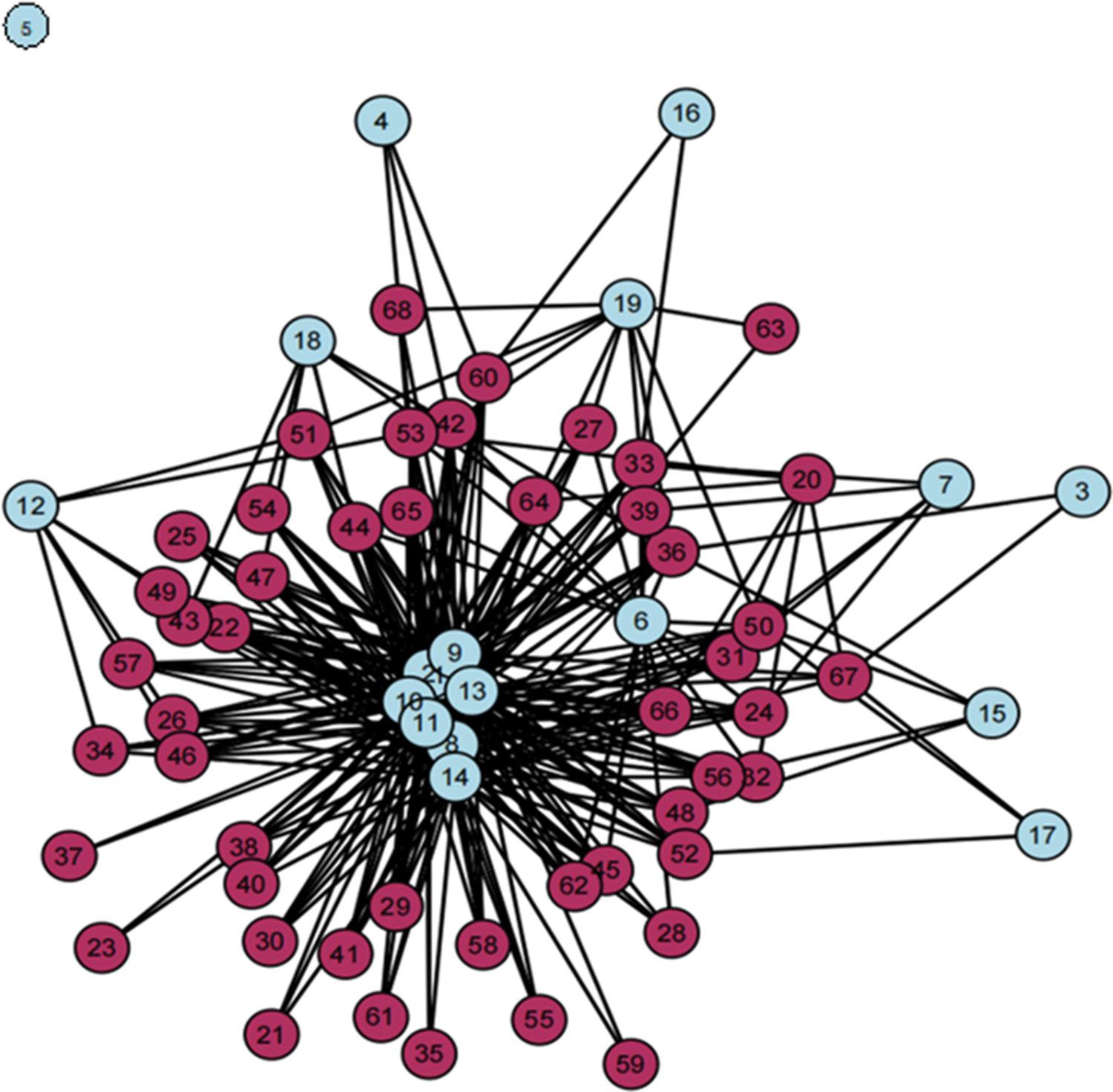
BCF-ISFL3ASAP1
CTF4AF2
FIP7GCCA8
GEF712GEF49
MDG AF15GEF510
PMR16GEF611
PPCR17GCF-IRM13
SREP18LDCF14
SCCF19
the country with the largest portion of climate finance, all coming from the CFUs (Figure 2).
To visualise the dynamic nature of the network, the filmstrip function in the ndtv R package was applied. It breaks the network up into successive temporal slices, giving us a view of the network as it develops over time (Figure 3). Hence, we get to see snapshots (that is, static plots) at a few key moments of the dynamic networks, over the lifetime of the projects. It can be observed that longer-term project networks tend to ‘mature’ (or transform) faster than 5-year or 3-year duration projects. There is a
persistent pattern of a sparse neighbourhood emerging around the year 2010 for the 3- and 5-year duration projects only. This pattern persists for a while up to the year 2014, for only short-term projects. In both the medium- and long-term projects, however, more dense subgroups can be observed in the latter years of formation where the transition behaviour from the year 2012 follows a similar pattern. Figure 4 denotes how centrality changes over time, year on year, based on the rolling aggregated betweenness centrality. This is an example of crucial node types which capture how much a specific node lies in between other nodes (serving as a key broker). It measures the fraction of the least paths that are passing through a given node. High values of betweenness centrality are generally used to identify vertices that preserve the whole network’s connectivity. The climate finance flow network (Figure 4) experienced its lowest dip around 2007, and although it has risen since then, it has not approached its 2004 peak (or thereabout). This suggests that the connectivity of the financial flows across sub-Saharan Africa was at its lowest during the period of the global financial crisis which started in 2007 and lasted until 2009, most probably because the major key players (donors) temporarily stopped or drastically reduced funding. By 2010, after the crisis, it had stabilised a bit, but was not yet fully recovered.
Decision tree analysis of climate finance flow
The theme/objective of the data set entries was used as a guide. The four themes are Mitigation General (Mitigation G for short), Adaptation, Mitigation REDD and Multiple foci. The amount of funding approved for each country under each specific theme was then extracted as shown in Table 4 (for the first 15 countries).
Overall, across the 48 sub-Saharan African countries, a total of USD1437.95 million has been approved for projects under the Mitigation G theme, USD2038.27 million for Adaptation, USD565.58 million for
Volume 120| Number 3/4 March/April 2024 56 https://doi.org/10.17159/sajs.2024/15837 Research Article Climate finance across sub-Sahara Page 4 of 12
Numeric
Figure 1: Static network based on climate fund transfer from multilateral funds (light blue) to different African countries (maroon).
Boundary funding units Numeric code (BFus) Central funding units
code (CFus)
table 3: Boundary and central multilateral funding units
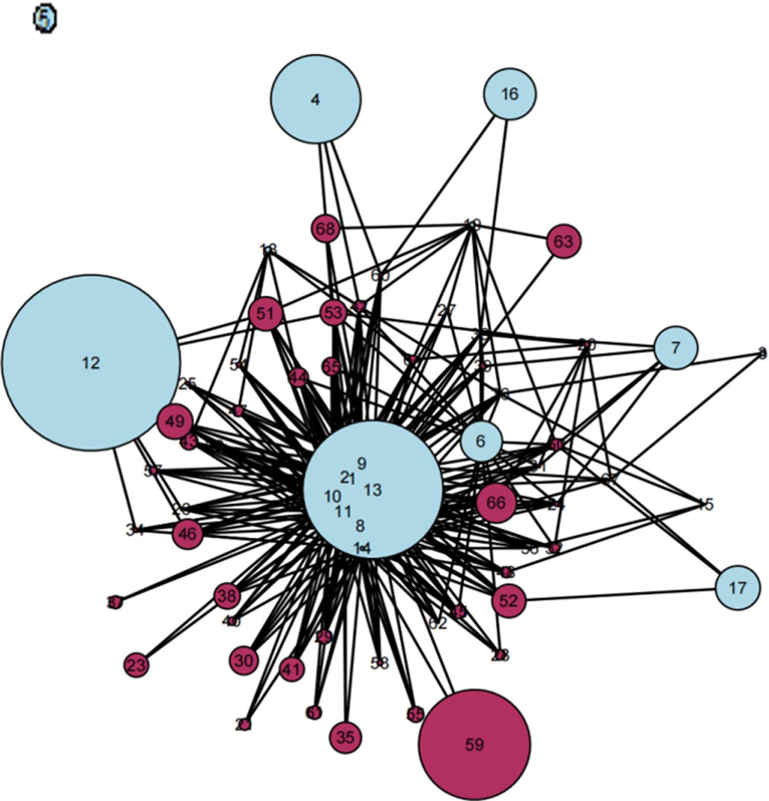
Mitigation REDD and USD383.85 million for projects leaning towards Multiple foci objective. This finding underlines the fact that mitigation finance dominates the total climate finance flowing into sub-Saharan Africa, as previously noted by Savividou et al.20 This is not a healthy path for the region. The summary statistics for each objective are denoted in Supplementary table 3
Setting region as the target variable, each variable’s univariate and bivariate distribution was examined with respect to the target variable using simple histogram representations. The R packages used in this analysis were plyr, dplyr, ggplot2, caret, rpart, rpart.plot, e1071 and stringi. The univariate distributions are displayed in Figure 5.
All the themes display right-skewed distributions and possess extreme outliers. Adaptation, however, is less skewed and there are fewer very high and low values in comparison with the other objectives. Most of the Mitigation G funds fall between 0 to USD100 million (Figure 5a). The bivariate distribution is created by converting the variable region to a factor variable where the region’s numeric code features are used to represent the factor levels. Region 1 refers to western Africa, region 2 southern Africa while central and eastern Africa are represented by regions 3 and 4, respectively. Each of the continuous variables (the themes) was then examined in relation to the target variable (Figure 6).
From Figure 6a, countries in region 3 (central Africa) are more likely to receive a higher proportion of Mitigation G finance if the projects fall within the range of USD100 million. However, the countries in region 2 (southern Africa) get a disproportionately high amount of Mitigation G funds as indicated by the extreme outlier. With Adaptation finance (Figure 6b), a
much more evenly distributed mechanism is at play (specifically when the funds are less than USD50 million). The histogram takes the form of a bimodal distribution, where the first mode is approximately normal. In the case of Mitigation REDD, an even distribution is also observed in general, with the exception that funds greater than USD100 million are more likely to go to countries in region 3 (Figure 6c). Finally, countries that fall under region 4 (eastern Africa) are more likely to receive higher Multiple foci climate finance if it is above USD25 million (Figure 6d). These patterns also speak loudly about the kinds of climate-related projects that are more dominant in a given sub-Saharan African region.
To further classify the themes of climate finance region-wise, decision trees were built. The plots are shown in Figure 7.
Train/test split approaches were implemented in the cases of Figure 7(b–d). One node remained unused in all cases, with the exception of Figure 7d where the leaf size was lowered. Although the test accuracy for the latter is lower than that in plot c, it will be adopted because it makes use of all the nodes (regions); however, Mitigation G is not used. It should be noted that these results may not be reliable enough, given the small sample size of 48 that was used. Figure 7d indicates that region 4 (eastern Africa) fully dominates when Adaptation finance is greater than USD55 million. This aligns with the bivariate plot in Figure 6b where we see region 4 showing up 4 out of 7 times when funds are greater than USD50 million and 1 out of 7 times when less than USD50 million. This finding was observed by Atteridge et al.29 as well. They expressed concerns over the concentration of Adaptation finance in only a small number of sectors, noting that this could hinder the broader impact of the objective.
Volume 120| Number 3/4 March/April 2024 57 https://doi.org/10.17159/sajs.2024/15837 Research Article Climate finance across sub-Sahara Page 5 of 12
Figure 2: Weighted static network of climate finance flows from multilateral funds (light blue) to different African countries (maroon). The approved funds serve as the weights.
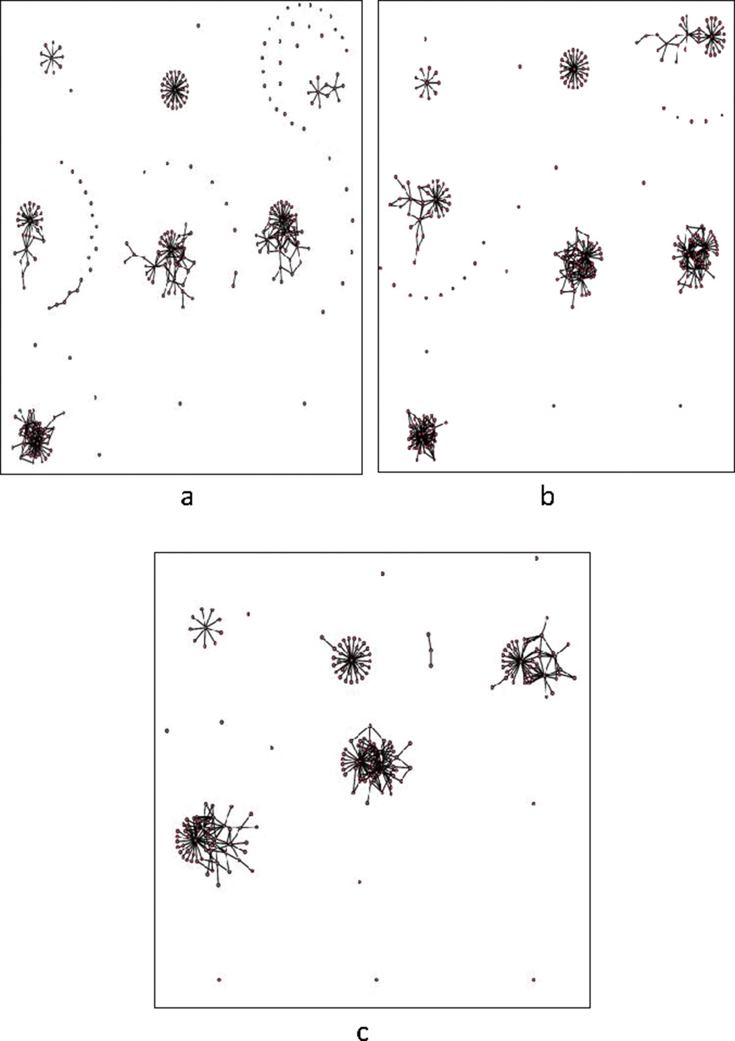
Region 2 (southern Africa) is characterised by lower (less than USD55 million) levels of Adaptation finance with projects under Mitigation REDD costing less than USD0.98 million, and for Multiple foci, less than USD5.1 million. Region 3 (central Africa), however, gets more than USD0.98 million with regard to Mitigation REDD, even though it receives less than USD55 million in Adaptation funds. Their Multiple foci quota share is much less (less than USD1.8 million).
Implications for practitioners, policymakers, donors and regulators
About 63% of the multilateral climate funding units (studied in this paper) are yet to disburse up to 50% of their approved funds for climate-related
projects in sub-Saharan Africa. This generally signifies the very slow pace at which the low-carbon, climate-resilient goal is being achieved. This is also a wake-up call to the African regions. More African regionalbased multilateral funding units are needed. Both the private and public sectors should be fully involved in coordinating such climate finance pools with the associated required regulations.
Implications from network analysis: The less dense region of the network reveals some sort of vulnerable position for the countries (up to 16 of them) located therein. With the exception of South Africa, which gulps in the largest share of climate funds, the others in the sparse region have to share what is left with the countries in the denser region. Secondly, this brings to the fore the issues surrounding equitable
Volume 120| Number 3/4 March/April 2024 58 https://doi.org/10.17159/sajs.2024/15837 Research Article Climate finance across sub-Sahara Page 6 of 12
Figure 3: The (a) 3-year, (b) 5-year and (c) 10-year duration of the temporal snapshots for the dynamic network. Moving across the rows (three in each case) from left to right, the times of occurrence of the static projections of the temporal networks are t= 2003, 2005.375, 2007.75, 2010.125, 2012.5, 2014.875, 2017.25, 2019.625, 2022 for (a); t=2003, 2005.625, 2008.25, 2010.875, 2013.5, 2016.125, 2018.75, 2021.375, 2024 for (b); and t=2003, 2006.25, 2009.5, 2012.75, 2016, 2019.25, 2022.5, 2025.75, 2029 for (c).
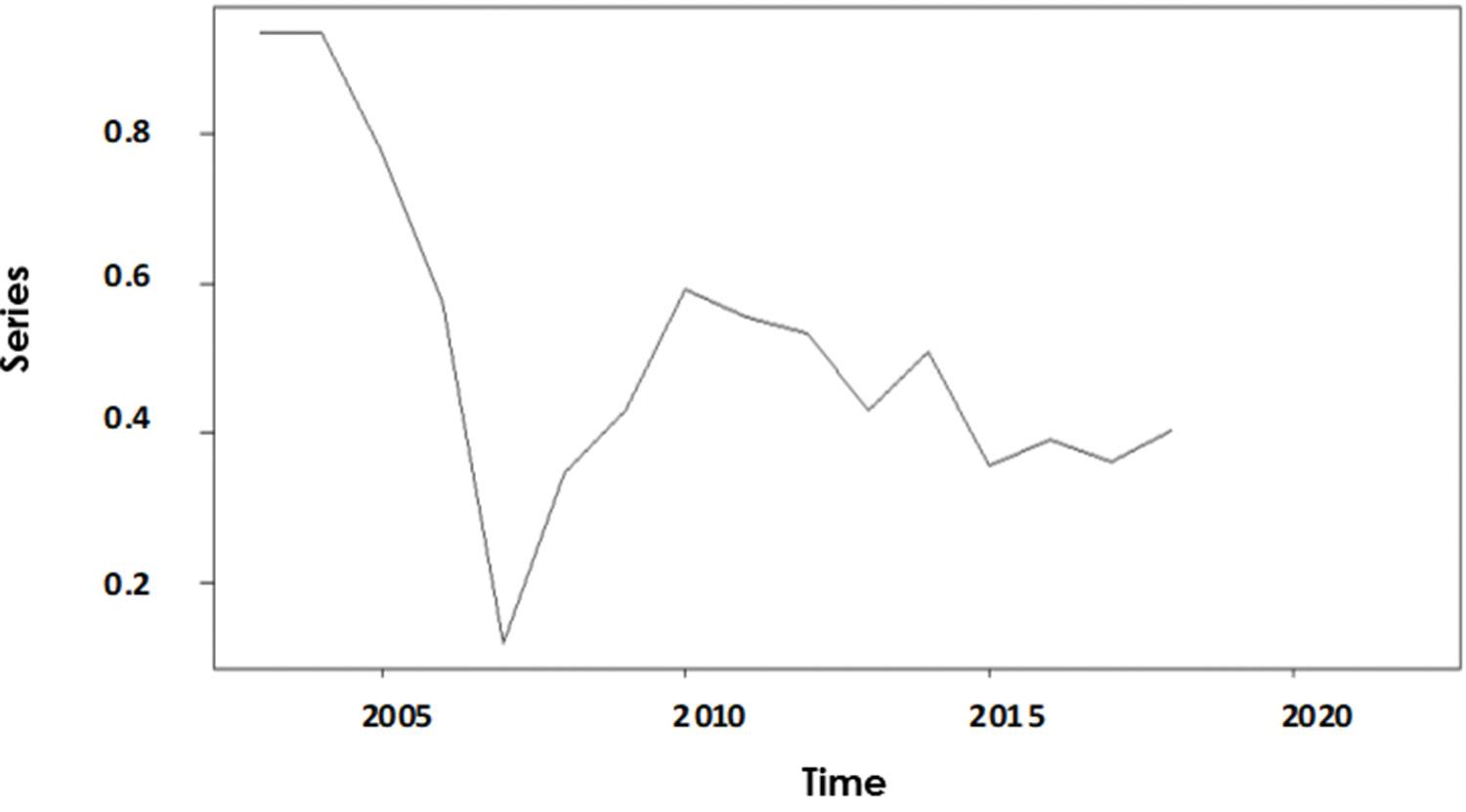
Countryregion region’s numeric code Mitigation G (uSD millions) Adaptation (uSD millions) Mitigation rEDD (uSD millions) Multiple foci (uSD millions)
AngolaSouthern
BotswanaSouthern Africa22.63000.95
Burkina
BurundiCentral
Cabo
ChadCentral
Congo,
Congo,
Cote
Equatorial
EritreaEastern
resource allocation of climate funds, given the scarcity of BFUs allocating funds to a number of African countries. A situation in which the CFUs are overburdened might ensue, leading to the unexpected accumulation of approved funds if this type of setup tarries for a long time. An example of such a situation might be during a financial crisis. In the absence of alternative (boundary) multilateral funding units, the isolated regions are bound to suffer the most.
It must also be noted that while South Africa is the largest emitter of carbon in Africa, hence requiring more climate funds (particularly mitigation finance), the climate change issue remains a global problem. The attainment of low carbon across African countries will as well impact South Africa positively, judging from the extremal dependence of climatic variables that may be present in African regions, eastern Africa
for example.30 This therefore implies that a fair balance for climate fund allocation needs to be struck by the donors. Thirdly, the presence of this gap presents opportunities for practitioners seeking to engage in the global/continental climate fund negotiation processes, as the entry of more multilateral funding units can help limit the monopolisation of African countries’ access to international funds. Fourthly, the structure of the network seems to suggest a greater coordination between CFUs than BFUs, although this may not be reflective of the real situation. Nevertheless, there is need for greater coordination between the funding units at the boundaries and at the centre to enable every African country to benefit from both sources.
Implications from decision tree analysis: Although eastern Africa is arguably the hardest hit region in terms of the adverse effects of climate
Volume 120| Number 3/4 March/April 2024 59 https://doi.org/10.17159/sajs.2024/15837 Research Article Climate finance across sub-Sahara Page 7 of 12
Figure 4: Year-on-year aggregated betweenness centrality changes for the temporal network.
Africa28.1625.6700
BeninWestern Africa17.5251.12.631.89
FasoWestern Africa129.6549.353.075.92
Africa33.422.8600
VerdeWestern Africa14.537.2808.12
Africa33.734.0313.990.34
African RepublicCentral Africa32.6510.127.60.63
CameroonCentral
Central
Africa34.9935.84014.64
Africa45.9169.9303.76
ComorosEastern
Replubic of Central Africa328.1526.86120.910.96
Democratic
Republic ofCentral Africa35.071022.780.66
d’IvoireWestern Africa18.356.3449.314.24
GuineaCentral
Africa34.360.25.930.9
Africa4015.7708.26
table 4: Approved funds for sub-Saharan African countries based on the themes
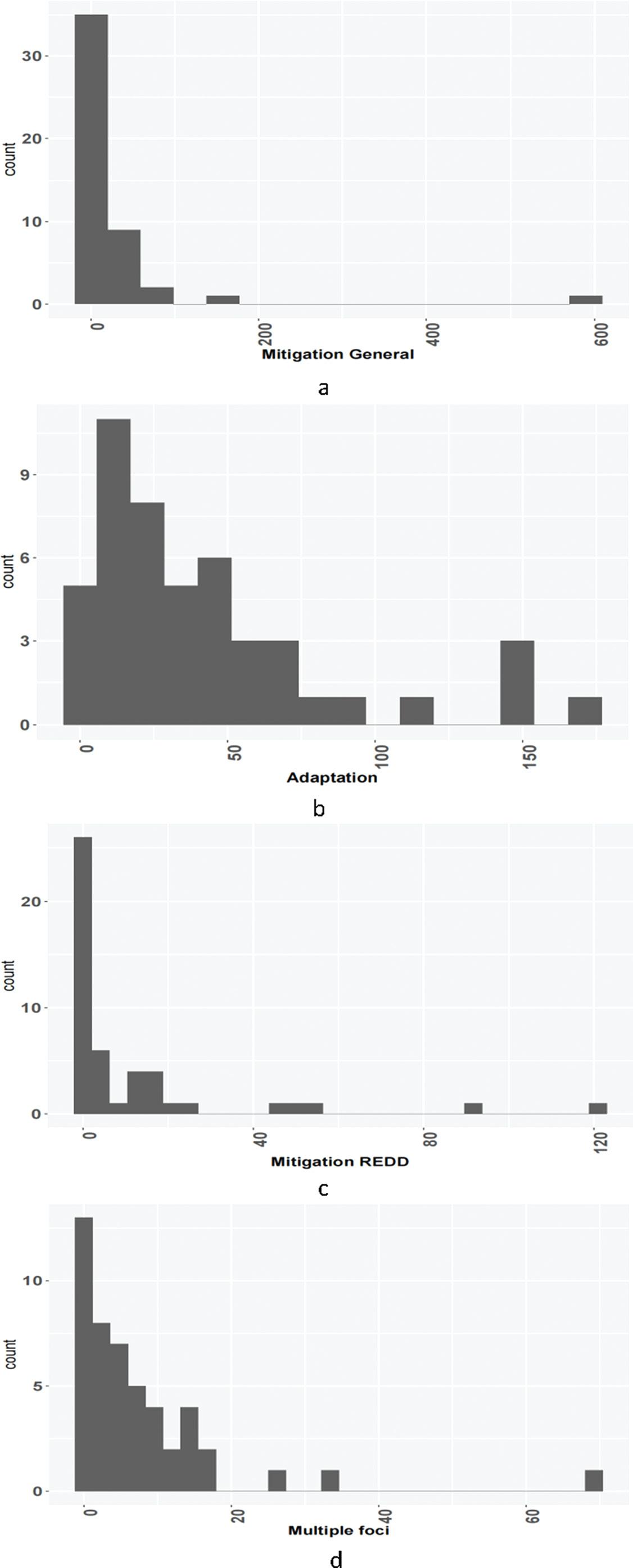
Volume 120| Number 3/4 March/April 2024 60 https://doi.org/10.17159/sajs.2024/15837 Research Article Climate finance across sub-Sahara Page 8 of 12
Figure 5: Univariate distributions of themes (a) Mitigation G, (b) Adaptation, (c) Mitigation REDD and (d) Multiple foci, with respect to the different African regions.
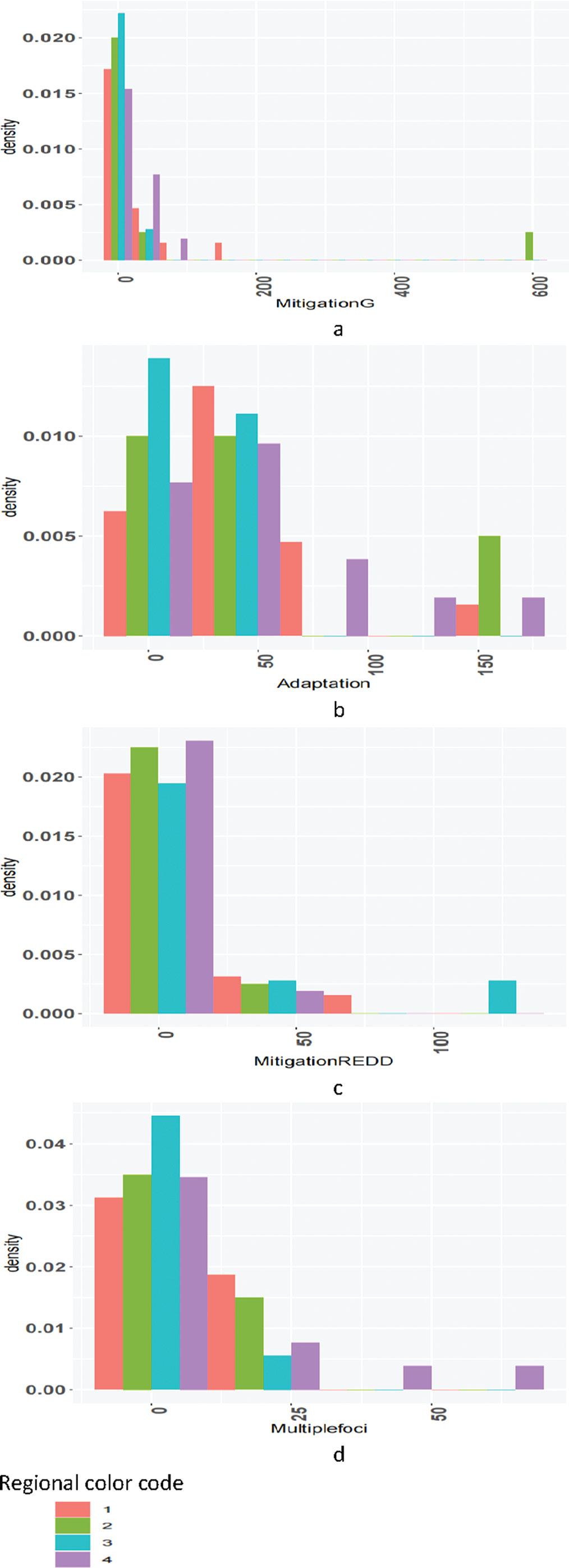
Volume 120| Number 3/4 March/April 2024 61 https://doi.org/10.17159/sajs.2024/15837 Research Article Climate finance across sub-Sahara Page 9 of 12
Figure 6: Bivariate distributions of themes with respect to the countries’ regions: western Africa = 1, southern Africa = 2, central Africa = 3, and eastern Africa = 4 in the colour-coded key.
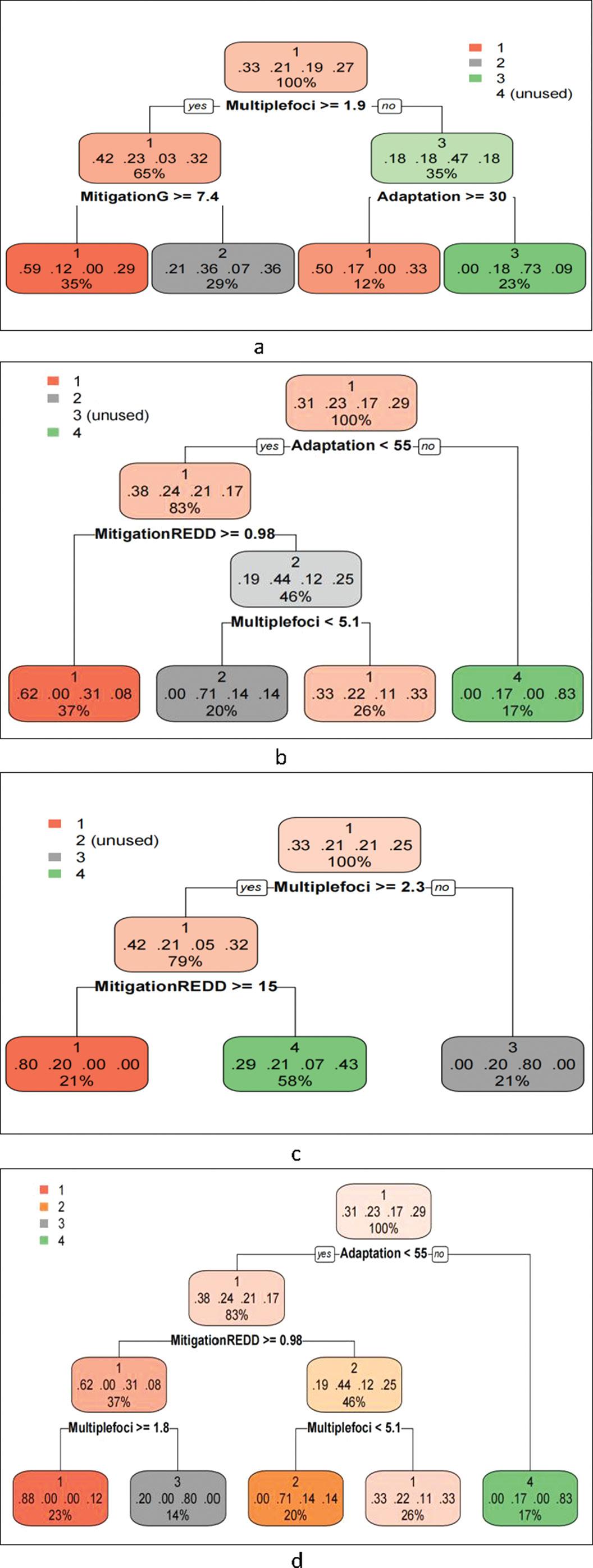
Volume 120| Number 3/4 March/April 2024 62 https://doi.org/10.17159/sajs.2024/15837 Research Article Climate finance across sub-Sahara Page 10 of 12
Figure 7: Decision trees classifying the climate finance themes region-wise. (a) No partition, (b) 70/30 partition with test data accuracy=7%, (c) 50/50 partition with test data accuracy=33%, (d) 70/30 partition with a lowered leaf size and test data accuracy=23%.
change in Africa, the highly unequal distribution of Adaptation finance for funds greater than USD50 million may be a matter of concern. This is due to the critical assistance other African countries currently need (particularly in the area of agriculture) in order to adapt to the rapid increase in the impacts of climate change already being experienced as a result of droughts and floods. Rapid desertification, for instance, lies at the base of the farmer–herder violence in northern Nigeria, which has since reached crisis levels, leading to the loss of thousands of lives and property, massive internal displacements, and heightened food insecurity.31-33 Adequate adaptation funds will definitely go a long way in resolving this problem (all else being equal).
Conclusion
Climate finance holds the key to obtaining the goals set for achieving a low-carbon world. However, the complexities involved in monitoring its flow across sub-Saharan Africa have not been thoroughly dealt with. This study was an in-depth critical look at how the flow is structured. The results obtained generally fit the multilateral funding units into two categories: the central and boundary funding units. Although more African countries have the opportunity of a boundary funding source which supplements the central source, a substantial number of countries remain in the isolated region at the boundary as they rely only on the central funding units, thus increasing their vulnerability. This vulnerability can become even more evident when shocks such as pandemics and financial crises are introduced into the system, as the flow of money declines significantly during such periods. Hence, there is a need for the major stakeholders in the concerned countries to highlight these issues when negotiating for climate finance. Plus, other alternatives can be prepared ahead of time because mitigation and adaptation strategies for climate change demand huge amounts of finance.
Nevertheless, further studies are required to understand the evolution of this vulnerable group when other climate funding sources are accounted for, such as multilateral, bilateral, grant-type, national and local government sources. Additionally, the diverse nature of the countries in Africa implies that each has their own special climate-related problems, risks, and solutions. The complexities of how climate money is distributed within individual countries and each country’s unique needs and efforts may be overlooked if countries are grouped into broad regional groupings. Other variables such as political links, past obligations, and the success of national climate policy also affect how climate financing is allocated. Hence, country-specific analyses of climate finance flows and their effects might offer a more perceptive viewpoint on the matter. To this end, African governments are encouraged to give keen attention to data collection and data storage. There is also a need to understand if there are any patterns emerging that differentiate projects into fully disbursed finance versus those that have partially disbursed finance, the regions affected and the reasons for failure to disburse funds.
Competing interests
I have no competing interests to declare.
references
1. UNFCCC. Introduction to climate finance [document on the Internet]. c2015 [cited 2022 Dec 10]. Available from: https://unfccc.int/topics/climate-financ e/the-big-picture/introduction-to-climate-finance
2. United Nations. 7d Paris agreement. United Nations Treaty Collection, chapter XXVII environment [document on the Internet]. c2016 [cited 2022 Dec 10]. Available from: https://treaties.un.org/Pages/ViewDetails.aspx?src=TREATY &mtdsg_no=XXVII-7d&chapter=27&clang=_en
3. Watson C, Schalatek L. The global climate finance architecture. Technical report ODI and HBS [document on the Internet]. c2020 [cited 2022 Nov 20]. Available from: https://climatefundsupdate.org/publications/the-global-climat e-finance-architecture-2018/
4. IPCC. Climate change 2014: Mitigation of climate change. Working Group III contribution to the Fifth Assessment Report of the Intergovernmental Panel on Climate Change. Cambridge, UK: Cambridge University Press; 2014. https://doi. org/10.1017/CBO9781107415416
5. IPCC. Chapter outline of the Working Group III contribution to the IPCC Sixth Assessment Report (AR6) (forty-sixth session of the IPCC) [document on the Internet]. c2017 [cited 2022 Dec 20]. Available from: https://www.ipcc.ch/si te/assets/uploads/2018/03/AR6_WGIII_outlines_P46.pdf
6. Thomson I, Charnock R. Engaging with the IPCC on climate finance. A call to actionandplatformforsocialandenvironmentalaccountingscholars.SocEnviron Account J. 2022;42(1). https://doi.org/10.1080/0969160X.2022.2085131
7. Banga J. Essays on climate finance [doctoral thesis]. Grenoble: Grenoble Alpes University; 2020. Available from: https://hal-emse.ccsd.cnrs.fr/CREG /tel-02954765v1
8. Bird N, Brown J, Schalatek L. Design challenges for the Green Climate Fund. Climate finance policy brief 4 [document on the Internet]. c2011 [cited 2023 Jan 22]. Available from: https://odi.cdn.ngo/media/documents/6457.pdf
9. Steckel JC, Jakob M, Flachsland C, Kornek U, Lessmann K, Edenhofer O. From climate finance toward sustainable development finance. Clim Change. 2016;8(1). https://doi.org/10.1002/wcc.437
10. Bowen A. Raising climate finance to support developing country action: Some economic considerations. Clim Policy. 2011;11(3):1020–1036. http s://doi.org/10.1080/14693062.2011.582388
11. Carraro C, Massetti E. Beyond Copenhagen: A realistic climate policy in a fragmented world. Clim Change. 2012;110(3):523–542. https://doi.org/10. 1007/s10584-011-0125-6
12. Buchner B, Brown J, Corfee-Morlot J. Monitoring and tracking long-term finance to support climate action [document on the Internet]. c2011 [cited 2023 Jan 22]. Available from: https://www.oecd.org/environment/cc/48073739.pdf
13. Clapp C, Ellis J, Benn J, Corfee-Morlot J. Tracking climate finance: What and How? Paris: OECD Publishing; 2012. https://doi.org/10.1787/5k44xwt k9tvk-en
14. Donner S, Kandlikar M, Webber S. Measuring and tracking the flow of climate change adaptation aid to the developing world. Environ Res Lett. 2016;11(5), Art. #054006. https://doi.org/10.1088/1748-9326/11/5/054006
15. Grasso M. The role of justice in the North–South conflict in climate change: The case of negotiations on the Adaptation Fund. In: International environmental agreements: Politics, law and economics. Dordrecht: Springer; 2011. p. 361–377. https://doi.org/10.1007/s10784-010-9145-3
16. Soltau F. Fairness in international climate change law and policy. Cambridge, UK: Cambridge University Press; 2009. https://doi.org/10.1017/CBO97805 11635403
17. Zhang W, Pan X. Study on the demand of climate finance for developing countries based on submitted INDC. Adv Clim Chang Res. 2016;7(2). https:/ /doi.org/10.1016/j.accre.2016.05.002
18. Bowen A, Campiglio E, Martinez SH. The optimal and equitable climate finance gap [document on the Internet]. c2015 [cited 2023 Jan 22]. Available from: https://www.lse.ac.uk/granthaminstitute/wp-content/uploads/2015/03 /Working-Paper-184-Bowen-et-al.pdf
19. Halimanjaya A. Climate mitigation finance across developing countries: What are the major determinants? Clim Policy. 2015;15(2). https://doi.org/10.108 0/14693062.2014.912978
20. Savvidou G, Atteridge A, Omari-Motsumi K, Trisos CH. Quantifying international public finance for climate change adaptation in Africa. Clim Policy. 2021;21(8):1020–1036. https://doi.org/10.1080/14693062.2021.1978053
21. Doku I, Ncwadi R, Phiri A. Determinants of climate finance: Analysis of recipient characteristics in sub-Saharan Africa. Cogent Econ Finance. 2021;9(1), Art. #1964212. https://doi.org/10.1080/23322039.2021.1964212
22. Chukwudum QC, Nadarajah S. Modelling climate finance flows in SubSaharan Africa. Environ Model Assess. 2023;28:977–998. https://doi.org/10 .1007/s10666-023-09923-z
23. Bird N, Watson C, Schalatek L, Keil K. Climate finance regional briefing: SubSaharan Africa. Climate finance fundamentals 7 [document on the Internet]. c2017 [cited 2023 Jan 22]. Available from: https://climatefundsupdate.org/w p-content/uploads/2022/03/CFF7-Sub-Saharan-Africa_ENG-2021.pdf
24. Watson C, Schalatek L. Climate finance thematic briefing: Adaptation finance [document on the Internet]. c2020 [cited 2023 Jan 29]. Available from: ht tps://climatefundsupdate.org/publications/the-global-climate-finance-archite cture-2018/
Volume 120| Number 3/4 March/April 2024 63 https://doi.org/10.17159/sajs.2024/15837 Research Article Climate finance across sub-Sahara Page 11 of 12
25. Hirsch T. A resource guide to climate finance: An orientation to sources of funds for climate change programmes and action [document on the Internet]. c2018 [cited 2023 Jan 22]. Available from: https://actalliance.org/wp-conten t/uploads/2018/06/ENGLISH-quick-guide-climate-finance.pdf
26. Hevey D. Network analysis: A brief overview and tutorial. Health Psycho Behav Med. 2018;6(1):301–328. https://doi.org/10.1080/21642850.2018.1521283
27. KotsiantisSB.Decisiontrees:Arecentoverview.ArtifIntellRev.2013;39:261–283. https://doi.org/10.1007/s10462-011-9272-4
28. Watson C, Schalatek L. Climate finance thematic briefing: Mitigation finance [document on the Internet]. c2020 [cited 2023 Jan 29]. Available from: ht tps://climatefundsupdate.org/publications/the-global-climate-finance-archite cture-2018/
29. Atteridge A, Savvidou G, Canales N, Verkuijl C. UNFCCC Standing Committee on Finance. Call for evidence: Information and data for the preparation of the 2020 biennial assessment and overview of climate finance flows [document on the Internet]. c2020 [cited 2023 Jan 29]. Available from: https://unfccc.in t/sites/default/files/resource/Call_for_evidence_2020BA.pdf
30. Chukwudum QC. Insuring against drought. In: The end of normal how climate change affects weather patterns and what to do about it. A compendium of essays for the Allianz Climate Risk Research Award. Munich: Allianz; 2019. p. 108–152.
31. Olesin SI, Munonye JO, Onyeneke RU, Adefalu LL, Olaolu MO, Azuamairo GC, et al. Farmer-herders’ conflict and climate change: Response strategies needed in Nigeria and other African countries. Int J Clim Change: Impacts responses. 2021;14(1):73–89. https://doi.org/10.18848/1835-7156/CGP/v14i01/73-89
32. Ojekunle A. Here are the 14 most affected states by Nigeria’s farmer-herder conflicts [document on the Internet]. c2018 [cited 2023 Feb 12]. Available from: https://www.pulse.ng/bi/politics/here-are-the-14-states-most-affected-by-nigeri as-farmer-herder-conflicts/3cz15p8
33. AzareIM,AbdullahiMS,AdebayoAA,DantataIJ,DualaT.Deforestation,desert encroachment, climate change and agricultural production in the SudanoSahelian region of Nigeria. J Appl Sci Environ Manage. 2020;24(1):127–132. https://doi.org/10.4314/jasem.v24i1.18
Volume 120| Number 3/4 March/April 2024 64 https://doi.org/10.17159/sajs.2024/15837 Research Article Climate finance across sub-Sahara Page 12 of 12
AuthorS:
Jacobus A. Kruger1
Sarah J. Roffe1,2
Adriaan J. van der Walt1,3
AFFILIAtIoNS:
1Department of Geography, University of the Free State, Bloemfontein, South Africa
2Agrometeorology Division, Agricultural Research Council –Natural Resources and Engineering, Pretoria, South Africa
3Afromontane Research Unit, Faculty of Natural and Agricultural Sciences, University of the Free State, Bloemfontein, South Africa
CorrESPoNDENCE to:
Adriaan van der Walt
EMAIL:
vanderwalta@ufs.ac.za
DAtES:
received: 26 Apr. 2023
revised: 14 Sep. 2023
Accepted: 08 Nov. 2023
Published: 27 Mar. 2024
hoW to CItE:
Kruger JA, Roffe SJ, van der Walt AJ. AgERA5 representation of seasonal mean and extreme temperatures in the Northern Cape, South Africa.
S Afr J Sci. 2024;120(3/4), Art. #16043. https://doi.org/10.17159/ sajs.2024/16043
ArtICLE INCLuDES:
☒ Peer review
☒ Supplementary material
DAtA AVAILABILItY:
☐ Open data set
☐ All data included
☒ On request from author(s)
☐ Not available
☐ Not applicable
EDItor:
Jemma Finch
KEYWorDS:
heat waves, cold waves, AgERA5 reanalysis, weather stations, data set evaluation
FuNDING:
Society of South African Geographers; University of the Free State
AgERA5 representation of seasonal mean and extreme temperatures in the Northern Cape, South Africa
Over regions with sparse observation networks, including South Africa’s Northern Cape Province, gridded data sets represent valuable supplementary data sources enabling spatially detailed climate investigations. Their performance is, however, influenced by regional characteristics, thus a performance assessment should be a prerequisite for any regional application. Through a pairwise comparison with eight point-based temperature records, we evaluated the AgERA5 data sets representation of mean summer (November–March; Tms) and winter (May–September; Tmw) temperatures and respective seasonal heatwave and coldwave characteristics across the Northern Cape for 1980–2020. Correlations ranging from 0.48 to 0.92 for Tms and from 0.38 to 0.94 for Tmw reflect relatively strong, but varying, temporal correspondence between the AgERA5 data and stations. Low biases, averaging 0.08 (0.17) °C and ranging from -0.79 to 2.10 (-0.40 to 1.47) °C for Tms (Tmw) were evident. Biases for the heatwave (coldwave) magnitudes were low, averaging -0.38 (0.19) °C2 , and ranging from -1.55 to 1.47 (-2.05 to 2.91) °C2. Biases for the heatwave (coldwave) frequency were also low, but typically overestimated, averaging 1.19 (0.73) days, and ranging from -1.33 to 5.60 (-1.61 to 3.39) days. Biases for the heatwave (coldwave) number were low and typically overestimated, averaging 0.27 (0.08) events, and ranging from -0.28 to 1.40 (-0.39 to 0.39) events. Despite some stations depicting consistently poor performance, the study results support further application of the AgERA5 product for spatiotemporal analyses of mean and extreme temperatures across the Northern Cape, provided limitations are adequately acknowledged. Further application of the fine-resolution AgERA5 product will greatly inform impact-based studies exploring mean and extreme temperature influences over the Northern Cape Province.
Significance:
• The AgERA5 product was assessed on its performance in representing average and extreme temperature characteristics over South Africa’s Northern Cape Province.
• Good comparability between the AgERA5 product and point-based observations supports further application of the AgERA5 across the Northern Cape.
• The AgERA5 product offers a spatially detailed picture of mean and extreme temperatures across the Northern Cape, which is valuable for regions where weather stations are not available.
• The AgERA5 product is thus important for impact-based studies assessing, for instance, the impact of extreme temperatures on livestock and human health.
Introduction
Southern Africa is expected to experience above global-average warming, which will lead to drastic changes in regional extreme temperature event (ETE) characteristics.1-3 Historical trends and future projections indicate that, compared to other South African provinces, the Northern Cape Province (Figure 1) has and will likely continue to experience among the largest increases in surface air temperature and hot ETE characteristics (e.g. heatwaves).1,4 Conversely, historical trends and future projections over southern Africa typically show decreasing trends in the cold ETE characteristics (e.g. coldwaves).5-7 During ETEs, prolonged exposure to thermal stress can have devastating impacts which can influence agricultural productivity, by reducing crop yields and potentially causing livestock mortalities, and human health, by exacerbating illnesses (e.g. headaches and asthma) and potentially leading to mortality.7-9 These impacts are of concern, because in developing regions, such as the Northern Cape, associated implications are exacerbated due to a high reliance on weather and climate-sensitive activities (e.g. agriculture), and high levels of poverty and unemployment.10,11
Across the Northern Cape Province, interactions between tropical, temperate and subtropical weather systems, the regional topography, and the cold Benguela Current (and the Benguela Upwelling System) are known to drive the occurrences of cold and hot ETEs.12 Through westerly troughs, cut-off lows and mid-latitude cyclone cold fronts, the mid-latitude westerlies and cold Benguela current (and the Benguela Upwelling System) contribute to the advection of cold air, from the southern Atlantic Ocean, over the Northern Cape and are known to be associated with cold snaps and coldwave events.12-14 Typically, heatwaves are associated with mid-to-lower tropospheric highpressure systems, limited cloud coverage, and enhanced incoming longwave radiation.15,16 Troughs extending from the tropics transport warm air from the farther northern tropical regions and are also known to induce hot ETEs across South Africa and the Northern Cape.17-19
Weather station records have been the primary data source for investigations regarding ETEs across South Africa, yet large parts of South Africa, especially mountainous and remote regions, have sparse station network coverage.20 Thus, station data alone cannot provide detailed spatial pictures required for climate studies. Station data sometimes have data quality issues and are not typically temporally complete due to technical issues and, in some cases, closure of stations.20 There is thus an increasing need for an alternative, or supplementary data
Research Article
65 https://doi.org/10.17159/sajs.2024/16043 Volume 120| Number 3/4 March/April 2024 © 2024. The Author(s). Published under a Creative Commons Attribution Licence.
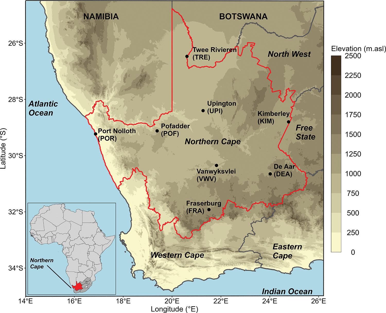
source, and gridded data sets offer such an alternative.21,22 Various gridded temperature data sets exist which are generated using different methods, such as interpolating station data, analysing satellite imagery, and assimilating observations from stations and/or satellite imagery through simulations.23-27 There is, however, uncertainty as to whether gridded data accurately represent temperature and ETEs, especially in regions adjacent to oceans, with steep near-surface temperature gradients, elevation gradients and/or precipitation gradients.21,22 The Northern Cape represents a region with steep elevation gradients, where the high-lying interior plateau and low-lying coastal plain are separated by the mountainous region of the western Great Escarpment (Figure 1). The Northern Cape has a complex rainfall climatology, with a summer rainfall zone towards the east, a year-round rainfall zone from the central parts to the edge of the western Great Escarpment, and a winter rainfall zone across the coastal plain.28 Therefore, over a region like the Northern Cape, a fine resolution data set should provide a more detailed representation of the region’s climate, as studies demonstrate that finer resolution data sets often, but not always, provide improved climate representations compared to coarser products.20,29
Among the available gridded temperature products, the ERA5, and specifically products downscaled from it (i.e. AgERA5), offer the highest resolution temperature data sets.25,26 Although recent research has assessed the AgERA5 data set in representing mean and extreme temperatures across the Northern Cape, a gridded observation-based product was considered. Thus, there is still uncertainty as to whether the AgERA5 area-averaged grid cells accurately compare to pointbased temperature records.20 Therefore, using point-based weather station records from the South African Weather Service (SAWS), we aimed to apply comparative statistics to explore the performance of the AgERA5 data set in representing mean summer (Tms) and winter (Tmw) temperatures and respective seasonal heatwave and coldwave characteristics across the Northern Cape for 1980–2020. Considering the adverse implications associated with ETEs and the importance of reliable gridded data sets for spatial investigations of ETEs, the evaluation of such a data set is relevant as a prerequisite for further studies utilising the AgERA5 product over the Northern Cape.29
Data and methods
Data and pre-processing
The AgERA5 daily maximum and minimum temperature (Tx and Tn, respectively) outputs for 1980–2020 were utilised for this study; AgERA5 data are freely available for download from the Copernicus Climate Data Store.26 The AgERA5 data set is a statistically downscaled and bias-corrected product that is available at a 0.1° resolution.26 It is derived from the hourly ERA5 reanalysis which is available at a 0.25° resolution and combines numerical model, satellite and observation data using the European Centre for Medium-Range Weather Forecasts’ Integrated Forecast System (ECMWF).25,26 Before calculating the temperature indices using the AgERA5 data, several pre-processing steps were undertaken to prepare the data using the Climate Data Operators software.30 This preparation included the temporal merging of daily NetCDF files, spatial clipping to the study domain extent (i.e. 25–33° S and 17–25°E), converting units from K to °C, and changing of variable names according to the Climpact user manual.31
To evaluate the performance of the AgERA5 data set across the Northern Cape, daily Tx and Tn spanning 1980–2020 were utilised from eight SAWS weather stations (Supplementary table 1), purposively selected following van der Walt and Fitchett32, to produce an evenly distributed network of stations across the province (Figure 1). For inclusion, stations were required to have >90% data availability for 1980–2020.33 Before statistical analyses, data quality was examined and cleaning was performed.32,33 All dates were checked for duplication and gaps, and values were rounded to two decimal places for consistency.33 Repetition and duplication of temperature values and where Tx ≤ Tn were among the errors identified, while outliers were identified using box plots and then verified through comparison with nearby stations.28,32,33 All errors and outliers identified were deleted and recorded as missing values.28,34,35 Missing values were filled with data from nearby stations if they were located within a 50 km radius and had a Spearman Correlation Coefficient (CC) of >0.70 between the existing records of both stations.32,35-37 If there were still missing values for less than five consecutive days, a fiveday running average was used to estimate these.28,32
Volume 120| Number 3/4 March/April 2024 66 https://doi.org/10.17159/sajs.2024/16043 Research Article Evaluation of AgERA5 temperature data across the Northern Cape Page 2 of 13
Figure 1: Study site map depicting elevation, neighbouring countries and provinces, bordering oceans, and locations of weather stations used across the Northern Cape Province. Details of the weather stations are presented in Supplementary table 1.
Heatwave and coldwave indices
To calculate ETE indices we utilised the R Climpact package, developed by the World Meteorological Organisation (WMO) Expert Team on Sectorspecific Climate Indices (ET-SCI).31 Among the available heatwave and coldwave definitions, the Excess Heat Factor (EHF) and excess cold factor (ECF) were applied herein for the heatwave and coldwave calculations for the extended summer (November–March) and winter (May–September) seasons for 1980–2020, respectively.38,39 The EHF/ ECF incorporates two components based on average daily temperatures, representing acclimatisation and significance, which are combined into one factor: the EHF/ECF.39 Heatwaves (coldwaves) are defined when the EHF (ECF) value is positive (negative) for at least three consecutive days.31,39 More information about the EHF, ECF and respective heatwave and coldwave calculations are detailed in Herold and McComb31 and Nairn and Fawcett.39
Duration, magnitude and frequency are heatwave and coldwave characteristics frequently used to describe such events.4,6,38 40 Thus, similar heatwave and coldwave indices were computed as seasonally averaged outputs for the AgERA5 and SAWS data sets. These include: (1) heatwave (coldwave) frequency (HWF [CWF]) which represents the total number of days contributing to annual summer (winter) heatwave (coldwave) events, (2) heatwave (coldwave) magnitude (HWM [CWM]) represents the average temperature of summer (winter) heatwaves (coldwaves) per year, measured as °C2 due to the EHF (ECF) definition and (3) heatwave (coldwave) number (HWN [CWN]) which represents the total number of summer (winter) heatwave (coldwave) events per year.38 39
Evaluation analysis
To evaluate the AgERA5 in representing Tms and Tmw, and respective seasonal ETE characteristics, we first explored the data sets’ performance in characterising daily average Tms and Tmw, using the summer and winter periods for the heatwave and coldwave calculations. Tms and Tmw are fundamental as they can dictate underlying factors influencing the performance of seasonal ETE characteristics.20 Thereafter, performance was explored for the respective ETE indices.
In all instances, four pairwise statistical metrics were calculated to compare the AgERA5 and SAWS data sets; single grid cell values corresponding to the station coordinates were extracted to compute the evaluation metrics (Supplementary table 1). CC was used to measure the level of temporal consistency between the AgERA5 and SAWS data sets, where output values range between zero and one, and one is optimal.28 Information on the standard metric errors, measuring deviation between the data sets, were calculated as Root Mean Square Error (RMSE) values, where outputs range between zero and one, with zero as the strongest score.22 The bias metric was used to determine the tendency of the AgERA5 data set to overestimate or underestimate values compared to the SAWS data set, where positive (negative) bias values indicate an overestimation (underestimation) by the AgERA5 data set, while a value of zero is optimal.41 The Modified Index of Agreement (MD) was used to identify both additive and proportional disparities in the SAWS and AgERA5 mean and variance ranges.42 43 This provides a valuable skill score for the data; the resulting value ranges between zero and one, with one being the desired value.42,43
results
AgERA5 representation of mean summer and winter temperatures
Box plots illustrating the distribution of Tms and Tmw across the weather stations and AgERA5 grid cells in the Northern Cape for 1980–2020 indicate that there is strong agreement between the data sets, with mean values deviating by <1 °C for most locations (excluding POR; Figure 2a–b). Excluding POR, the overlapping boxplot boxes for the stations and AgERA5 cells further indicate a high degree of agreement and strong correspondence between the two data sets (Figure 2a–b). For Tms, the box plots reveal that KIM and POR exhibit higher temperature values (i.e. warm bias) in the AgERA5 data set, whereas the remaining locations exhibit lower temperatures (i.e. cool bias; Figure 2a). This pattern is indicative of a predominant negative (cool) bias in the AgERA5 Tms proxies, which is apparent in the Supplementary figure 1 time series plots and the bias values (Table 1). Similarly, for Tmw, the box plots
Volume 120| Number 3/4 March/April 2024 67 https://doi.org/10.17159/sajs.2024/16043 Research Article Evaluation of AgERA5 temperature data across the Northern Cape Page 3 of 13
IndexStationCCMDrMSEBias Tms DEA 0.92 0.790.34-0.21 FRA 0.86 0.460.87-0.79 KIM 0.85 0.720.510.08 POF 0.90 0.700.38-0.26 POR 0.48 0.212.192.10 TRE 0.68 0.570.76-0.50 UPI 0.84 0.580.52-0.36 VWV 0.85 0.450.79-0.70 Tmw DEA 0.84 0.640.52-0.40 FRA 0.84 0.710.41-0.11 KIM 0.70 0.560.700.49 POF 0.94 0.720.57-0.29 POR 0.38 0.231.571.47 TRE 0.68 0.510.740.52 UPI 0.78 0.680.37-0.16 VWV 0.84 0.640.40-0.27
table 1: Tabulated results, per location mapped in Figure 1, of the comparison between the AgERA5 and SAWS data sets for average daily summer temperatures (Tms) and daily winter temperatures (Tmw). CC represents the Spearman Correlation Coefficient; RMSE represents the Root Mean Square Error; MD represents the Modified Index of Agreement. CC values denoted in bold represent statistically significant correlations at the 5% alpha level.
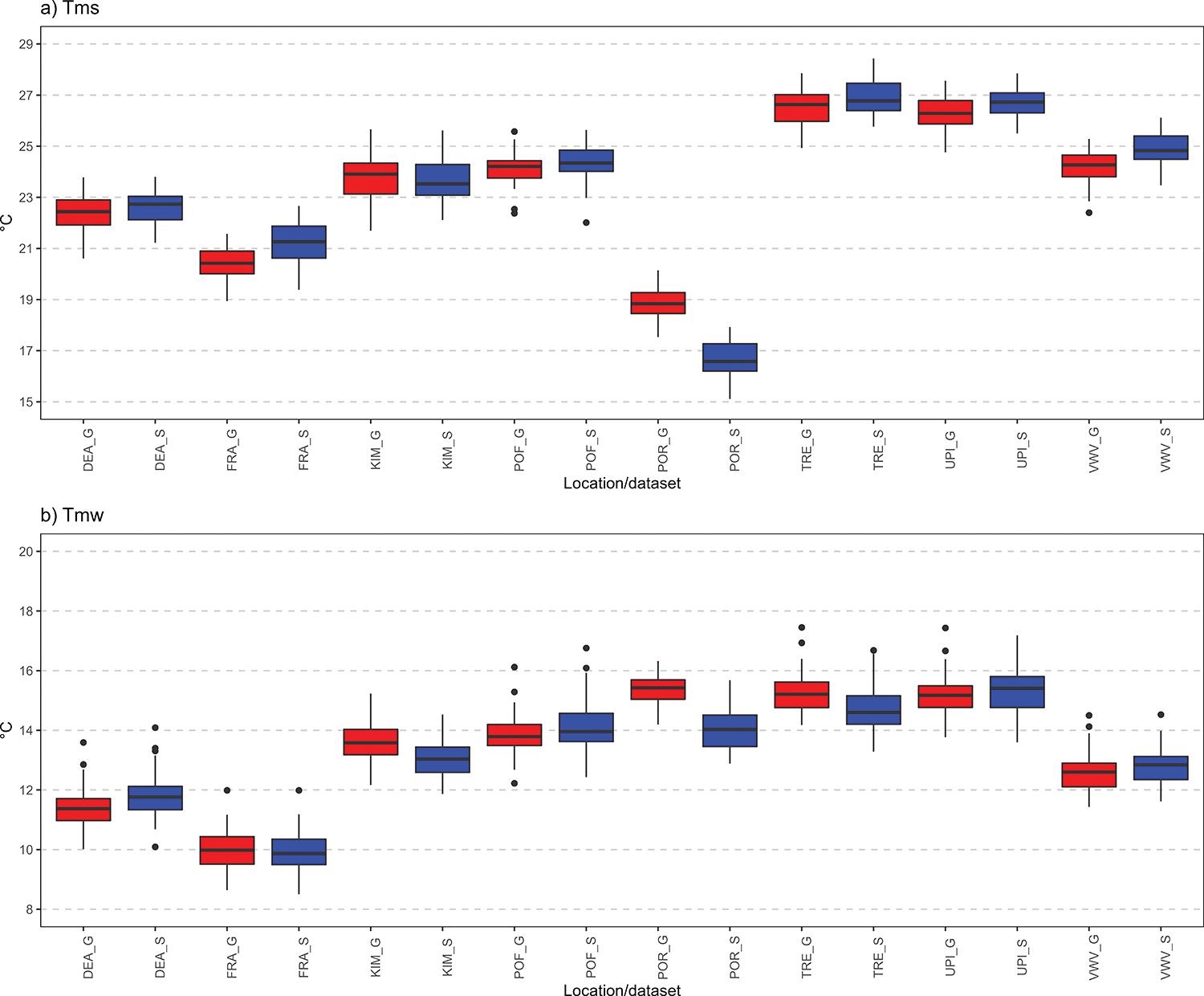
reveal that the AgERA5 cells exhibit higher temperatures (i.e. warm bias) at KIM, POR and TRE, while lower temperatures (i.e. cool bias) are observed at the remaining locations (Figure 2b). This indicates a predominant negative (i.e. cool) bias in the AgERA5 Tmw data, which is also evident in the time series plots and tabulated bias values (Table 1; Supplementary figure 1). Compared to SAWS data, most locations depict lower AgERA5 box plot tail ends, which may translate to an underestimation of AgERA5 extremetemperatures (Figure 2). Among the stations, POR consistently depicts weaker correspondence as mean values deviate by >1 °C and the spread of the data does not overlap consistently for both Tms and Tmw (Figure 2).
Strong temporal consistency between the AgERA5 and station data sets is supported by the statistically significant CC values, demonstrating consistent interannual variability patterns, and the time series plots, which demonstrate consistent temporal tracking between the two data sets (Supplementary figures 1 and 2; Table 1). The CC values are moderate to strong in magnitude, further indicating strong consistency between the data sets (Table 1). CC values range between 0.48 (POR) and 0.92 (DEA) for Tms and from 0.38 (POR) to 0.94 (POF) for Tmw, with stronger temporal correspondence for Tms as reflected by higher correlation values for most stations (Table 1). Located along the western coast and farthest north, POR and TRE exhibit the lowest degree of temporal agreement for Tms (Tmw), with CC values of 0.48 (0.68) and 0.38 (0.68), respectively (Table 1). The MD values further indicate strong agreement between the data sets, with Tms values ranging between 0.21 (POR) and 0.79 (DEA) and Tmw values from 0.23 (POR) to 0.72 (POF; Table 1). The low, but varying, deviation in seasonal temperatures between SAWS and AgERA5 for Tms is characterised by RMSE values ranging from 0.34 °C (DEA) to 2.19 °C (POR), while for Tmw RMSE values range from 0.37 °C (UPI) to 1.57 °C (POR; Table 1). The AgERA5 Tms values are overestimated by 0.08 °C and 2.10 °C at KIM and POR, respectively, and Tmw values are overestimated by 0.49 °C, 1.47 °C and 0.51 °C at KIM, POR and TRE, respectively (Table 1). In general, for most stations, the AgERA5 data set underestimates Tms and Tmw, as evidenced by the mostly negative bias values and the time series plots per station (Table 1;
Supplementary figures 1 and 2). Specifically, bias values range from -2.10 (POR) to 0.79 °C (FRA) for Tms and from -1.47 (POR) to 0.40 °C (DEA) for Tmw (Table 1). Despite these biases, their magnitudes are relatively small, which is consistent with the low RMSE values evident across the stations (excluding POR; Table 1).
AgERA5 representation of mean summer season heatwave characteristics
Box plots depicting the distribution of heatwave characteristics and time series plots illustrating temporal patterns across the stations and corresponding AgERA5 grid cells in the Northern Cape for 1980–2020 depict strong consistency between the data sets, as is evident from the overlapping boxes of the box plots, similar temporal variability patterns and consistent tracking for each time series (Figures 3–5; Supplementary figure 3). Specifically, the box plots indicate that most locations deviate, based on mean values, by <3 days for HWF, <1 °C2 for HWM and <1 event for HWN (Supplementary figure 3). However, the box plots of heatwave characteristics at different locations show different degrees of overlap, less so for POR, suggesting that the data distributions for these variables differ across various locations and characteristics (Supplementary figure 3).
Moderate to strong statistically significant CC values (>0.5) for all heatwave characteristics supports that there is strong agreement between the AgERA5 and SAWS data sets (Table 2). For HWF, CC values range from 0.60 (TRE) to 0.87 (KIM), while for HWM, CC values range from 0.53 (POR) to 0.93 (VWV), and HWN CC ranges are from 0.53 (POR) to 0.85 (KIM; Table 2). CC values for POR, UPI and TRE are generally weaker for all heatwave characteristics (Table 1). This observation is consistent with relatively little overlap observed between the corresponding boxplot boxes and weaker MD values for POR, UPI and TRE (Supplementary figure 3). The degree of agreement between the SAWS and AgERA5 data sets, as measured by MD values, is moderate to strong and is generally higher in magnitude compared to Tms (Tables 1–2). MD values for HWF range between 0.47 (POR) and 0.80 (KIM), while for HWM the range is from 0.51 (KIM) to 0.77 (FRA), and for HWN the range is between 0.44 (POR)
Volume 120| Number 3/4 March/April 2024 68 https://doi.org/10.17159/sajs.2024/16043 Research Article Evaluation of AgERA5 temperature data across the Northern Cape Page 4 of 13
Figure 2: Box plots depicting the distribution of (a) average daily summer (Tms) and (b) winter (Tmw) temperatures for the AgERA5 (red) reanalysis and SAWS (blue) weather station data sets from 1980 to 2020 for locations mapped in Figure 1.
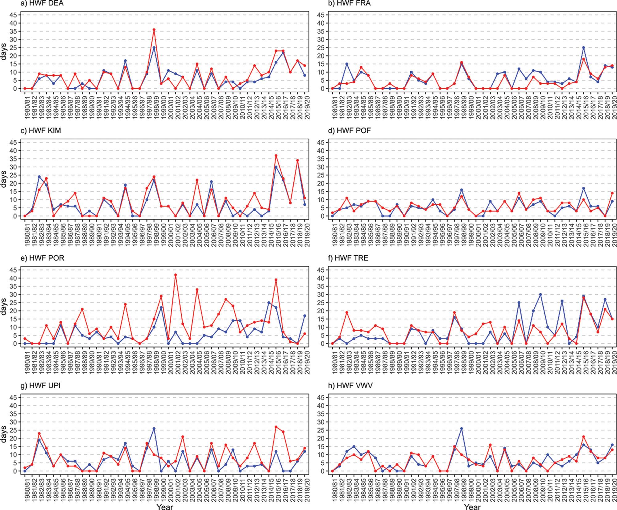
and 0.80 (KIM; Table 2). KIM shows the highest MD values for HWF (0.80) and HWN (0.80), but the lowest value for HWM (0.51; Table 2). The consistency observed in the moderate to strong MD values reflects a high degree of temporal consistency between the data sets (Table 2). Relatively low deviation across the data sets is also evident from the RMSE values, which are relatively low for all heatwave aspects (Table 2); despite this, these RMSE values are higher than that for Tms (Tables 1–2). The RMSE values provide support for the consistency and general deviation observed in the box plots (Supplementary figure 3; Table 2). Specifically, the HWF values range from 2.80 (POF) to 10.92 (POR) days, while HWM ranges from 1.34 (TRE) to 6.45 (POR) °C2, and HWN ranges from 0.71 (POF) to 2.40 (POR) events (Supplementary figure 3; Table 2). A larger degree of deviation exists between the stations and corresponding AgERA5 for HWF, and a smaller degree of deviation is evident for HWN (Table 2). Overall, the AgERA5 data set typically overestimates HWF and HWN, and consistent with the Tms biases, it typically underestimates HWM (Tables 1–2). For HWF, biases range between -1.33 (POR) and 5.60 days (FRA), while for HWM biases range from -1.55 (POR) to 1.47 °C2 (KIM), and for HWN the range is between -0.28 (POR) and 1.40 events (FRA; Table 2). This pattern in the biases is also evident in the time series plots and box plots (Figures 3–5; Supplementary figure 3).
AgERA5 representation of mean winter coldwave characteristics
Box plots and time series plots for coldwave characteristics of the weather stations and AgERA5 grid cells in the Northern Cape from 1980
to 2020, demonstrate a high degree of agreement between the data sets, albeit to a lesser extent than for Tmw (Supplementary figure 4; Figures 2a, 3–5). Strong agreement for the coldwave aspects is evidenced by typically overlapping boxes in the box plots and comparable temporal variability in the time series (Supplementary figure 4; Figures 6–8). However, for some locations (e.g. POR), the box plots show less overlap and less temporal agreement in the time series plots (Supplementary figure 4; Figures 6–8). Specifically, the box plots indicate that most locations deviate, on average, by <2 days for CWF, <2 °C2 for CWM and <0.5 events for CWN (Supplementary figure 4).
The mostly moderate to strong CC values (>0.5) for coldwave characteristics provide additional support for the conclusions drawn from the box plots and time series plots (Supplementary figure 4; Figures 6–8; Table 2). Lower CC values for CWM show that CWM was characterised by the weakest performance and CWM is the only index that has CC values that are statistically insignificant (Table 2). Specifically, for CWF, CC values range from 0.45 (POR) to 0.92 (DEA), for CWM, CC values range from 0.17 (POR) to 0.80 (UPI), and for CWN, the range is between 0.47 (POR) and 0.89 (DEA; Table 2). CC values generally suggest that the AgERA5 and SAWS data sets agree the most for CWF compared to CWM and CWN (Table 2). Additionally, the MD values demonstrate a similar pattern where the CWM aspect depicts the weakest performance (Table 2). For both the CC and MD values, weaker agreement for CWF and CWN is evident at KIM, POR, and TRE, whereas, for CWM, KIM has higher MD and CC values, and FRA has lower MD values compared to KIM for CWF and CWN (Table 2). More specifically, the MD values for CWF range from 0.40 (POR) to 0.80 (DEA), for CWM, values range from
Volume 120| Number 3/4 March/April 2024 69 https://doi.org/10.17159/sajs.2024/16043 Research Article Evaluation of AgERA5 temperature data across the Northern Cape Page 5 of 13
Figure 3: Time series plots depicting the total number of days contributing to annual summer heatwave events (HWF) for the AgERA5 (red) and SAWS (blue) data sets from 1980 to 2020 for locations mapped in Figure 1.
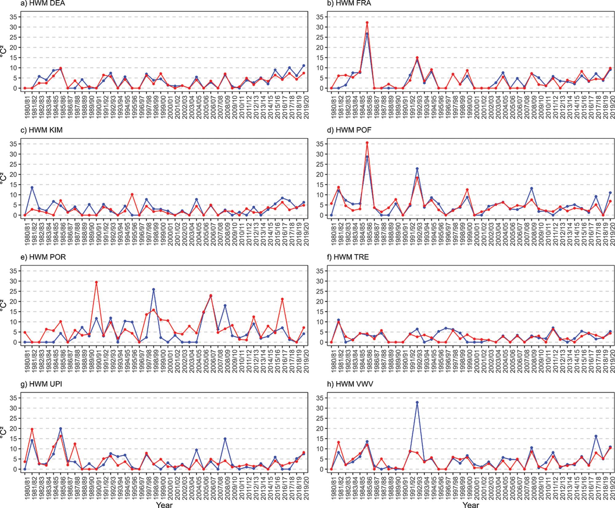
0.35 (POR) to 0.68 (POR), and for CWN, values range from 0.48 (POR) to 0.84 (DEA; Table 2). Deviation between coldwave characteristics, as inferred from the AgERA5 and SAWS data sets’ RMSE values, generally tends to be highest for CWF and lowest for CWN (Table 2). Regarding CWF, the RMSE values range from 3.25 (DEA) to 8.09 (POR) days, whereas for CWM, the range is from 2.32 (VWV) to 5.26 (KIM) °C2, and for CWN, values range from 0.73 (DEA) to 1.52 (POR) events (Table 2). Box plots in Supplementary figure 4, patterns observed in the time series plots (Figures 6–8), and the positive bias values in Table 2 suggest that the AgERA5 data set overestimates coldwave characteristics to a greater extent than Tmw (Tables 1–2); positive biases for CWM are consistent with that for Tmw (Tables 1–2). Specifically, the biases for CWF range from -1.61 (FRA) to 3.39 days (POR), for CWM the range is from -2.05 (FRA) to 2.91 (KIM) °C2, and for CWN the range is between -0.39 (FRA) and 0.71 (POR) events (Table 2). Bias values for POR and TRE are highest and lowest, respectively, for CWN and CWF, while the highest and lowest values for CWM are shown by POR and FRA, respectively (Table 2). This pattern is also apparent in the values calculated for CC and MD (Table 2).
Discussion and conclusions
Through a comparative analysis between weather stations and corresponding AgERA5 grid cells, we evaluated the accuracy of the AgERA5 representation of seasonal average and extreme temperature characteristics over the Northern Cape for 1980–2020. This study builds on research by Roffe and van der Walt20 by evaluating the
AgERA5 data set’s ability to represent Tms and Tmw, and the respective seasonal heatwave and coldwave characteristics, against point-based SAWS station data, as opposed to such evaluations using a gridded observation data set. This approach is advantageous as fewer biases are introduced into the evaluation as the point-based weather station data used herein has not been interpolated.20,44 We do, however, acknowledge that the station-based temperature data are not completely without biases due to, for instance, missing data and the methods used for estimation thereof, changes in station location and monitoring instrumentation, and land use/cover.44 Despite the weather station data limitations, their use for evaluation provides a robust understanding of the AgERA5 performance over the Northern Cape. Thus, the insights gained from this comparative analysis highlight limitations and advantages of using the AgERA5 product over the Northern Cape; these are important to consider for future research applying this data set to the Northern Cape.
The results presented herein reveal that the AgERA5 data set performs quite well over the Northern Cape, and is thus an invaluable data set to apply for future temperature-related research over the region. Over this data sparse region, the AgERA5 data set can be used, for instance, to analyse ETE impacts for areas with no existing weather station infrastructure.45 This would be particularly valuable to understand the temperature patterns over Kakamas (a town without a weather station) for instance, where, in January 2023, anomalously hot temperatures caused seven fatalities.46 This is not the only example in which ETEs have caused fatalities in South African regions where there are no weather
Volume 120| Number 3/4 March/April 2024 70 https://doi.org/10.17159/sajs.2024/16043 Research Article Evaluation of AgERA5 temperature data across the Northern Cape Page 6 of 13
Figure 4: Time series plots depicting the average temperature of annual summer heatwave events (HWM) for the AgERA5 (red) and SAWS (blue) data sets from 1980 to 2020 for locations mapped in Figure 1.
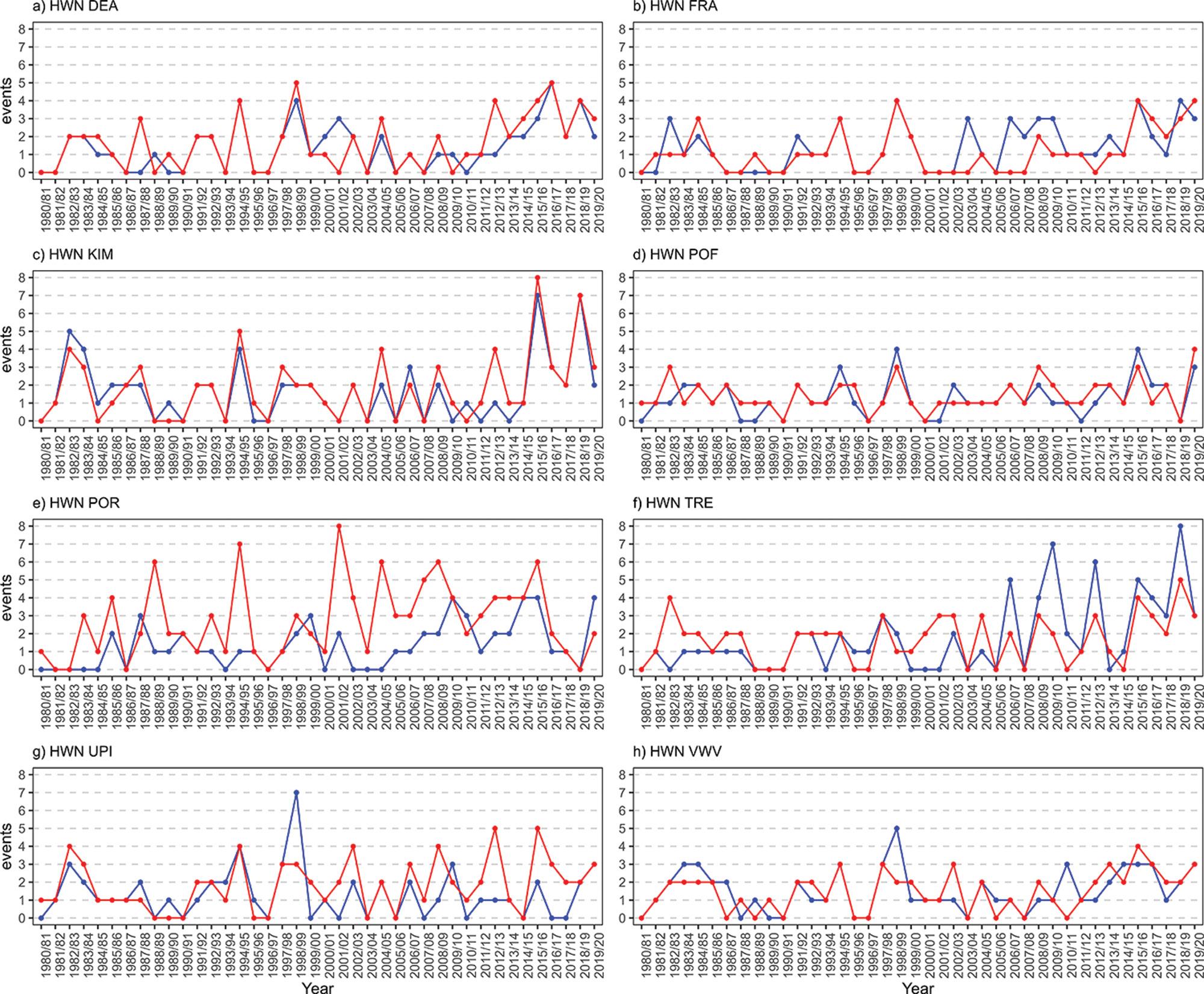
1980 to
between the AgERA5 and SAWS data sets for the total number of days contributing to annual summer (winter) heatwave (coldwave) events (HWF [CWF]), the average temperature of annual summer (winter) heatwave (coldwave) events (HWM [CWM]), and the total number of summer (winter) heatwave (coldwave) events (HWN [CWN]). CC represents the Spearman Correlation Coefficient; RMSE represents the Root Mean Square Error; MD represents the Modified Index of Agreement. CC values denoted in bold represent statistically significant correlations at the 5% alpha level.
...table 2 continues on next page
Volume 120| Number 3/4 March/April 2024 71 https://doi.org/10.17159/sajs.2024/16043 Research Article Evaluation of AgERA5 temperature data across the Northern Cape Page 7 of 13
IndexStationCCMDrMSEBias HWF DEA 0.80 0.764.041.28 FRA 0.72 0.753.84-1.33 KIM 0.87 0.804.401.53 POF 0.78 0.692.800.50 POR 0.66 0.4710.925.60 TRE 0.60 0.646.960.10 UPI 0.65 0.606.762.18 VWV 0.78 0.694.26-0.33
Figure 5: Time series plots depicting the total number of summer heatwave events (HWN) for the AgERA5 (red) and SAWS (blue) data sets from
2020 for locations mapped in Figure 1.
table 2: Tabulated results, per location mapped in Figure 1, of the comparison
Volume 120| Number 3/4 March/April 2024 72 https://doi.org/10.17159/sajs.2024/16043 Research Article Evaluation of AgERA5 temperature data across the Northern Cape Page 8 of 13 IndexStationCCMDrMSEBias HWM DEA 0.74 0.631.85-0.74 FRA 0.79 0.772.170.37 KIM 0.68 0.512.90-1.55 POF 0.73 0.762.61-0.51 POR 0.53 0.546.541.47 TRE 0.69 0.721.34-0.41 UPI 0.66 0.643.69-0.51 VWV 0.93 0.705.13-1.19 HWN DEA 0.74 0.780.990.23 FRA 0.68 0.741.01-0.28 KIM 0.85 0.800.870.20 POF 0.74 0.700.710.15 POR 0.53 0.442.401.40 TRE 0.56 0.591.64-0.10 UPI 0.60 0.581.480.50 VWV 0.68 0.691.00-0.05 CWF DEA 0.92 0.803.250.83 FRA 0.73 0.694.43-1.61 KIM 0.71 0.595.640.88 POF 0.78 0.743.781.10 POR 0.45 0.408.093.39 TRE 0.59 0.626.59-0.34 UPI 0.90 0.773.451.41 VWV 0.82 0.743.460.15 CWM DEA 0.52 0.583.280.02 FRA 0.250.363.67-2.05 KIM 0.57 0.565.262.91 POF 0.76 0.682.050.23 POR0.170.353.080.74 TRE 0.52 0.573.85-0.59 UPI 0.80 0.652.730.71 VWV 0.75 0.642.32-0.45 CWN DEA 0.89 0.840.73-0.10 FRA 0.70 0.711.08-0.39 KIM 0.62 0.571.310.10 POF 0.78 0.760.910.20 POR 0.47 0.481.520.71 TRE 0.53 0.631.47-0.17 UPI 0.85 0.760.810.17 VWV 0.66 0.641.050.12 table 2 continued...
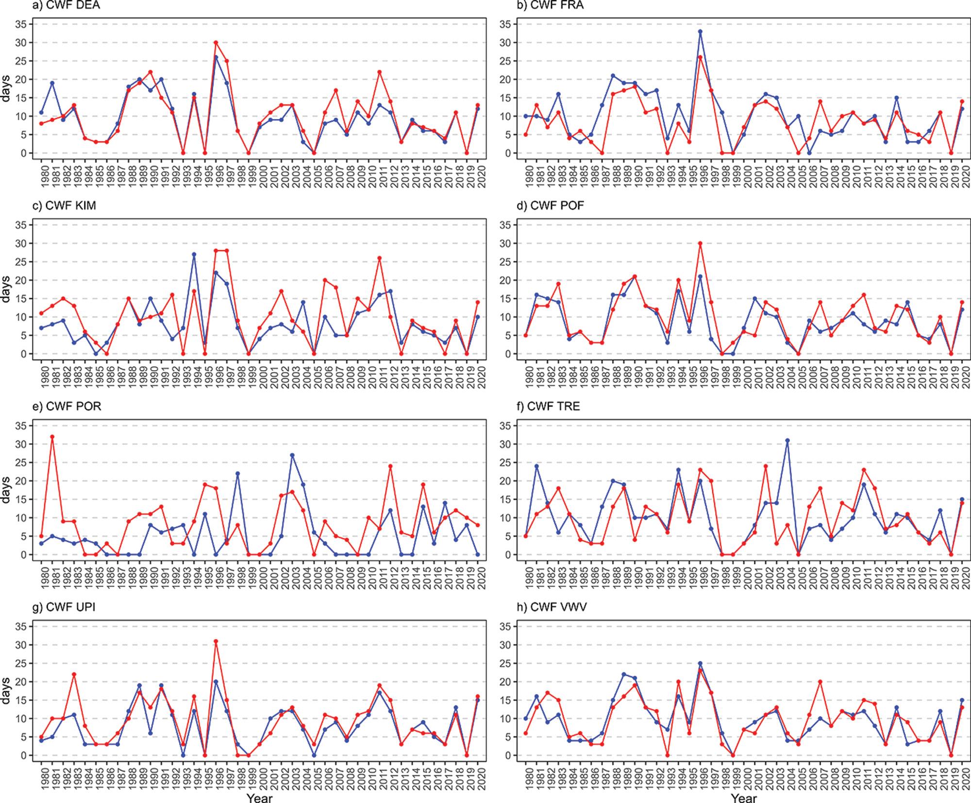
stations47; this highlights the value of a reliable gridded data set like the AgERA5. Moreover, by analysing ETEs with the AgERA5 data set, one can derive valuable information that can aid in developing efficient and prompt adaptive measures and strategies, which can aid in mitigating the negative impacts of ETEs, such as preventing heat stress, optimising crop management techniques, and enhancing infrastructure.7-9,48
In terms of the AgERA5 performance over the Northern Cape, general findings suggest strong, but varying, correspondence spatially, which is a result that is in agreement with the findings of similar studies.20-21 Mean seasonal temperatures correspond and perform better than heatwave and coldwave characteristics from AgERA5 (Tables 1–2). This is likely due to differences at the temperature distribution extremes between the station and AgERA5 data sets (Figure 2). Furthermore, a common limitation in statistical comparisons, known as the double penalty problem, of fine-resolution data based on point-to-point analysis also contributes to the weaker performance detected for the ETE characteristics.49 For instance, a temperature proxy may be penalised for a spurious observation due to imprecise station location, while an ETE proxy will be doubly penalised for issuing a false alarm for an ETE.49 Based on daily to annual temperature averages, it is evident that Tms performs slightly better than Tmw (Table 1). Across the stations, Tms is characterised by higher CC and MD values, indicating better correlation and agreement between predicted and observed values (Table 1). The present analysis demonstrates a predominant underestimation of Tms and Tmw by the AgERA5 temperature proxies (Table 1), which is a finding that corresponds to results presented by
Roffe and van der Walt20 and Velikou et al.21 Observed negative bias values between station and AgERA5 Tms and Tmw proxies can be considered a plausible explanation for the underestimation of HWM and CWM in the AgERA5 data set (Tables 1–2).20 Among the heatwave and coldwave indices, HWM and CWM represent the ETE characteristics with the poorest performance (Table 2), and this is a finding that aligns with previous research.20,21,29 While the AgERA5 data set performed well in representing heatwave and coldwave characteristics, these results highlight the need for caution when utilising the AgERA5 data set to examine HWM and CWM over the Northern Cape. The suboptimal performance of HWM and CWM therefore suggests that there is much room for improvement in the AgERA5 data set representation of temperatures at the tail ends of the temperature distribution. In contrast to HWM and CWM, HWF, HWN, CWF, and CWN exhibit positive biases relative to station data and demonstrate CC and MD values of greater magnitude (Table 2). While performance variations exist among different locations, and the difference in the performance of summer and winter ETE indices is relatively small, mean CC and MD values indicate superior performance for summer ETE indices compared to winter ETE indices (Tables 1–2). Stronger performance in summer ETE indices has also been observed in other studies.20
Although the overall performance was strong, some locations (i.e. POR, located along the western coast, and TRE, located in the Kalahari Desert) were consistently characterised by poorer performance (Tables 1–2), likely because these regions contain fewer stations compared to other parts of the Northern Cape.20 Moreover, mean and extreme temperatures
Volume 120| Number 3/4 March/April 2024 73 https://doi.org/10.17159/sajs.2024/16043 Research Article Evaluation of AgERA5 temperature data across the Northern Cape Page 9 of 13
Figure 6: Time series plots depicting the total number of days contributing to annual winter coldwave events (CWF) for the AgERA5 (red) and SAWS (blue) data sets from 1980 to 2020 for locations mapped in Figure 1.
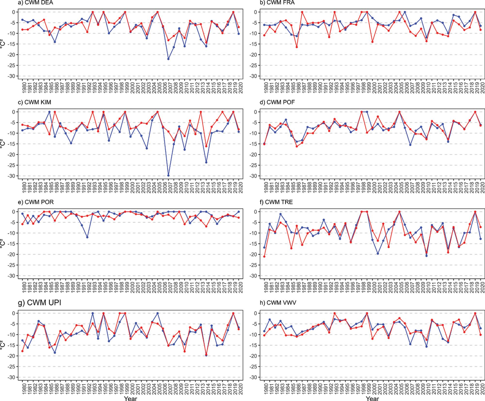
at locations bordering the Atlantic Ocean are strongly influenced by the cold Benguela Current (and Upwelling System) which proves to be a phenomenon that is not accurately simulated by the ECMWF modelling system.20,50 For TRE, in the Kalahari Desert region, the desert surface influences mean and extreme temperatures through cloud development mechanisms, which could also lead to parameterisation difficulties in the ERA5 reanalysis methods.16,50 Grid cells bordering the cold Benguela current or falling within the Kalahari Desert regions should be treated with caution, and limitations and uncertainties should be appropriately acknowledged. A better understanding of these weaknesses is critical for improving future parameterisation methods for the underlying ECMWF model used for the ERA5 reanalysis; this will undoubtedly lead to better accuracy for calculated indices and long-term trends. Despite the weaknesses identified herein, this ERA5 reanalysis product has shown strong improvement based on its predecessor (ERA-Interim) and will likely improve still in the foreseeable future.50 Furthermore, according to previous research comparing the AgERA5 data set to others, like AgCFSR and CPC, the AgERA5 outperforms these in terms of accuracy and reliability.51,52
The strengths and limitations of the AgERA5 presented herein support further application of the AgERA5 data set for characterising average and extreme temperatures over the Northern Cape. Findings suggest, based on moderate to strong CC values, that AgERA5 can effectively capture interannual variability patterns in the Northern Cape, and in turn will likely provide reliable trend results despite conflicting thoughts regarding the
application of reanalysis for trend calculations.20 This underscores the potential of AgERA5 as a valuable tool for studying long-term changes in the Northern Cape climate. Progressing forward, it would be important to utilise the ERA5 reanalysis to investigate synoptic-scale circulation patterns associated with the occurrence of coldwaves and heatwaves across the Northern Cape. Comprehending this using numerical weather prediction models can play an important role in the predictability of these events, ultimately informing better early warnings of ETEs over the Northern Cape.53
Acknowledgements
A.J.v.d.W. acknowledges the Emerging Scholar Research Programme of the University of the Free State and financial support from the Society of South African Geographers (SSAG) Centenary Award.
A.J.v.d.W., J.A.K. and S.J.R. acknowledge financial support from the Faculty of the Natural and Agricultural Sciences and the Geography Department of the University of the Free State. We also acknowledge the European Centre for Medium-Range Weather Forecasts (ECMWF) for the publicly available AgERA5 data used in this study, which is available from the Copernicus Climate Change Service website (https://cds.climate.copernicus.eu/cdsapp#!/dataset/10.24381/cds.6 c68c9bb?tab=overview).
Competing interests
We have no competing interests to declare.
Volume 120| Number 3/4 March/April 2024 74 https://doi.org/10.17159/sajs.2024/16043 Research Article Evaluation of AgERA5 temperature data across the Northern Cape Page 10 of 13
Figure 7: Time series plots depicting the average temperature of annual winter coldwave events (CWM) for the AgERA5 (red) and SAWS (blue) data sets from 1980 to 2020 for locations mapped in Figure 1.
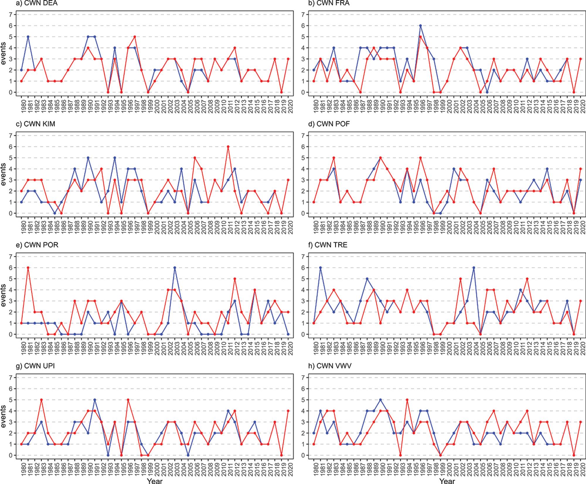
Authors’ contributions
J.A.K.: Conceptualisation, methodology, data collection, data analysis, datacuration,studentprojectmanagement,validation,writing–initialdraft. S.J.R.: Conceptualisation, methodology, data collection, data analysis, data curation, student project management, validation, writing – revisions, student supervision. A.J.v.d.W.: Conceptualisation, methodology, student project management, validation, writing – revisions, student supervision.
references
1. Mbokodo I, Bopape MJ, Chikoore H, Engelbrecht F, Nethengwe N. Heatwaves in the future warmer climate of South Africa. Atmosphere. 2020;11(7), Art. #712. https://doi.org/10.3390/atmos11070712
2. Engelbrecht F, Adegoke J, Bopape MJ, Naidoo M, Garl R, Thatcher M, et al. Projections of rapidly rising surface temperatures over Africa under low mitigation. Environ Res Lett. 2015;10(8), Art. #085004. https://doi.org/10.1 088/1748-9326/10/8/085004
3. Engelbrecht FA, Monteiro P. The IPCC assessment report six working group 1 report and southern Africa: Reasons to take action. S Afr J Sci. 2021;117 (11–12), Art. #12679. https://doi.org/10.17159/sajs.2021/12679
4. Van der Walt AJ, Fitchett JM. Exploring extreme warm temperature trends in South Africa: 1960–2016. Theor Appl Climatol. 2021;143:1341–1360. https ://doi.org/10.1007/s00704-020-03479-8
5. Iyakaremye V, Zeng G, Zhang G. Changes in extreme temperature events over Africa under 1.5 and 2.0 °C global warming scenarios. Int J Climatol. 2021;41(2):1506–1524. https://doi.org/10.1002/joc.6868
6. Van der Walt AJ, Fitchett JM. Trend analysis of cold extremes in South Africa: 1960–2016. Int J Climatol. 2021;41(3):2060–2081. https://doi.org/10.100 2/joc.6947
7. Campbell S, Remenyi TA, White CJ, Johnston FH. Heatwave and health impact research: A global review. Health Place. 2018;53:210–218. https:// doi.org/10.1016/j.healthplace.2018.08.017
8. Lobell DB, Bänziger M, Magorokosho C, Vivek B. Nonlinear heat effects on African maize as evidenced by historical yield trials. Nat Clim Change. 2011;1:42–45. https://doi.org/10.1038/nclimate1043
9. Nienaber JA, Hahn GL. Livestock production system management responses to thermal challenges. Int J Biometeorol. 2007;52:149–157. https://doi.org/1 0.1007/s00484-007-0103-x
10. Abatan AA, Abiodun BJ, Lawalc KA, Gutowski WJ. Trends in extreme temperature over Nigeria from percentile-based threshold indices. Int J Climatol. 2015;36(6):2527–2540. https://doi.org/10.1002/joc.4510
11. Harrington J, Otto F. Reconciling theory with the reality of African heatwaves. Nat Clim Chang. 2020;10:796–798. https://doi.org/10.1038/s41558-020-0 851-8
Volume 120| Number 3/4 March/April 2024 75 https://doi.org/10.17159/sajs.2024/16043 Research Article Evaluation of AgERA5 temperature data across the Northern Cape Page 11 of 13
Figure 8: Time series plot representing the total number of winter coldwave events (CWN) for the AgERA5 (red) and SAWS (blue) data sets from 1980 to 2020 for all locations mapped in Figure 1.
12. Tyson PD, Preston-Whyte RA. The atmosphere and weather of southern Africa. 2nd ed. Cape Town: Oxford University Press; 2000. https://catalog.ha thitrust.org/api/volumes/oclc/42309991.html
13. Jury MR, Parker B. Cold winters over the South African highveld: Pattern recognition and preliminary models. S Afr J Sci. 1999;94:473–481. https://h dl.handle.net/10520/AJA00382353_239
14. Levey KM. Interannual temperature variability and associated synoptic climatology at Cape Town. Int J Clim. 1996;16(3):293–306. https://doi.org/1 0.1002/(SICI)1097-0088(199603)16: 3%3C293::AID-JOC3%3E3.0.CO;2-3
15. Driver P, Reason CJC. Variability in the Botswana High and its relationships with rainfall and temperature characteristics over southern Africa. Int J Climatol. 2017;37(S1):570–581. https://doi.org/10.1002/joc.5022
16. Manatsa D, Reason C. ENSO–Kalahari Desert linkages on southern Africa summer surface air temperature variability. Int J Climatol. 2017;37(4):1728–1745. https://doi.org/10.1002/joc.4806
17. Mbokodo IL. Heat waves in South Africa: Observed variabilty, structure and trends [master’s dissertation]. Thohoyandou: University of Venda; 2017.
18. Mkiva N. The Climatology of heat waves in the North West Province, South Africa [master’s dissertation]. Potchefstroom: North-West University; 2020.
19. Van der Walt AJ, Fitchett JM. Extreme Temperature Events (ETEs) in South Africa: a review. S Afr Geogr J. 2021;104(1):70–88. https://doi.org/10.1080 /03736245.2021.1907219
20. Roffe SJ, Van der Walt AJ. Representation and evaluation of southern Africa’s seasonal mean and extreme temperatures in the ERA5-based reanalysis products. Atmos Res. 2023;284(106591):0169-8095. https://doi.org/10.1 016/j.atmosres.2022.106591
21. Velikou K, Lazoglou G, Tolika K, Anagnostopoulou C. Reliability of the ERA5 in replicating mean and extreme temperatures across Europe. Water. 2022;14(4):543. https://doi.org/10.3390/w14040543
22. Schumacher V, Justino F, Fernández A, Meseguer‐Ruiz O, Sarricolea P, Comin A. Comparison between observations and gridded data sets over complex terrain in the Chilean Andes: Precipitation and temperature. Int J Climatol. 2020;40(12):5266–5288. https://doi.org/10.1002/joc.6518
23. Harris I, Osborn TJ, Jones P, Lister D. Version 4 of the CRU TS monthly highresolution gridded multivariate climate dataset. Sci Data. 2020;7:109. https:/ /doi.org/10.1038/s41597-020-0453-3
24. Gelaro R, McCarty W, Suárez MJ, Todling R, Molod A, Takacs L, et al. The modern-era retrospective analysis for research and applications, version 2 (MERRA-2). J Clim. 2017:30(14):5419–5454. https://doi.org/10.1175/JCL I-D-16-0758.1
25. Hersbach H, Bell B, Berrisford P, Hirahara S, Horányi A, Muñoz‐Sabater J, et al. The ERA5 global reanalysis. Q J R Meteorol Soc. 2020;146(730):1999–2049. https://doi.org/10.1002/qj.3803
26. C3S. Copernicus climate change service climate data store [data set on the Internet]. c2020 [cited 2022 Mar 29]. https://doi.org/10.24381/cds.6c68c 9bb
27. Oyler JW, Dobrowski SZ, Ballantyne AP, Klene AE, Running SW. Artificial amplification of warming trends across the mountains of the western United States. Geophys Res Lett. 2015;42(1):153–161. https://doi.org/10.1002/2 014GL062803
28. Roffe SJ, Fitchett JM, Curtis CJ. Quantifying rainfall seasonality across South Africa on the basis of the relationship between rainfall and temperature. Clim Dyn. 2021;56:2431–2450. https://doi.org/10.1007/s00382-020-05597-5
29. KellerJD,WahlS.Representationofclimateinreanalyses:Anintercomparison for Europe and North America. J Clim. 2021;34(5):1667–1684. https://doi.o rg/10.1175/JCLI-D-20-0609.1
30. Schulzweida U. CDO user guide. Hamburg: Max Planck Institute for Meteorology; 2021 [cited 2023 Apr 14]. Available from: https://code.mpimet .mpg.de/projects/cdo/embedded/index.html
31. Herold N, McComb J. Climpact [software on the Internet]. GitHub; 2021. [cited 2022 Sep 07]. Available from: https://github.com/ARCCSS-extremes /climpact
32. VanderWaltAJ,FitchettJM.StatisticalclassificationofSouthAfricanseasonal divisions on the basis of daily temperature data. S Afr J Sci. 2020;116 (9–10), Art. #7614. https://dx.doi.org/10.17158/sajs.2020/7614
33. Kruger AC, Nxumalo M. Surface temperature trends from homogenized time series in South Africa: 1931–2015. Int J Climatol. 2017;37(5):2364–2377. https://doi.org/10.1002/joc.4851
34. Klein Tank AMG, Zwiers FW, Zhang X. Guidelines on analysis of extremes in a changing climate in support of informed decisions for adaptation. Geneva: World Meteorological Organization; 2009.
35. Durre I, Menne MJ, Gleason BE, Houston TG, Vose RS. Comprehensive automated quality assurance of daily surface observations. J Appl Meteorol Climatol. 2010;49(8):1615–1633. https://doi.org/10.1175/2010JAMC2375.1
36. Lakhraj‐Govender R, Grab S, Ndebele NE. A homogenized long‐term temperature record for the Western Cape Province in South Africa: 1916–2013. Int J Climatol. 2016;37(5):2337–2353. https://doi.org/10.1002/joc.4 849
37. Wolski P, Conradie S, Jack C, Tadross M. Spatio‐temporal patterns of rainfall trends and the 2015–2017 drought over the winter rainfall region of South Africa. Int J Climatol. 2021;41(S1):E1303–E1319. https://doi.org/10.1002/ joc.6768
38. Perkins SE, Alexander L V. On the measurement of heat waves. J Clim. 2013;26(13):4500–4517. https://doi.org/10.1175/JCLI-D-12-00383.1
39. Nairn JR, Fawcett RJ. The excess heat factor: a metric for heatwave intensity and its use in classifying heatwave severity. Int J Environ Res Public Health. 2014;12(1):227–253. https://doi.org/10.3390/ijerph120100227
40. Perkins-Kirkpatrick SE, Gibson PB. Changes in regional heatwave characteristics as a function of increasing global temperature. Sci Rep. 2017;7, Art. #12256. https://doi.org/10.1038/s41598-017-12520-2
41. Wang C, Zhang L, Lee SK, Wu L, Mechoso CR. A global perspective on CMIP5 climate model biases. Nat Clim Change. 2014;4:201–205. https://doi.org/1 0.1038/nclimate2118
42. Li CZ, Zhang L, Wang H, Zhang YQ, Yu FL, Yan DH. The transferability of hydrological models under nonstationary climatic conditions. Hydrol Earth Syst Sci. 2012;16(4):1239–1254. https://doi.org/10.5194/hess-16-1239-2 012
43. Willmott CJ, Matsuura K. Advantages of the mean absolute error (MAE) over the root mean square error (RMSE) in assessing average model performance. Clim Res. 2005;30:79–82. https://doi.org/10.3354/cr030079
44. Sheridan SC, Lee CC, Smith ET. A comparison between station observations and reanalysis data in the identification of extreme temperature events. Geophys Res Lett. 2020;47(15), Art. #2020GL088120. https://doi.org/10. 1029/2020GL088120
45. Van der Walt AJ, Kruger JA, Roffe SJ. Fine-resolution analysis of the spatiotemporalcharacteristicsofheatwavesintheMaloti-Drakensbergregion, southern Africa: 1979–2021. Trans R Soc South Africa. 2023;78(1/2):5–15. https://doi.org/10.1080/0035919X.2023.2175075
46. Khumalo Z. Heat wave claims lives of 5 people in Northern Cape. News24. 2023 January 20. Available from: https://www.sajs.co.za/vancouver-refere ncing-style
47. CRED. The international disaster database, EM-DAT query tool [database on the Internet]. c2023 [cited 2023 Sep 24]. Available from: https://www.emd at.be/
48. Stöllberger C, Lutz W, Finsterer J. Heat‐related side‐effects of neurological and non‐neurological medication may increase heatwave fatalities. Eur J Neurol 2009;16(7):879–882. https://doi.org/10.1111/j.1468-1331.2009.0 2581.x
49. Dee DP, Uppala SM, Simmons AJ, Berrisford P, Poli P, Kobayashi, et al. The ERA-Interim reanalysis: Configuration and performance of the data assimilation system. Q J R Meteorol Soc. 2011;137(656):553–597. https: //doi.org/10.1002/qj.828
Volume 120| Number 3/4 March/April 2024 76 https://doi.org/10.17159/sajs.2024/16043 Research Article Evaluation of AgERA5 temperature data across the Northern Cape Page 12 of 13
50. Gleixner S, Demissie T, Diro GT. Did ERA5 improve temperature and precipitation reanalysis over East Africa? Atmosphere. 2020;11(9):996. htt ps://doi.org/10.3390/atmos11090996
51. Araghi A, Martinez CJ, Olesen JE, Hoogenboom G. Assessment of nine gridded temperature data for modeling of wheat production systems. Comput Electron Agric. 2022;199, Art. #107189. https://doi.org/10.1016/j.compag .2022.107189
Evaluation
52. Lagos-Zúñiga M, Balmaceda-Huarte R, Regoto P, Torrez L, Olmo M, Lyra A, et al. Extreme indices of temperature and precipitation in South America: Trends and intercomparison of regional climate models. Clim Dyn. 2022. https://doi .org/10.1007/s00382-022-06598-2
53. Bobape M-JM, Sebego E, Ndarana T, Maseko B, Netshilema M, Gijben M, et al. Evaluating South African Weather Service information on Idai tropical cyclone and KwaZulu-Natal flood events. S Afr J Sci. 2021;117(3–4), Art. #7911. https://dx.doi.org/10.17159/sajs.2021/7911
Volume 120| Number 3/4 March/April 2024 77 https://doi.org/10.17159/sajs.2024/16043 Research Article
Page 13 of 13
of AgERA5 temperature data across the Northern Cape
AuthorS:
Maxine J. Turner1
Sandy van Vuuren1
Stephanie Leigh-de Rapper1
AFFILIAtIoN:
1Department of Pharmacy and Pharmacology, University of the Witwatersrand, Johannesburg, South Africa
CorrESPoNDENCE to:
Stephanie Leigh-de Rapper
EMAIL:
stephanie.derapper@wits.ac.za
DAtES:
received: 09 Jun. 2023
revised: 17 Nov. 2023
Accepted: 26 Jan. 2024
Published: 27 Mar. 2024
hoW to CItE:
Turner MJ, van Vuuren S, Leigh-de Rapper S. Analysing patient factors and treatment impact on diabetic foot ulcers in South Africa. S Afr J Sci. 2024;120(3/4), Art. #16301. https:// doi.org/10.17159/sajs.2024/16301
ArtICLE INCLuDES:
☒ Peer review
☒ Supplementary material
DAtA AVAILABILItY:
☐ Open data set
☐ All data included
☒ On request from author(s)
☐ Not available
☐ Not applicable
EDItorS:
Pascal Bessong
Shane Redelinghuys
KEYWorDS:
diabetic foot, polypharmacy, chronic disease, prevention and control
FuNDING:
South African National Research Foundation; University of the Witwatersrand
Analysing patient factors and treatment impact on diabetic foot ulcers in South Africa
In the South African public healthcare sector, 28% of diabetic patients present to primary healthcare clinics with diabetic foot ulcers (DFUs), often presenting in advanced stages of ulcer severity. In this study, we aimed to categorise factors predisposing individuals to developing a DFU and to identify the potential shortcomings in existing treatment plans in the South African healthcare system. In addition, the use of preventative measures in the management of DFUs was examined as well as the influence of past treatment practices. A total minimum sample size of 50 DFUs was required for this study. Participants who were selected for this study had their past records reviewed in order to determine the likelihood of previous DFU infections, as well as to determine the occurrence of co-morbidities. The treatment protocol implemented was recorded. Twelve-month patient records were used to identify the infection frequency and past treatment protocols. A total of 48.9% of patients reported that they did not make use of any preventative measures. The most frequent concurrent medical conditions were hypertension, dyslipidaemia, and peripheral neuropathy. Polypharmacy was prevalent, with 55% of the population prescribed five or more medications. Potential medication interactions were examined and a total of 210 interactions were documented. An analysis of past and current treatment practices revealed that 52.1% of the treatment protocols did not comply with local treatment guidelines. This study highlights the urgent need for updated DFU treatment protocols in relation to the overall management of DFUs, taking into account existing international guidelines.
Significance:
We determined that the South African treatment guidelines and DFU classification system do not align to international standards. Furthermore, the use of preventative measures among DFU patients was poor and polypharmacy was present in the patient cohort. We emphasise the need for all members of a healthcare team, including podiatrists, clinicians, microbiologists and pharmacists, to work together in order to identify at-risk patients, prevent possible DFUs and effectively treat existing DFUs in a manner that does not contribute to antimicrobial resistance and provides the best possible outcome for the patient.
Introduction
Diabetic foot syndrome, a complication of diabetes mellitus, is the most common cause of hospitalisation and lower limb amputation among diabetic patients.1 A foot ulcer is defined as a full-thickness wound below the ankle on a weight-bearing or exposed surface that involves at least the epidermis layer and part of the dermis layer of the skin.2,3 By definition, a diabetic foot ulcer (DFU) is a foot ulcer in a person with diagnosed diabetes mellitus and typically presents alongside neuropathy or peripheral artery disease in the lower extremity.3 Neuropathic DFUs often result in the formation of open wounds, the primary risk factor for the development of infections of the DFU.4 It is estimated that over 50% of DFUs become infected, which increases the risk of amputation and mortality.4
South Africa is trying to move towards universal health coverage; however, at the time of this study, provision of health care in South Africa consisted of an unequal two-tiered system. The first is the public sector, which is state funded and services the majority of the population, and the second is the private sector, which is funded mostly by individual contributions to medical aid schemes or health insurance.5 This study focused on patients within the public healthcare system. In the South African province of KwaZulu-Natal, there are approximately 1.4 million diabetic patients who access public health care, with approximately 2400 amputations performed annually.6 A five-year audit of the amputations that occurred in one KwaZulu-Natal hospital found that 53.1% of amputations were due to diabetes mellitus.7 A more recent study in KwaZulu-Natal determined that 53.7% of amputations were attributable to diabetes mellitus.8 The high rate of amputation in KwaZulu-Natal corresponds to the findings of another study undertaken in 2018 whereby patients presented to rural healthcare facilities with advanced stages of DFU severity, requiring amputations as a result.9 A study undertaken in the Gauteng province of South Africa ascertained that 1565 DFU-related amputations occurred over a period of 30 months.10 These findings highlight the seriousness of the consequences of DFUs and the need to reduce their prevalence and improve treatment protocols.
Knowledge and practice regarding DFUs, as well as the ability to identify individuals at risk of developing a DFU, are vital in reducing complications and subsequent lower limb amputation. Thus, an understanding of the treatment of DFUs in the South African public healthcare sector by all healthcare professionals is necessary in order to improve patient outcomes through improved treatment guidelines. The aim of this study was to categorise factors that predispose individuals to develop a DFU and to identify the potential shortcomings in existing treatment plans. In addition, the use of preventative measures and past treatment practices in the management of DFUs was examined.
78 https://doi.org/10.17159/sajs.2024/16301 Volume 120| Number 3/4 March/April 2024 © 2024. The Author(s). Published under a Creative Commons Attribution Licence.
Research Article
Methods
Ethical considerations and setting
Ethical clearance was obtained from the Human Research Ethics Committee (HREC) of the University of the Witwatersrand (M210431) and study site approval was obtained from two tertiary public healthcare institutions in Johannesburg, South Africa. The study design chosen was an observational cross-sectional study with retrospective analysis. Patient confidentiality was maintained through the use of key numbers which were ascribed to all participants (for example, A001, A002). The patient information leaflet was given to the patient before they gave informed consent to participate in the study. In addition, consent was garnered from all participants for the capture and use of photographs relating to the patient’s DFU wound. The principal investigator of this study, unless otherwise stated, was responsible for capturing all photographic evidence. The research project was registered with the South African National Health Research Database (GP_202108_026).
A total of 45 patients with 50 DFUs were recruited for this study, thus meeting the expected sample size for this cohort. This sample size was calculated based on a 95% confidence interval and a 50% drop-out rate. The decreased prevalence of DFUs in this setting due to the COVID-19 pandemic was considered in the sample size calculation. Participation was on the day of study enrolment and no follow-up visits were required.
Patient selection and classification
All patients attending the study site’s podiatry and wound clinics were selected and invited to participate in this study. Subjects identified to participate had to be diagnosed as diabetic and present with a DFU. Paediatric patients were excluded from participation in this study. Patient selection was based on purposive, homogeneous sampling as the goal of this research is to understand the influence of patient-specific factors on DFU development and subsequent treatment plans.
Patients were classified as having type 1 or type 2 diabetes based on the patient’s history obtained from the file review or interview. Once classified by diabetic type, patients were further classified by level of DFU infection. This classification is dependent on the severity of the ulcer and is mild, moderate or severe as per the South African Antimicrobial Stewardship guidelines (Table 1).11 The patient’s DFU was subsequently classified according to the Wagner classification (Table 1) in order to
compare the most commonly used classification system worldwide to the South African guidelines on DFU classification.
Patient record review and administration of a structured questionnaire
Participants who were selected for this study had their past records reviewed in order to determine the likelihood of previous DFU infections as well as to determine the occurrence of co-morbidities. The treatment protocol implemented was recorded alongside the number of infections treated and if sample cultures were taken. Twelve-month patient records were used to identify the infection frequency, the causative micro-organism (if identified) and the antimicrobial used to treat the DFU. This information assisted in determining the prevalence of DFU and the prescribing patterns of antimicrobials, which guided the development of the treatment policy. A short, structured questionnaire was used in order to determine the use of preventative aids that had been prescribed, or had not been prescribed but were independently initiated by participants. The structured questionnaire contained a section on demographic information in order to establish if certain patients were more likely to present with DFUs. Next, a section on concurrent conditions and chronic medication use was included in order to establish the effect of these factors on ulcer severity. A section on preventative measure use was included in order to establish both the frequency of their use and patient compliance. Rather than using a self-administered questionnaire, the patients were interviewed in order to overcome any language or understanding barriers.
Validating the retrospective review tool
The retrospective review tool was adapted from a South African study which looked at resistance patterns in urinary tract infections.13 Validation of the retrospective review tool, in order to ensure its reliability in the context of its use, was completed by means of a pilot study. Two patients from the Charlotte Maxeke Johannesburg Academic Hospital podiatry unit were randomly selected. This site was used as it had been approved by both the hospital and ethics committee.
The two patients who participated in the pilot study comprise an acceptable sample size as the established sample size for the study was limited. The two patients proved the reliability of the retrospective review tool by answering all the questions without needing assistance or further explanation. Conducting the pilot study led to the addition of different preventative measures that were not previously included, for example, a walker. These changes were approved by the HREC prior to the commencement of the study.
results
the Wagner classification system
GradeLesion
0No open lesions; deformity or cellulitis may be present
1Superficial ulcer; partial or full thickness
2 Ulcer extension to ligament, tendon, joint capsule, or deep fascia without abscess or osteomyelitis
3Deep ulcer with abscess, osteomyelitis, or joint sepsis
4Gangrene localised to portion of forefoot or heel
5Extensive gangrenous involvement of the entire foot
the South African antimicrobial stewardship classification system
ClassificationDescription
Mild Limited to skin/superficial subcutaneous tissue <2 cm beyond ulcer margin
Moderate Cellulitis >2 cm, deep fascial involvement, gangrene, abscess, osteomyelitis
SevereSystemic complications
Patient demographics
An understanding of patient demographics is required for all members of a healthcare team in order to identify at-risk patients timeously. Nonmodifiable factors like age and gender play a role in the development of DFUs.14,15 The results from this study demonstrate a higher prevalence of DFU among male participants (60%) in comparison to female participants (40%). Table 2 depicts the age groups of participants in the study. The oldest participant was 80 years old, while the youngest was 36 years old. The median age of participants was 59 (n=45).
The use of classification systems in the treatment of DFUs
A patient-specific comparison of ulcer classification, with photographic reference to each ulcer, is provided in Supplementary table 1. In this study, the majority of patients presented with Wagner grade 1 DFUs (33.3%) and Wagner grade 2 DFUs (33.3%). Wagner grade 3 ulcers were seen in 17.6% of patients while Wagner grade 4 ulcers were seen in 13.7% of patients. Only one patient presented with a Wagner grade 5 ulcer. When comparing the South African classification system to the Wagner classification system, it is noted that the systems are very different in relation to detail and diagnosis. For example, the South African Antimicrobial Stewardship Programme (SAASP) ‘mild’ classification includes DFUs from Wagner grades 1, 2 and 3. This suggests that the Wagner classification system is more descriptive than the SAASP
Volume 120| Number 3/4 March/April 2024 79 https://doi.org/10.17159/sajs.2024/16301 Research Article Treating diabetic foot ulcers in South Africa Page 2 of 9
table 1: The Wagner and South African Antimicrobial Stewardship classification systems4,11,12
30–40
41–50
51–60
>
Total
guidelines and allows for more selective categorisation of different ulcers based on their severity. As a result, 60.8% of participants presented with mild ulcers (Wagner grades 1, 2 and 3), 37.3% with moderate ulcers (Wagner grades 2, 3 and 4) and 1.9% with severe ulcers (Wagner grade 4) according to SAASP guidelines.
The presence of co-morbidities and complications
Understanding the influence that co-morbidities have on the pathogenesis of DFUs is important as it enables healthcare professionals to screen, prevent or treat in a manner that does not worsen or promote DFU formation. Hypertension was found to be present in 84.4% of patients –making it the most common concurrent medical condition amongst this cohort. Table 3 provides a summary of the co-morbidities identified in the patient cohort.
In this study, 93.3% of patients presented with at least one chronic condition in addition to diabetes mellitus, 80% presented with at least two concurrent chronic conditions, and 40% presented with more than four co-morbidities. The highest number of concurrent conditions reported was eight; while the most frequently seen number of concurrent chronic conditions was two. The average number of co-morbidities in addition to diabetes mellitus seen in this patient cohort was 3.9 ≈ 4.
Patients who exhibited either Wagner grade 1 or 4 ulcers presented with the highest average number of chronic co-morbid conditions. The largest proportion of ulcers were classified as grade 1 or grade 2 in severity, and these patients presented with an average number of 4.1 and 3.8 co-morbidities, respectively.
Medication use and the incidence of polypharmacy
Diabetic patients are twice as likely as non-diabetic patients to experience a drug-drug interaction due to the presence of multiple co-morbid conditions in the diabetic population.16 The most commonly used medication was found to be metformin (850 mg) taken either twice or three times daily. In total, 68.9% of patients were taking metformin. Insulin was used by 62.2% of patients, with the most frequently used form being actraphane, a biphasic human insulin. Of the medications that are not anti-diabetic in nature, the most frequently used include simvastatin (for hyperlipidaemia treatment), enalapril and amlodipine (both used in the treatment of hypertension), with 40% of patients found to be using these medications. Thereafter, the use of hydrochlorothiazide (a diuretic used in the treatment of hypertension) and paracetamol (an analgesic and antipyretic) was the next most frequently noted (33.3%). Table 4 summarises the total number of medications taken per patient, per day.
In this study’s sample population, 44.4% of patients were found to be prescribed between one and five medications. Within this group, 15.5% of patients were prescribed two medications, making it the most frequently used number of medications. Thereafter, 11.1% of patients were found to be prescribed either seven or nine chronic medications. The highest number of medications used by a single patient was 14 and the lowest was 1. The majority of the sample population (55.5%) were noted to be prescribed more than five medications.
A total of 210 potential drug-drug interactions were observed in the patient cohort. The most frequently seen type of interaction in this study was moderate drug interactions (55.2%). The mean number of drug interactions per patient was 4.7. Only 35.6% of participants in this study did not present with any potential drug-drug interactions, while 60% and
table 3: Co-morbidity prevalence
Concurrent condition
heart failure, atrial fibrillation, angina and dilated cardiomyopathy)
Number of patients presenting with the condition
Average Wagner score of patients presenting with the concurrent condition
Eczema2 (4.4)2
Visual impairment2 (4.4)1
Gastro-oesophageal
Myasthenia gravis1 (2.2)2
Chronic kidney stones1 (2.2)3
Venous insufficiency1 (2.2)3
Rheumatoid arthritis1 (2.2)1
Iron deficiency anaemia1 (2.2)2
table 4: The number of different medications taken daily by the patient cohort
Number of medicationsFrequency of patients (%)
1–520 (44.4)
6–1020 (44.4)
>105 (11.1)
57.8% of patients presented with moderate or severe interactions. The largest number of potential drug interactions seen per patient was 21. This number of interactions was seen in one patient and the same patient was noted to be on the highest number of medications (n=14). The average number of medications used in patients presenting with both Wagner grades 1 and 2 DFUs was six (Table 5). The highest average number of medications used (n=7) was seen in those with DFUs of Wagner grade 3 severity.
Non-pharmacological management: Preventative measures and pressure offloading devices
The prevention of DFUs should be the primary goal of all healthcare practitioners treating diabetic patients. It is at this stage that educating
Volume 120| Number 3/4 March/April 2024 80 https://doi.org/10.17159/sajs.2024/16301 Research Article Treating diabetic foot ulcers in South Africa Page 3 of 9
AgeNumber of participantsPercentage
years24
years613
years1840
60 years1942
number of patients45100
table 2: The age groups of participants in this study
(%)
Hypertension38 (84.4) 2.4 ≈ 2 Dyslipidaemia15 (33.3) 2.1 ≈ 2 Peripheral neuropathy12 (26.7) 2.2 ≈ 2
8 (17.8) 2.8 ≈ 3 Metabolic syndrome5 (11.1) 2.6 ≈ 3 Gout3 (6.7) 2.7 ≈ 3 Hypothyroidism3 (6.7)4 Renal disease3 (6.7)2 Asthma2 (4.4) 2.5 ≈ 3
obstructive pulmonary disorder 2
Cardiovascular disease (including
Chronic
(4.4)2
Depression / generalised anxiety disorder 2 (4.4) 2.5 ≈ 3
reflux disorder / peptic ulcers 2 (4.4)1
the patient on preventative measures is important and can be done by all healthcare professionals. In this study, 48.9% of patients did not make use of any preventative measures. The frequency and type of preventative measures used by patients in the study cohort are given in Figure 1.
The results regarding the use of preventative measures were used to determine if there was a correlation between the use of these interventions and ulcer severity. Table 6 compares the severity of the DFU, according to the Wagner classification, to the use of preventative measures.
From Table 6, it can be seen that the most commonly used method of pressure off-loading for all grades of ulcer severity is crutches, which were used by 32.4% of patients overall. Except for those patients with DFUs classified as Wagner grade 2, the average number of preventative measures used is less than one for all grades of ulcer severity. The only instance in which crutches are not the most frequently used off-loading measure is in those patients with Wagner grade 3 ulcers. In those instances, removable walkers are more frequently used.
Pharmacological management and treatment practices
By evaluating the past treatment plan of patients in this cohort, gaps and missed opportunities in past treatment practices could be identified. This allows for the improvement of DFU treatment plans in the future. Table 7 describes the treatment protocols observed in the study population and compares the treatment practices observed to both local and international guidelines. South African guidelines suggest oral antimicrobial therapy of amoxicillin/clavulanic acid, flucloxacillin and clindamycin in the case of penicillin allergy. Due to missing files, and new patients with no file history, seven patients (15.6%) did not have comprehensive records of treatment protocols for previous or current
DFUs. From the information available from the remaining 38 patient files, 48 treatment protocols were recorded. Of these, 47.9% complied with those set out in the South African guidelines. Only 14.6% of treatment protocols were partially compliant, 33.3% were not compliant and the remaining 4.2% of the protocols could not be assessed for compliance due to a lack of record keeping or because of treatment of unrelated foot conditions (onychomycosis). While the majority of patients were treated in a manner that adhered to the local guidelines, the repeated treatment
table 6: Comparison between ulcer severity and preventative measure use
1
walker (25%); walker (16.7%); wheelchair (16.7%)
2 Crutches (41.2%); wheelchair (29.4%)
3
4
walker (28.6%); walker, wheelchair, crutches, specialised footwear (14.3% each)
(60%);
walker (20%); wheelchair (20%)
5
Volume 120| Number 3/4 March/April 2024 81 https://doi.org/10.17159/sajs.2024/16301 Research Article Treating diabetic foot ulcers in South Africa Page 4 of 9
Wagner classification Number of patients Average number of medications Average number of interactions 11764 21764 3975 4765 5174
system 0 5 10 15 20 25 No preventative measures used CrutchesWheelchairRemovable walker Walker "Off the counter" footwear Prescribed footwear Num be r o f pa ti en ts
table 5: The average number of medications and potential interactions observed as classified by the Wagner classification
Figure 1: The use of preventative measures.
Number of DFu patients Average number of preventative methods
patient Number of patients not
Wagner grade Most frequent preventative measure used
used per
using preventative measures
Removable
120.77
161.15
90.86
Removable
Crutches
removable
70.63
101
No preventative measures used
Volume 120| Number 3/4 March/April 2024 82 https://doi.org/10.17159/sajs.2024/16301 Research Article Treating diabetic foot ulcers in South Africa Page 5 of 9 Patient code Date of current and previous treatments Wagner grade at most recent date Antibiotic prescribed Alignment to the StG or SAASP Alignment to international guidelines Number of chronic medications prescribed A00121/04/20212 Yes CPC7 A00207/03/20212 Yes NCNC2 A003 12/03/20212NoNCNC 10 20/08/20211 Yes CPC A00420/08/20211 Yes CPC2 A00506/08/20212 Yes CPC9 A006 a 2 aaa 2 A007 01/04/2019 1 & 4 NoNCNC 6 02/09/2019 Yes NCNC 30/07/2021 Yes CPC A00823/08/20212 Yes CPC2 A00921/06/20213 & 1NoNCNC6 A010 17/02/2020 Yes CPC 12 11/08/20203 Yes CPC A01113/07/20212 Yes CPC8 A01203/06/20212 & 1 Yes PCPC4 A01313/09/20212NoNCNC5 A014 a 3 aaa 1 A01509/20212NoNCNC4 A016 a 3 aaa 9 A01707/12/20212 & 4 Yes CPC4 A01816/11/20213 & 1 Yes CPC1 A019 b 4 bbb 2 A02020/12/20212 Yes NCNC14 A021Feb-211NoNCNC2 A022 25/12/2021 - 31/12/2021 1 Yes UnknownUnknown5 A023 c 1 ccc 3 A024 c 1 ccc 7 A025 7/02/2022 1 Yes CPC 3 29/12/2020 Yes PCPC A026 b 1 bbb 7 A02703/03/20224 Yes PCPC14 A028 22/02/2022 2 Yes N/AN/A 7 24/03/2022 Yes PCPC A02908/03/20224 Yes NCC8 A03007/03/20224 Yes CPC5 A03107/03/20223 Yes CPC4
...table 7 continues on next page
table 7: Comparison of treatment protocols recorded in patient files to South African and international guidelines as well as to the incidence of polypharmacy
Key: STG, Standard Treatment Guidelines; SAASP, South African Antimicrobial Stewardship Programme; C, compliant; PC, partially compliant; NC, non-compliant
a patient file unaccounted for
b new patient, no file history
c new file created as previous file was lost due to a fire at Charlotte Maxeke Johannesburg Academic Hospital
plans observed, and the number of patients with chronic wounds, suggest that these guidelines do not cover the most commonly isolated pathogens.17 It was further found that 60.4% of the treatment protocols implemented complied only partially to international guidelines.
Discussion
In this study, the greatest rate of incidence of ulceration occurred in those over the age of 60 years (42%), while only 17% of DFUs were seen in patients younger than 50 years of age. These results are consistent with the findings of a systematic review and meta-analysis carried out in 2022, in which increasing age, and subsequent longer duration of diabetes, was found to be a consistent risk factor associated with DFU incidence and consequent lower limb amputation.18 According to a meta-analysis evaluating the influence of epidemiologic and patient behaviour related predictors on amputation rates in diabetic patients, the male sex was found to be a significant risk factor for amputation.19 A higher prevalence of DFUs among male patients in this study was consistent with previous studies carried out across India.1-3 The prevalence of DFUs has been suggested to be greater among the male population due to an increased incidence of peripheral neuropathy, a higher likelihood of exposure to trauma in comparison to female patients, as well as a greater tendency for female patients to carry out foot care regimens more frequently than male patients.18,20-22
Comparing the South African classification system to the Wagner classification system suggests that the Wagner classification system allows for more selective categorisation of different ulcers than the SAASP guidelines based on ulcer severity. As a result, patients presenting in the South African public healthcare sector with varying degrees of ulcer severity are treated in the same broad manner with very little difference in treatment between degrees of severity. The use of the SAASP guidelines in conjunction with the Standard Treatment Guidelines and Essential Drug List results in no difference in the treatment plans of Wagner grades 1 through 5 DFUs to account for increasing severity. It is thus important to consider changing the South African guidelines, to those which are more capable of discerning DFUs of different severity, and subsequent treatment plans, such as those provided for by the International Working Group on the Diabetic Foot (IWGDF).23
Many South African patients with diabetes are managed in primary healthcare clinics where healthcare providers are responsible for playing a role in the prevention of disease and education of patients.24 Should screening for diabetes-related complications not occur effectively, individuals presenting with these complications will be missed, resulting in delayed treatment, increased healthcare cost and poor patient outcomes.24 Patients in this study were expected to present on a monthly basis in order to monitor the progression of their DFU as well as track the management of diabetes and related co-morbidities. In this study, hypertension was found to be present in 84.4% of patients, making it
Volume 120| Number 3/4 March/April 2024 83 https://doi.org/10.17159/sajs.2024/16301 Research Article Treating diabetic foot ulcers in South Africa Page 6 of 9
Patient code Date of current and previous treatments Wagner grade at most recent date Antibiotic prescribed
StG
Alignment to the
or SAASP
A03207/03/20224NoNCNC6 13/03/20225 Yes NCC7 A033 A03409/03/20223 Yes CPC9 A03503/03/20222NoNCNC8 A03618/03/20222 Yes CPC3 A03713/03/20223 Yes CPC11 A038 26/02/2021 Yes CPC 10 12/03/20221 Yes PCC A039 09/02/2022 3 Yes CPC 8 21/03/2022 Yes CPC A04022/03/20221 Yes PCPC12 A04101/04/20222 Yes PCPC9 A042 16/07/2016 2 NoNCNC 9 10/06/2022NoNCNC A04310/06/20221NoNCNC2 A044 23/08/2021 1 Yes CPC 10 17/06/2022 Yes CPC A04521/06/20222 Yes CPC5
Alignment to international guidelines Number of chronic medications prescribed
table 7 continued...
the most common concurrent medical condition amongst this cohort. This result is consistent with another South African study in which it was found that 85.7% of DFU patients presented with hypertension.25
Hypertension is a critical co-morbidity in patients presenting with DFUs as it results in atrial wall stiffening and thus further promotes the advancement of peripheral artery disease and subsequent DFU development. The proportion of patients with hypertension in our study is greater than that of previous studies which had 58.3–69.9% of patients presenting with hypertension.24,26 This result is congruent with the World Health Organization’s findings that low- to middle-income countries have a higher incidence of hypertension amongst their population.27
Dyslipidaemia (total cholesterol: >5.2 mmol/L; LDL cholesterol: >2.6 mmol/L; HDL cholesterol: <1.6 mmol/L or triglycerides: >1.7 mmol/L) was reported in 33.3% of patients. A study undertaken in Egypt concluded that the presence of dyslipidaemia significantly increased the risk for DFU development.28 In contrast, a systematic review carried out in 2021 concluded that, while dyslipidaemia is often associated with type 2 diabetes mellitus, it is not associated with diabetic foot conditions.14 While conflicting reports exist about the relationship between dyslipidaemia and DFU risk, patients presenting with dyslipidaemia are 2.23 times more likely to develop peripheral neuropathy, a significant factor in the pathophysiology of DFUs.4,29
Upon review of the patient files, it was noted whether the patient had received a diagnosis of peripheral neuropathy as well as what treatment was prescribed, if any. The incidence of peripheral neuropathy, as documented in the patients’ files, was 46%. From the results obtained, an additional 29% of patients presented with signs and symptoms of peripheral neuropathy, but remained undiagnosed and untreated. Thus, the more likely incidence of peripheral neuropathy in the study population may be closer to 75%. This finding is corroborated by a study undertaken in Sudan, where it was reported that the incidence of peripheral neuropathy associated with DFU was 82.1%.30 In India, it was reported that 95.8% of DFU patients presented with peripheral neuropathy.31
An additional concern is that patients’ health conditions are not effectively reported in their files and that patient record keeping is not effectively implemented and monitored. This is problematic in that medical practitioners may miss critical information about previous diagnoses, treatments and prescriptions when assessing and providing new treatment plans for patients.32 A study undertaken in public healthcare centres in South Africa, which aimed to identify healthcare provider related determinants of diabetes and hypertension management, found that co-morbid conditions, as well as special investigations concerning the progression of disease, were infrequently noted.33 The lack of complete patient health records often results in poorer quality patient care, and further adversely effects clinical research.34
In order to reduce the need for antimicrobial use, and thus reduce the burden of disease and antimicrobial resistance, education on the prevention of diabetic foot ulcers is paramount.35,36 Preventative measures in this study were examined in order to determine whether the best treatment practices are employed in the South African public healthcare sector. It was established that 48.9% of patients did not make use of any preventative measures. Of patients who did make use of preventative measures, the most commonly used form of pressure off-loading was crutches (26.7%). A removable walker, which is one of the most effective preventative measures, was used by only 20% of patients.36,37 Specialised footwear, including footwear marketed in commercial stores for diabetic patients, was only observed in 6.7% of patients.
In the South African context, the Standard Treatment Guidelines call for the education of patients regarding foot care; however, according to a study undertaken in a regional hospital in Durban (KwaZulu-Natal, South Africa), 90% of diabetic patients had not received any education of diabetic foot disease.38,39 In addition to this, it was found that only 22.2% of DFU patients reported that they had personally examined their feet, and moreover, that these patients examined their feet only after developing a problem.38 This further indicates a lack of understanding arising from a dearth of education pertaining to the importance of foot
care in the diabetic patient. A similar study in Malaysia reported that 58% of patients did not have sufficient knowledge regarding foot care, and 61.8% of patients had poor foot care practices.40 A study undertaken in India found that general foot care practice was poor, with many patients found to walk barefoot. Furthermore, 67.7% of patients did not check their footwear for foreign objects before putting them on and 54.8% of patients did not participate in regular foot care activities such as cutting their toenails.41 A more recent study undertaken in Brazil found that 65.5% of participants had little knowledge regarding preventative measure use.42 In the South African healthcare context, patients initially present to a primary healthcare clinic. Healthcare professionals at primary healthcare clinics are responsible for the screening of diseases and referral to higher levels of health care should the need arise.43 It has been suggested that diabetic foot assessments and preventative measure implementation may be overlooked on account of the healthcare professionals stationed at these clinics being overworked and understaffed.43
When comparing use of preventative measures to ulcer severity, as a general trend, when ulcer severity increases, the likelihood of previous lower extremity amputation, as a result of a DFU, increases. This is concerning because patients who had undergone previous lower extremity amputation as a result of previous foot ulceration are presenting with DFUs with higher grades of severity. This infers that consequent patient education, or a lack thereof, as well as previous DFU experience of the patient, does not aid in the prevention of DFU reoccurrence and additional amputation. These findings were corroborated by a study undertaken in 14 European healthcare centres where a high ulcer reoccurrence rate was documented, despite regular follow-ups and continued patient education.44 The importance of effective patient education is thus emphasised, with various reviews highlighting its crucial role in preventing DFUs and reducing their social and economic burden to society.45,46
In this study, the majority of patients presented with grade 1 DFUs (33.3%) and grade 2 DFUs (33.3%). Grade 3 ulcers were seen in 17.6% of patients while grade 4 ulcers were seen in 13.7% of patients. Only one patient presented with a grade 5 ulcer. A study undertaken in Nigeria observed the most common ulcer severity as grade 4 (36.9%), followed by grade 3 (26.2%) and grade 2 (17%).47 Another study undertaken in India found the most common ulcer severity as grade 4 (34%), followed by grade 2 (22%) and grade 1 (18%).48 A possible explanation as to why fewer ulcers of higher severity were observed in this study is because patients were often admitted at casualty and transferred directly to surgical wards without any further consultation from other healthcare professionals like podiatrists. From there, many patients underwent amputations, and as such were excluded from the study. This possibility is concerning, as patients would not be given the opportunity to undergo less aggressive methods of treatment and be subjected to a poorer quality of life due to the loss of a limb. A study evaluating the management of DFUs found that half of DFU amputations can be prevented with proper treatment.49 Polypharmacy is most commonly defined as the use of five or more medications in a day.16 Patients presenting with type 2 diabetes, in particular older patients, are at risk for polypharmacy due to the nature of treating both macrovascular and microvascular complications of diabetes.16 It has been found that diabetic patients are twice as likely to experience a drug-drug interaction when compared to patients without diabetes due to the presence of multiple co-morbid conditions in the diabetic populations; it is therefore important to monitor patients’ prescriptions.16 A review looking at the prevalence of polypharmacy in older diabetic patients found that 64% of patients were prescribed more than four medications a day.50 In the current study, we found that 55.5% of the sample population were prescribed more than five medications on a chronic basis. This review also highlighted that polypharmacy may reduce optimal glycaemic control as well as increase the risk of hospitalisation.50
The average number of medications used by patients presenting with both grade 1 and 2 DFUs in this study was six. The highest average number of medications used (7) was seen in those with DFUs of Wagner grade 3 severity. In this study, the average number of drug-drug interactions was 4.7. It has been found that the presence of both polypharmacy and
Volume 120| Number 3/4 March/April 2024 84 https://doi.org/10.17159/sajs.2024/16301 Research Article Treating diabetic foot ulcers in South Africa Page 7 of 9
subsequent potential drug interactions may alter glycaemic targets and result in a deterioration in renal function.50 This not only poorly affects the overall health of the patient, but impaired renal function is also associated with delayed ulcer healing, amputation and mortality.50 It is therefore important to effectively manage patients who take multiple medications. This can be accomplished by reviewing the patient’s full medication history every time a new drug is considered, improving and increasing clinical pharmacy services, improving communication between healthcare practitioners, and, finally, by implementing effective patient history reporting and record-keeping.
Therefore, in conclusion, addressing the concerns relating to diabetes and DFU management identified in this study are crucial. Large-scale studies should be conducted to review the entire South African context for the magnitude of DFU incidence and management concerns, including adherence to treatment plans and the influence of DFU progression. These studies could help to address the development and implementation of more comprehensive patient education programmes to ensure that individuals with DFUs are well informed about the importance of complying with lifestyle changes and prescribed medications. In addition, these studies would aid in establishing robust monitoring and follow-up systems, which are required when tracking patient progress in adhering to treatment plans and reducing DFU burden.
Acknowledgements
This study was funded by the South African National Research Foundation Researcher Rating fund in addition to the University of the Witwatersrand Faculty of Health Sciences Research Committee fund.
Competing interests
We have no competing interests to declare.
Authors’ contributions
S.v.V.: Conception or design; acquisition, analysis, or interpretation of data; drafting the work or revising; and final approval of the manuscript. M.J.T.: Acquisition, analysis, or interpretation of data; drafting the work or revising; and final approval of the manuscript. S.L-d.R: Conception or design; acquisition, analysis, or interpretation of data; drafting the work or revising; and final approval of the manuscript.
references
1. McDermott K, Fang M, Boulton AJM, Selvin E, Hicks CW. Etiology, epidemiology, and disparities in the burden of diabetic foot ulcers. Diabetes Care. 2022;46:209–221. https://doi.org/10.2337/dci22-0043
2. Shin L, Armstrong D, Sanders LJ. Foot ulcers. In: Johns Hopkins Diabetes Guide [webpage on the Internet]. c2020 [cited 2023 Mar 29]. Available from:
3. Van Netten JJ, Bus SA, Apelqvist J, Lipsky BA, Hinchliffe RJ, Game F, et al. Definitions and criteria for diabetic foot disease. Diabetes Metab Res Rev. 2020;36, e3268. https://doi.org/10.1002/dmrr.3268
4. Chastain CA, Klopfenstein N, Serezani CH, Aronoff DM. A clinical review of diabetic foot infections. Clin Podiatr Med Surg. 2019;36:381–395. https://do i.org/10.1016/j.cpm.2019.02.004
5. Maphumulo WT, Bhengu BR. Challenges of quality improvement in the healthcare of South Africa post-apartheid: A critical review. Curationis. 2019;42(1):e1–e9. https://doi.org/10.4102/curationis.v42i1.1901
6. Naidoo U, Ennion L. Barriers and facilitators to utilisation of rehabilitation services amongst persons with lower-limb amputations in a rural community in South Africa. Prosthet Orthot Int. 2019;43:95–103. https://doi.org/10.117 7/0309364618789457
7. Manickum P, Ramklass SS, Madiba TE. A five-year audit of lower limb amputations below the knee and rehabilitation outcomes: The Durban experience. J Endocrinol Metab Diabetes S Afr. 2019;24:41–45. https://doi .org/10.1080/16089677.2018.1553378
8. Khan MZ, Smith MT, Bruce JL, Kong VY, Clarke DL. Evolving indications for lower limb amputations in South Africa offer opportunities for health system improvement. World J Surg. 2020;44:1436–1443. https://doi.org/10.1007/s 00268-019-05361-9
9. Cheddie S, Manneh C, Pillay B. Spectrum of disease and outcome of primary amputation for diabetic foot sepsis in rural KwaZulu-Natal. S Afr J Surg. 2018;56:16–19. https://doi.org/10.17159/2078-5151/2018/v56n3a2486
10. Ntuli SM, Letswalo DM. Diabetic foot amputations at central and provincial hospital in Gauteng. A signpost for inadequate foot health services at primary healthcare level in South Africa [preprint]. Research Square; version 1; 2011. https://doi.org/10.21203/rs.3.rs-955192/v1
11. WassermanS,BoylesT,MendelsonM.Apocketguidetoantibioticprescribing for adults in South Africa 2015: South African Antimicrobial Stewardship Programme; 2015.
12. Monteiro-Soares M, Boyko EJ, Jeffcoate W, Mills JL, Russell D, Morbach S, et al. Diabetic foot ulcer classifications: A critical review. Diabetes Metab Res Rev. 2020;36(Suppl 1), e3272. https://doi.org/10.1002/dmrr.3272
13. Jaji B. The antimicrobial resistance patterns of urinary tract infections (UTIs) in a South African public hospital [dissertation]. Johannesburg: University of the Witwatersrand; 2021.
14. Rossboth S, Lechleitner M, Oberaigner W. Risk factors for diabetic foot complications in type 2 diabetes – A systematic review. Endocrinol Diabetes Metab. 2020;4, e00175-e. https://doi.org/10.1002/edm2.175
15. Di Giovanni P, Scampoli P, Meo F, Cedrone F, D’Addezio M, Di Martino G, et al. The impact of gender on diabetes-related lower extremity amputations: An Italian regional analysis on trends and predictors. Foot Ankle Surg. 2021;27:25–29. https://doi.org/10.1016/j.fas.2020.01.005
16. Dobrică E-C, Găman M-A, Cozma M-A, Bratu OG, Pantea Stoian A, Diaconu CC. Polypharmacy in type 2 diabetes mellitus: Insights from an internal medicine department. Medicina. 2019;55:436. https://doi.org/10.3390/me dicina55080436
17. Turner M. Antimicrobial susceptibility patterns in diabetic foot ulcers in South African public hospitals [dissertation]. Johannesburg: University of the Witwatersrand; 2022.
18. Rodrigues BT, Vangaveti VN, Urkude R, Biros E, Malabu UH. Prevalence and risk factors of lower limb amputations in patients with diabetic foot ulcers: A systematic review and meta-analysis. Diabetes Metab Syndr: Clin Res Rev. 2022;16, Art. #102397. https://doi.org/10.1016/j.dsx.2022.102397
19. Shin JY, Roh S-G, Lee N-H, Yang K-M. Influence of epidemiologic and patient behavior-relatedpredictorsonamputationratesindiabeticpatients:Systematic review and meta-analysis. Int J Low Extrem Wounds. 2017;16:14–22. https: //doi.org/10.1177/1534734617699318
20. Kateel R, Augustine AJ, Prabhu S, Ullal S, Pai M, Adhikari P. Clinical and microbiological profile of diabetic foot ulcer patients in a tertiary care hospital. Diabetes Metab Syndr: Clin Res Rev. 2018;12:27–30. https://doi.org/10.10 16/j.dsx.2017.08.008
21. Krishnamurthy SR. Risk factor analysis in diabetic foot ulcer patients. IOSRJDMS. 2018;17:10–13. https://doi.org/10.9790/0853-1704161013
22. Sorber R, Abularrage CJ. Diabetic foot ulcers: Epidemiology and the role of multidisciplinary care teams. Semin Vasc Surg. 2021;34:47–53. https://doi. org/10.1053/j.semvascsurg.2021.02.006
23. Lipsky BA, Senneville É, Abbas ZG, Aragón-Sánchez J, Diggle M, Embil JM, etal.Guidelinesonthediagnosisandtreatmentoffootinfectioninpersonswith diabetes (IWGDF 2019 update). Diabetes Metab Res Rev. 2020;36, e3280. https://doi.org/10.1002/dmrr.3280
24. Owolabi EO, Goon DT, Ajayi AI, Adeniyi OV, Chu KM. Coverage of diabetes complications screening in rural Eastern Cape, South Africa: A crosssectional survey. S Afr Fam Pract. 2022;64:e1–e6. https://doi.org/10.4102 /safp.v64i1.5447
25. Dikeukwu RA, Omole OB. Awareness and practices of foot self-care in patients with diabetes at Dr Yusuf Dadoo district hospital, Johannesburg. J Endocrinol Metab Diabetes S Afr. 2013;18:112–118. https://doi.org/10.1080 /22201009.2013.10872314
26. AbdulghaniHM,AlRajehAS,AlSalmanBH,AlTurkiLS,AlNajashiNS,IrshadM, et al. Prevalence of diabetic comorbidities and knowledge and practices of foot care among diabetic patients: A cross-sectional study. Diabetes Metab Syndr Obes. 2018;11:417–425. https://doi.org/10.2147/dmso.s171526
27. World Health Organization. Hypertension [Internet]. 2022 [cited 2022 Jul 27]. Available from: https://www.who.int/news-room/fact-sheets/detail/hypertens ion
Volume 120| Number 3/4 March/April 2024 85 https://doi.org/10.17159/sajs.2024/16301 Research Article Treating diabetic foot ulcers in South Africa Page 8 of 9
28. AbdAllah AM, Sharafeddin M. Lipid profile disorders and diabetic foot risk; Is there a relationship between them? Zagazig Univ Med J. 2022;28:217–225. https://doi.org/10.21608/zumj.2020.25230.1765
29. Khawaja N, Abu-Shennar J, Saleh M, Dahbour SS, Khader YS, Ajlouni KM. The prevalence and risk factors of peripheral neuropathy among patients with type 2 diabetes mellitus; the case of Jordan. Diabetol Metab Syndr. 2018;10, Art. #8. https://doi.org/10.1186/s13098-018-0309-6
30. Almobarak AO, Awadalla H, Osman M, Ahmed MH. Prevalence of diabetic foot ulceration and associated risk factors: An old and still major public health problem in Khartoum, Sudan? Ann Transl Med. 2017;5:340–347. https://doi .org/10.21037/atm.2017.07.01
31. Sharma R, Kapila R, Sharma AK, Mann J. Diabetic foot disease – Incidence and risk factors: A clinical study. J Foot Ankle Surg. 2016;3:41–46. https://d oi.org/10.5005/jp-journals-10040-1046
32. Marutha N, Ngoepe M. The role of medical records in the provision of public healthcare services in the Limpopo province of South Africa. Afr J Inf Manag. 2017;19:1–8. https://doi.org/10.4102/sajim.v19i1.873
33. Steyn K, Levitt NS, Patel M, Fourie J, Gwebushe N, Lombard C, et al. Hypertension and diabetes: Poor care for patients at community health centres. S Afr Med J. 2008;98:618–622. https://doi.org/10.1080/2220100 9.2008.10872172
34. Odekunle FF, Odekunle RO, Shankar S. Why sub-Saharan Africa lags in electronic health record adoption and possible strategies to increase its adoption in this region. Int J Health Sci. 2017;11:59–64.
35. Abbas Z. The diabetic foot worldwide: Sub‐Saharan Africa. Foot Diabetes. 2020:51–60. https://doi.org/10.1002/9781119445821.ch4c
36. Schaper NC, van Netten JJ, Apelqvist J, Bus SA, Hinchliffe RJ, Lipsky BA. Practical guidelines on the prevention and management of diabetic foot disease (IWGDF 2019 update). Diabetes Metab Res Rev. 2020;36(Suppl 1), e3266. https://doi.org/10.1002/dmrr.3266
37. Wu SC, Jensen JL, Weber AK, Robinson DE, Armstrong DG. Use of pressure offloading devices in diabetic foot ulcers: Do we practice what we preach? Diabetes Care. 2008;31:2118–2119. https://doi.org/10.2337/dc08-0771
38. Goie TT, Naidoo M. Awareness of diabetic foot disease amongst patients with type 2 diabetes mellitus attending the chronic outpatients department at a regional hospital in Durban, South Africa. Afr J Prim Health Care Fam Med. 2016;8:e1–e8. https://doi.org/10.4102/phcfm.v8i1.1170
39. South African Department of Health. Primary healthcare standard treatment guideline and essential medicine list. 7th ed. Pretoria: National Department of Health Essential Drug Programme; 2020.
40. Muhammad-Lutfi AR, Zaraihah MR, Anuar-Ramdhan IM. Knowledge and practice of diabetic foot care in an in-patient setting at a tertiary medical center. Malays Orthop J. 2014;8:22–26. https://doi.org/10.5704/moj.1411 .005
41. Selvakumar S, Shah PB. Awareness and practice regarding foot self-care among patients of known type 2 diabetes mellitus in a rural area. Int J Community Med Public Health. 2017;3:861–864. https://doi.org/10.18203 /2394-6040.ijcmph20160917
42. Sousa VM, Sousa IA, Moura KR, Lacerda LSA, Ramos MGS, da Silva ARV. Knowledge about preventive measures for the development of diabetic foot. Rev Rene. 2020;21, e42638. https://doi.org/10.15253/2175-6783.202021 42638
43. Ntuli S, Swart A, Lambert CV. Risk factors for diabetic foot ulceration. S Afr J Diabetes Vasc Dis. 2018;15:32–36.
44. Dubský M, Jirkovská A, Bem R, Fejfarová V, Skibová J, Schaper NC, et al. Risk factors for recurrence of diabetic foot ulcers: Prospective follow-up analysis in the Eurodiale subgroup. Int Wound J. 2013;10:555–561. https://doi.org/1 0.1111/j.1742-481x.2012.01022.x
45. Ibrahim A. Diabetic foot ulcer: Synopsis of the epidemiology and pathophysiology. Int J Diabetes Endocrinol. 2018;3:23. https://doi.org/10.1 1648/j.ijde.20180302.11
46. Rigato M, Pizzol D, Tiago A, Putoto G, Avogaro A, Fadini GP. Characteristics, prevalence, and outcomes of diabetic foot ulcers in Africa. A systemic review and meta-analysis. Diabetes Res Clin Pract. 2018;142:63–73. https://doi.org /10.1016/j.diabres.2018.05.016
47. Ugwu E, Adeleye O, Gezawa I, Okpe I, Enamino M, Ezeani I. Burden of diabetic foot ulcer in Nigeria: Current evidence from the multicenter evaluation of diabetic foot ulcer in Nigeria. World J Diabetes. 2019;10:200–211. https://do i.org/10.4239/wjd.v10.i3.200
48. Mehraj M. A review of Wagner classification and current concepts in management of diabetic foot. Int J Orthop Sci. 2018;4:933–935. https://doi. org/10.22271/ortho.2018.v4.i1n.133
49. Weledji EP, Fokam P. Treatment of the diabetic foot – to amputate or not? BMC Surg. 2014;14:83. https://doi.org/10.1186/1471-2482-14-83
50. Remelli F, Ceresini MG, Trevisan C, Noale M, Volpato S. Prevalence and impact of polypharmacy in older patients with type 2 diabetes. Aging Clin Exp Res. 2022;34:1969–1983. https://doi.org/10.1007/s40520-022-02165-1
Volume 120| Number 3/4 March/April 2024 86 https://doi.org/10.17159/sajs.2024/16301 Research Article Treating diabetic foot ulcers in South Africa Page 9 of 9
AuthorS:
Manisha du Plessis1
Carla Fourie1
Heloise le Roux1
Anna-Mart Engelbrecht1,2
AFFILIAtIoNS:
1Department of Physiological Sciences, Faculty of Science, Stellenbosch University, Stellenbosch, South Africa
2African Cancer Institute (ACI), Department of Global Health, Faculty of Medicine and Health Sciences, Stellenbosch University, Cape Town, South Africa
CorrESPoNDENCE to:
Manisha du Plessis
EMAIL:
manishadup@sun.ac.za
DAtES:
received: 03 Oct. 2022
revised: 08 Nov. 2023
Accepted: 13 Nov. 2023
Published: 27 Mar. 2024
hoW to CItE:
du Plessis M, Fourie C, le Roux H, Engelbrecht A-M. Sanguinarine highly sensitises breast cancer cells to doxorubicin-induced apoptosis. S Afr J Sci. 2024;120(3/4), Art. #14917. https://doi.org/10.17159/sajs.202 4/14917
ArtICLE INCLuDES:
☒ Peer review
☒ Supplementary material
DAtA AVAILABILItY:
☐ Open data set
☐ All data included
☐ On request from author(s)
☒ Not available
☐ Not applicable
EDItorS:
Pascal Bessong
Shane Redelinghuys
KEYWorDS:
breast cancer, MKP-1, doxorubicin, MAPKs, autophagy, apoptosis
FuNDING:
South African National Research Foundation (118566), Cancer Association of South Africa, South African Medical Research Council
Sanguinarine highly sensitises breast cancer cells to doxorubicin-induced apoptosis
Breast cancer is the most commonly diagnosed cancer and the second most common cause of cancer death in women. The anthracycline, doxorubicin, is a well-known and highly effective treatment for breast cancer patients; however, many patients present with resistance to chemotherapeutic drugs, which ultimately results in treatment failure and contributes to high mortality rates. It is well established that the mitogen-activated protein kinase phosphatase 1 (MKP-1) mediates the response to chemotherapy, where upregulated MKP-1 is associated with chemoresistance. We investigated whether MKP-1 inhibition or silencing can sensitise triple-negative MDA-MB-231 breast cancer cells to doxorubicin therapy. We found that MKP-1 inhibition and silencing sensitises breast cancer cells to doxorubicin-induced apoptosis. Additionally, the inhibition of MKP-1 in combination with doxorubicin treatment promotes autophagy induction, while doxorubicin and not MKP-1 modulation increased lysosomal acidic compartments. As such, this study demonstrated that MKP-1 inhibition has a potential therapeutic benefit for breast cancer patients by increasing the efficacy of conventional chemotherapy. Therefore, MKP-1 inhibition should be developed as a clinically relevant adjuvant therapy, which could provide a novel avenue for therapeutic intervention in combination with chemotherapy in breast cancer patients.
Significance:
• MKP-1 inhibition with sanguinarine and silencing sensitises breast cancer cells to doxorubicin-induced apoptosis.
• The inhibition of MKP-1 with sanguinarine in combination with doxorubicin treatment promotes autophagy induction.
• MKP-1 inhibition can have a potential therapeutic benefit for breast cancer patients by increasing the efficacy of conventional chemotherapy.
Introduction
Currently, 90% of chemotherapy failures are related to drug resistance.1 Resistance to cytotoxic chemotherapeutic agents may often be random and unpredictable and becomes apparent only at clinical assessment.2 One such chemotherapeutic agent is the anthracycline, doxorubicin (Dox), which is often used as a first-line therapy for the treatment of breast cancer.3-5 However, its clinical effects are limited due to its dose-dependent side effects such as cardiotoxicity, gastrointestinal problems, acute vomiting, liver damage and nephropathy.6,7 Therefore, adjuvant therapies are required that can improve the effectiveness of Dox while conferring a protective effect on normal cells.
The mitogen-activated protein kinase phosphatase 1 (MKP-1) is a member of the MKP family that consists of 11 dual-specificity phosphatases that negatively regulate MAPK. Upon activation, MKP-1 dephosphorylates and deactivates MAPKs, ERK, JNK, and p38, by dephosphorylating specific Thr/Tyr residues.8 As such, MKP-1 plays an important role in tumorigenesis9 and negates the cytotoxicity of anticancer drugs in various models of cancer10-16 It has been reported that the knockdown of MKP-1 sensitises cancer cells through the upregulation of MAPK activity.14 The MAPK family mediates cell death through the mitochondrial pathway during conditions of cellular stress, for example, treatment with chemotherapeutic drugs, which is characterised by increased reactive oxygen species (ROS) production in the case of doxorubicin. Here, elevated ROS levels primarily activate the JNK and p38 pathways, resulting in mitochondrial-mediated apoptosis. Furthermore, MKP-1 also regulates the cell cycle and apoptosis through the modulation of mitochondrial function, oxidative stress and autophagy.17,18 As such, targeting MKP-1 has the potential to effectively sensitise breast cancer cells to Dox treatment.
Autophagy is a cellular degradation process characterised by the sequestration of cytoplasm, long-lived proteins and cellular organelles in double-membrane vesicles called autophagosomes, which are delivered to and subsequently degraded in lysosomes. However, its role in chemoresistance is complex, and often cell type and context dependent.19-21
Sanguinarine is a bioactive quaternary benzophenanthridine alkaloid plant extract from Sanguinaria canadensis (blood root), Poppy fumaria, Bocconia frutescens and Macleaya cordata and is a structural homologue of chelerythrine.22-26 Sanguinarine extracts have long been used in herbal medicine and have antimicrobial, antioxidant, anti-inflammatory and pro-apoptotic activity, and Sanguinarine can downregulate MKP-1 expression.23,26-29 Sanguinarine has been reported to decrease anti-apoptotic proteins, such as Bcl-2, and increase levels of proapoptotic Bax in pancreatic carcinoma cells, while decreasing the expression of tumour-promoting NFκβ in cervical cancer cells, indicating a promising possibility for breast cancer treatment.28,29 Therefore, the aim of this study was to investigate whether the modulation of MKP-1 improves the potential of Dox to induce apoptosis and autophagy in cancer cells in vitro.
87 https://doi.org/10.17159/sajs.2024/14917 Volume 120| Number 3/4 March/April 2024 © 2024. The Author(s). Published under a Creative Commons Attribution Licence.
Research Article
Materials and methods
Cell culture
The triple-negative human mammary adenocarcinoma cell line, MDA-MB-231, obtained from American Type Culture Collection (Rockville, MD, USA), was used in this study. The MDA-MB-231 cells were cultured in Glutamax-Dulbecco’s Modified Eagle’s Medium (DMEM; Celtic Molecular Diagnostics, Cape Town, South Africa) supplemented with 10% foetal bovine serum (FBS) (Sigma Chemical Co., St Louis, MO, USA) and penicillin streptomycin (PenStrep; Sigma Chemical Co., St Louis, MO, USA). The cells were maintained in a humidified incubator set at 5% CO2 at 37 °C and were routinely sub-cultured upon reaching 70–80% confluency.
Experimental protocol
Doxorubicin (D1515, Sigma Chemical Co., St Louis, MO, USA) was diluted to 5 μM in Glutamax-DMEM in ready to use aliquots; sanguinarine (Sang; Sigma Chemical Co., St Louis, MO, USA) was first diluted in methanol to a concentration of 0.01 M followed by dilution to 0.5 µM in growth medium; and dexamethasone (Dex; Sigma Chemical Co., St Louis, MO, USA) was dissolved to 0.1 M in distilled water and subsequently in growth medium to a final concentration of 100 nM; methanol was used as the vehicle. The concentration of Dox was determined with dose- and time-responses, which is presented in Supplementary figure 1. The following experimental groups were used in this study: (1) control, (2) Dex, (3) Dex and Dox, (4) Dox, (5) Sang, (6) Sang and Dox, (7) MKP-1 siRNA, (8) MKP-1 siRNA and Dox, (9) negative control (stealth RNAi) and (10) vehicle. The Sang groups were treated for 24 h, after which the Dox and Dex groups, including the combination treatment groups, were added and left to incubate for an additional 24 h.
MKP-1 siRNA Transfection
Silencing of MKP-1 gene expression was performed using reverse transfection. A volume of 20 pmol of MKP-1 siRNA duplex was used per culture well. And 20 pmol of MKP-1 siRNA duplexes (DUSP1VHS40581 and DUSP1VHS40583; Invitrogen™, USA, MKP-1 siRNA #159527B10, #159527B11) was diluted into transfection medium (Glutamax-DMEM containing no antibiotics or serum), after which Lipofectamine™ RNAiMAX (13778075; Invitrogen™, USA) was added and gently mixed. The RNAi duplex-Lipofectamine RNAiMAX complexes were allowed to incubate for 40 min and then made up to a final volume using DMEM (no antibiotics). MDA-MB-231 cells were plated directly into culture plates containing the RNAi duplexLipofectamine RNAiMAX complexes. Stealth™ RNAi (STEALTH RNAI NEG CTL MED GC, 12935300; Invitrogen™, USA) was used as a negative control. The cells were left to incubate for 48 h, after which Dox was added for a duration of 24 h.
Cell viability with trypan blue
The trypan blue exclusion technique30 was used to determine the viability of MDA-MB-231 cells. Following completion of the treatment protocol, the cell monolayer was rinsed with warm sterile phosphate-buffered saline (PBS). Cells were trypsinised and centrifuged for 3 min at 1500 rpm. The supernatant was decanted, and the pellets were resuspended in sterile PBS. The cell suspension was mixed in a ratio of 1:1 with 0.4% trypan blue and loaded into a haemocytometer for counting. The total number of cells was counted, and the number of blue cells was used as an indication of cell death. The results were expressed as the percentage (%) of viable cells.
Caspase 3/7 Glo assay
The Caspase-3/7 activity was measured in MDA-MB-231 cells using the Caspase-Glo® 3/7 assay (Promega, Madison, WI, USA). The CaspaseGlo® 3/7 reagent was prepared and equilibrated at room temperature and mixed with the lyophilised substrate before the reconstituted working buffer reagent was stored at 20 °C. The working buffer reagent and the culture plate were equilibrated to room temperature prior to use. Following the addition of the working buffer solution, the culture plate was incubated at 22 °C for 1 h without exposure to light. The content
of each well was transferred to a white-walled 96-well plate, and the luminescence was measured using a luminometer.
Morphological analysis with Hoechst33342 and LysoTracker
For morphological determination of cell death, MDA-MB-231 cells were stained with Hoechst 33342 (10 mg/mL). Hoechst 33342 was made up in the growth medium and was left to incubate for 5 min. Thereafter, LysoTracker™ Red (Invitrogen™, USA) was added to each well and was left to incubate for an additional 5 min. Images were acquired directly after the incubation period through an Olympus Cell® system attached to an IX-81 inverted fluorescence microscope equipped with an F-view-II cooled CCD camera (Soft Imaging Systems). By using a Xenon-Arc burner (Olympus Biosystems GMBH) as a light source, images were excited with the 360 nm DAPI and 572 nm excitation filter. Emission was collected using a UBG triple band pass emission filter cube. Images were processed and background subtracted using the Cell® software. A minimum of three images were taken in randomly chosen fields, where at least three independent experiments per treatment group were conducted. Morphological changes such as condensed nuclear chromatin and apoptotic bodies were quantified using the Cell® system.
Flow cytometry
LysoTracker™ Red (Invitrogen™, USA) was used to analyse the lysosomal acidic compartment in MDA-MB-231 cells. Following treatment, the cell monolayer was rinsed with warm sterile PBS. Cells were trypsinised and centrifuged for 3 min at 1500 rpm. Each pellet was re-suspended in 0.5 mL of the LysoTracker™ Red (Invitrogen™, USA) working solution (final concentration of 100 nmol/L made up in growth medium) and was left to incubate for 15 min at 37 °C. Following incubation, the cells were gently re-suspended before being filtered through a 50-μm nylon mesh into FACS tubes and analysed immediately on the flow cytometer. Analyses were performed on a FACSAria I flow cytometer (Becton Dickinson Biosciences, San Jose, CA) equipped with a 488 nm Coherent Sapphire solid state laser (13–20 mW), 633 nm JDS Uniphase HeNe air-cooled laser (10–20 mW) and 407 nm Point Source Violet solid state laser (10–25 mW). For each sample, population information from a minimum of 10 000 events was acquired using FACSDiva Version 6.1 software. Data were expressed in arbitrary values as a percentage relative to the untreated control.
Western blot analysis
After treatment, the cells were placed on ice, whereafter cell monolayers were rinsed with 1 mL cold PBS. Modified radio-immuno precipitation (RIPA) buffer (50 mM Tris-HCL, 1 mM EDTA, 1 mM phenylmethylsulfonyl fluoride (PMSF), 1 mM benzamidine, 4 μg/mL SBTI-1, 1 μg/mL leupeptin, 1% NP40, and 0.25% Na-deoxycholate; pH 7.4) was added to each well and was left to incubate on ice for 5 min. The cell suspension was transferred to pre-chilled Eppendorf tubes. Protein concentration was quantified using the Bradford protein method.31 Following protein determination, lysates were diluted in Laemmli’s sample buffer, boiled for 5 min and then centrifuged for 5 s. The prepared cell lysates were separated on 10% polyacrylamide gels by sodium dodecyl sulfate polyacrylamide gel electrophoresis at 200 V (Mini Protean System, Bio-Rad, Hercules). Following sodium dodecyl sulfate polyacrylamide gel electrophoresis, proteins were transferred to polyvinylidene fluoride (PVDF) membranes (Immoblin-P, Millipore) using a semi-dry electro-transfer system (Bio-Rad, USA). Membranes were blocked in 5% (w/v) fat-free milk in 0.1% Tris Buffered Saline-Tween20 (TBS-T) for 1 h at room temperature with gentle agitation. Membranes were then incubated overnight at 4 °C in the appropriate primary antibodies, including caspase 3 (Cell Signalling, MA, USA), cleaved PARP (Cell Signalling, MA, USA), LC3 (Cell Signalling, MA, USA), p62 (Cell Signalling, MA, USA) and MKP-1 (Santa Cruz Biotechnology, CA, USA), while β-actin (Cell Signalling, MA, USA) was used as a loading control. The membranes were incubated in anti-rabbit horseradish peroxidaseconjugated secondary antibody (1:10 000), Amersham Biosciences, UK, and Dako Cytomation, Denmark) for 1 h at room temperature the following day. The membranes were developed with the ECL detection Kit (Bio Vision Inc.) and imaged using the CL-Xposure (Thermo Scientific)
Volume 120| Number 3/4 March/April 2024 88 https://doi.org/10.17159/sajs.2024/14917
induces apoptosis in cancer cells Page
12
Research Article Doxorubicin with sanguinarine
2 of
X-ray film. Exposed bands were quantified by densitometry using the UN-SCAN-IT© densitometry software (Silk Scientific Corporation, Utah, USA). Bands were expressed as optical density readings relative to the untreated control present on the same blot.
Statistical analysis
All values are expressed as a percentage of the control. The results are presented as mean ± standard error of the mean (SEM) for an n = 3. Comparisons between different groups were made by one-way analysis of variance (ANOVA), followed by the Bonferroni post-hoc test. Statistical analyses were performed using GraphPad Prism version
5.01 (Graphpad Software, Inc, CA, USA), and a value of p < 0.05 was considered statistically significant.
results
MKP-1 expression modulated by dexamethasone, sanguinarine and siRNA
Treatment with the MKP-1 inducer, Dex (100 nM), for 24 h significantly increased MKP-1 expression in MDA-MB-231 cells (p < 0.01; Figure 1). In contrast, treatment with the MKP-1 inhibitor, Sang (0.5 µM), for 48 h (p < 0.001) and treatment with the MKP-1 silencer, MKP-1 siRNA (20 pmol), for 24 h downregulated MKP-1 expression in vitro (p < 0.05). Additionally, the expression of MKP-1 was also downregulated following co-treatment with Sang and Dox (p < 0.001), but not with Dox alone.
MKP-1 inhibition and silencing in combination with Dox decreases cell viability
Dox treatment significantly decreased cell viability of MDA-MB-231 cells when compared to the control group (p < 0.001; Figure 2A). While treatment with the activator of MKP-1, Dex, alone had no effect on cell viability, the combination of Dex with Dox resulted in a significant increase in cell viability when compared to Dox treatment
alone (p < 0.001; Figure 2A). In contrast, treatment with the MKP-1 inhibitor, Sang, alone did not have a significant effect on cell viability (Figure 2B); however, the combination of Dox and Sang resulted in a significant decrease in cell viability (p < 0.001) when compared to Dox treatment alone. Similarly, treatment with MKP-1 siRNA alone resulted in no significant change in cell viability when compared to the control (Figure 2C); however, a significant decrease in cell viability was observed when comparing the combination treatment of MKP-1 siRNA and Dox with Dox treatment alone (p < 0.01; Figure 2C). Therefore, the inhibition of MKP-1 in conjunction with Dox treatment induced a greater reduction of viable cells than Dox alone.
MKP-1 inhibition during doxorubicin treatment promotes caspase 3/7 cleavage
As expected, Dox treatment resulted in a significant increase in caspase 3/7 activity, indicating the execution of apoptotic cell death (p < 0.001; Figure 3A, B and C). Both Dex and Sang as well as MKP-1 siRNA treatment alone had no effect on caspase 3/7 activity, as observed by the cell viability data (Figure 3B). However, under conditions of MKP-1 inhibition with Sang in combination with Dox, there was a significant increase in caspase 3/7 activity compared to Dox alone (p < 0.001; Figure 3B), also indicating that MKP-1 inhibition in conjunction with Dox treatment resulted in apoptotic cell death, which is in line with the cell viability results. However, neither MKP-1 siRNA nor the combination of siRNA with Dox had any significant effect on caspase 3/7 (Figure 3C).
Total caspase 3 and PARP cleavage display differential effects under conditions of MKP-1 induction, inhibition and silencing
The expression of total caspase 3 following Dox treatment was significantly decreased (p < 0.001), while PARP cleavage was increased (p < 0.001), which supports the Caspase-Glo® 3/7 and viability
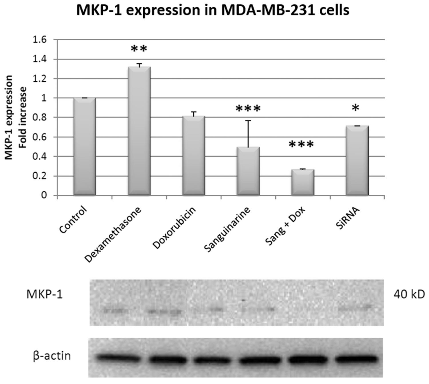
Volume 120| Number 3/4 March/April 2024 89 https://doi.org/10.17159/sajs.2024/14917 Research Article Doxorubicin with sanguinarine induces apoptosis in cancer cells Page 3 of 12
Figure 1: The expression of MKP-1 following treatment with the MKP-1 activator, Dex, the MKP-1 inhibitor, Sang, MKP-1 silencing with siRNA, and Dox. Data are expressed as mean ± SEM (n = 3). *p < 0.05 versus control, **p < 0.01 versus control, ***p < 0.001 versus control.
Research Article
Doxorubicin with sanguinarine induces apoptosis in cancer cells
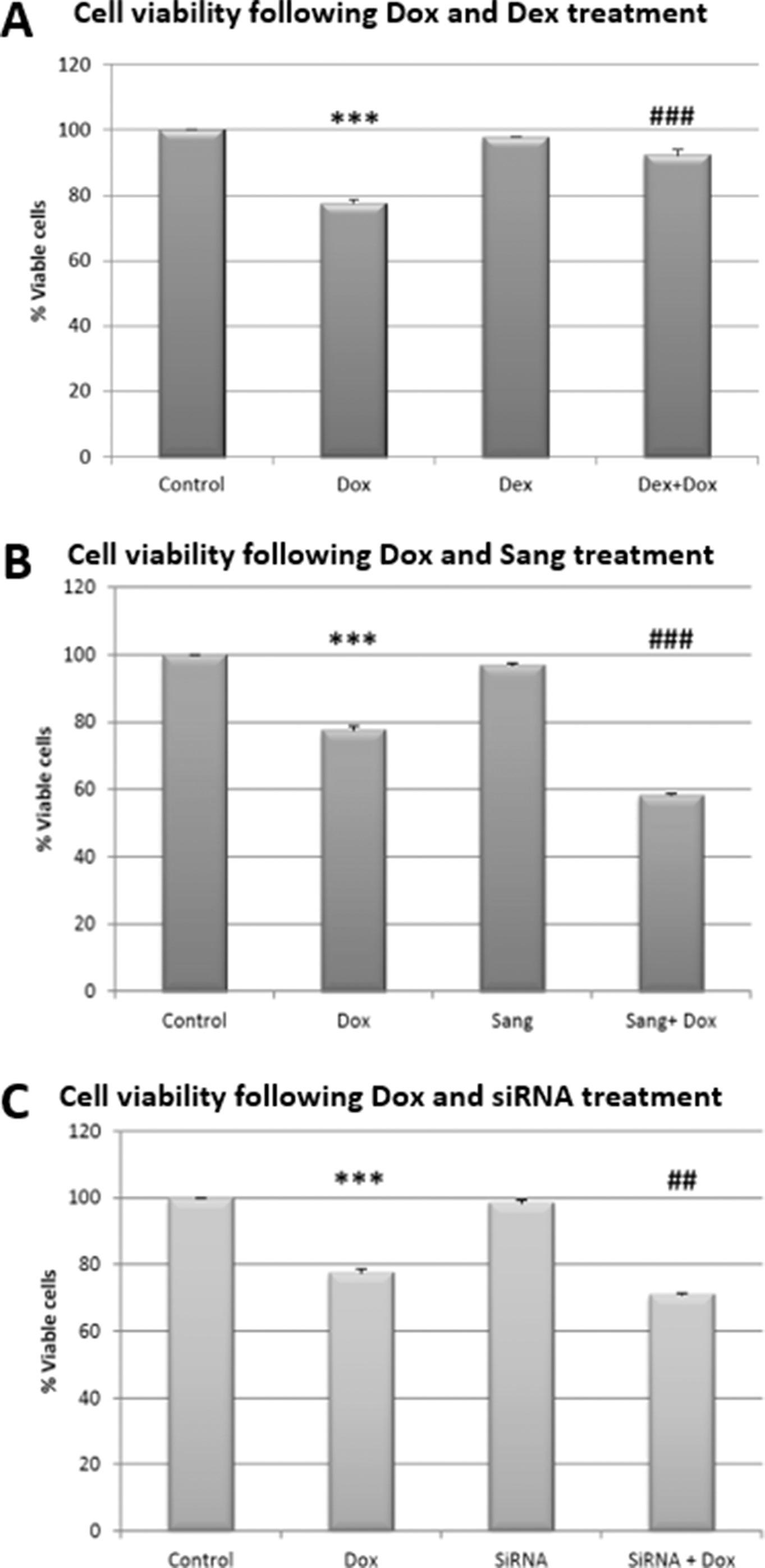
Volume 120| Number 3/4 March/April 2024 90 https://doi.org/10.17159/sajs.2024/14917
Page
12
4 of
Figure 2: The cell viability of MDA-MB-231 cells following treatment with the MKP-1 inducer, Dex, the MKP-1 inhibitor, Sang, MKP-1 silencing with siRNA, and Dox. (A) Cell viability following Dox and Dex treatment. (B) Cell viability following Dox and Sang treatment. (C) Cell viability following Dox and siRNA treatment. Data are expressed as mean ± SEM (n = 3). ***p < 0.001 versus control, ##p < 0.01 versus Dox, ###p < 0.001 versus Dox.
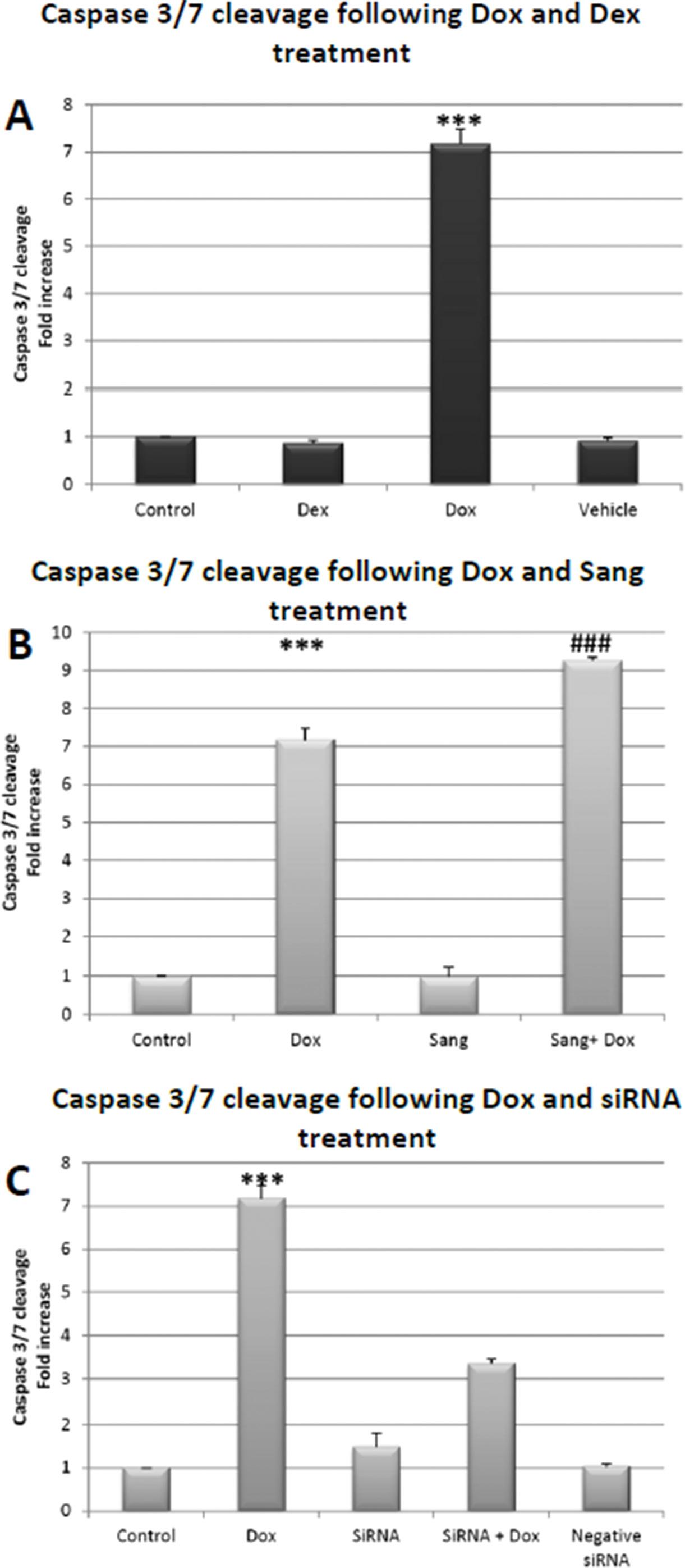
Volume 120| Number 3/4 March/April 2024 91 https://doi.org/10.17159/sajs.2024/14917
Article Doxorubicin with sanguinarine induces apoptosis in cancer cells Page 5 of 12
Research
Figure 3: Caspase-3/7 activity as a measure of apoptosis in MDA-MB-231 cells following treatment with the MKP-1 inducer, Dex, the MKP-1 inhibitor, Sang, MKP-1 silencing with siRNA, and Dox. (A) Caspase-3/7 activity following Dox and Dex treatment. (B) Caspase-3/7 activity following Dox and Sang treatment. (C) Caspase-3/7 activity following Dox and siRNA treatment. Data are expressed as mean ± SEM (n = 3). ***p < 0.001 versus control, ### p < 0.001 versus Dox.
assays. The activator of MKP-1, Dex, significantly increased caspase 3 expression when compared to the control (p < 0.01) without PARP cleavage. In contrast, the combination of Dox and Dex treatment resulted in the decreased expression of caspase 3 (p < 0.01) and increased cleavage of PARP (p < 0.001). Therefore, Dex confers protection against apoptosis, where the addition of Dox abolishes this effect. The inhibitor of MKP-1, Sang, resulted in no significant change in caspase 3
expression or PARP cleavage when compared to the control. However, the co-treatment of Sang and Dox resulted in a significant decrease in caspase 3 expression (p < 0.001) and PARP cleavage (p < 0.01) when compared to the Dox group, which is supported by our findings for the Caspase-Glo® 3/7 and viability assays. The expression of caspase 3 was significantly increased following treatment with MKP-1 siRNA when compared to the control (p < 0.05) with no change in PARP cleavage;
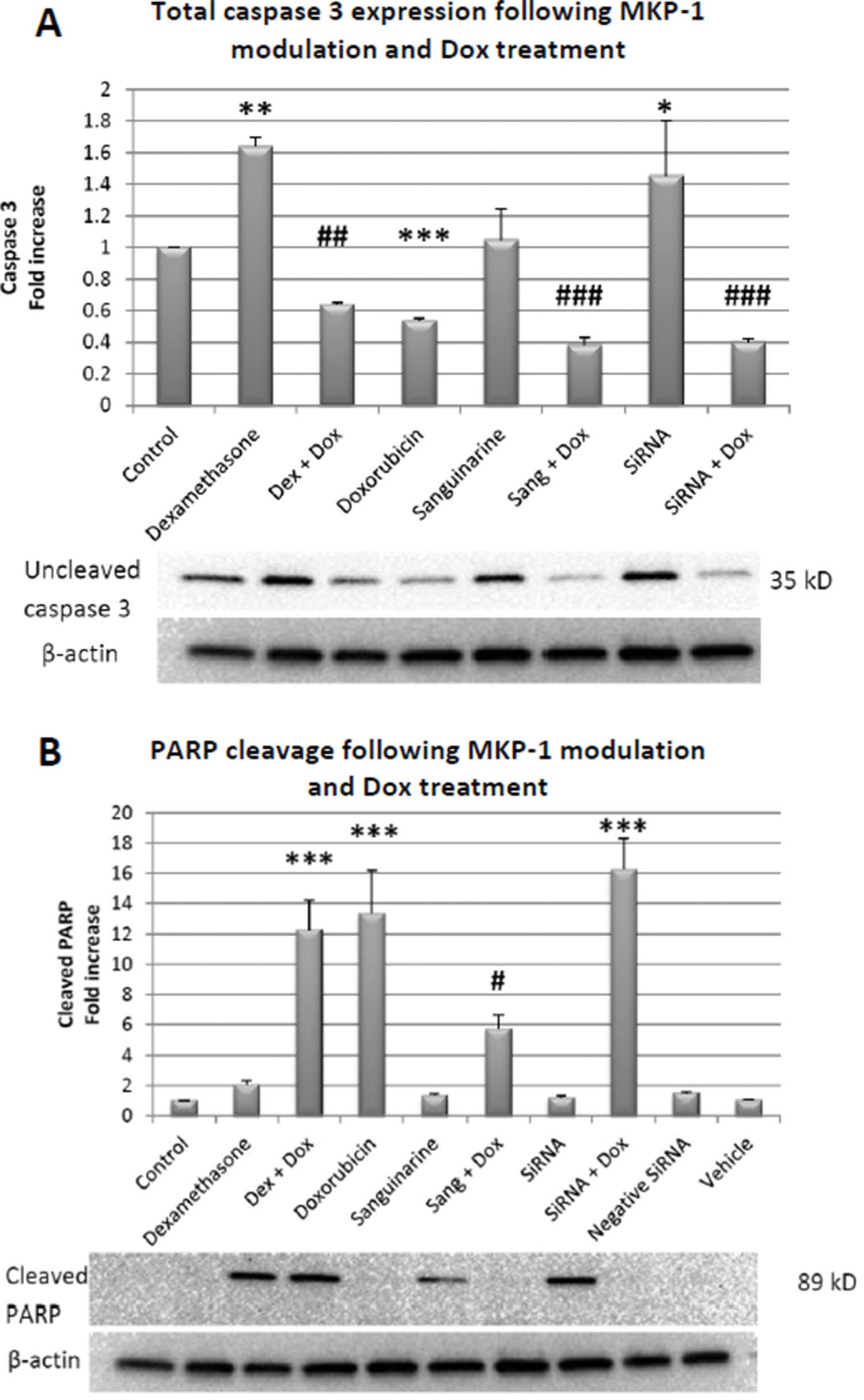
Volume 120| Number 3/4 March/April 2024 92 https://doi.org/10.17159/sajs.2024/14917
Research Article
Doxorubicin with sanguinarine induces apoptosis in cancer cells Page 6 of 12
Figure 4: The expression of caspase 3 and the cleavage of PARP as a measure of apoptosis in MDA-MB-231 cells following treatment with the MKP-1 inducer, Dex, the MKP-1 inhibitor, Sang, MKP-1 silencing with siRNA, and with Dox. (A) The expression of total caspase 3. (B) The cleavage of PARP. Data are expressed as mean ± SEM (n = 3). *p < 0.05 versus control, **p < 0.01 versus control, ***p < 0.001 versus control, #p < 0.05 versus Dox, ##p < 0.01 versus Dox, ###p < 0.001 versus Dox.
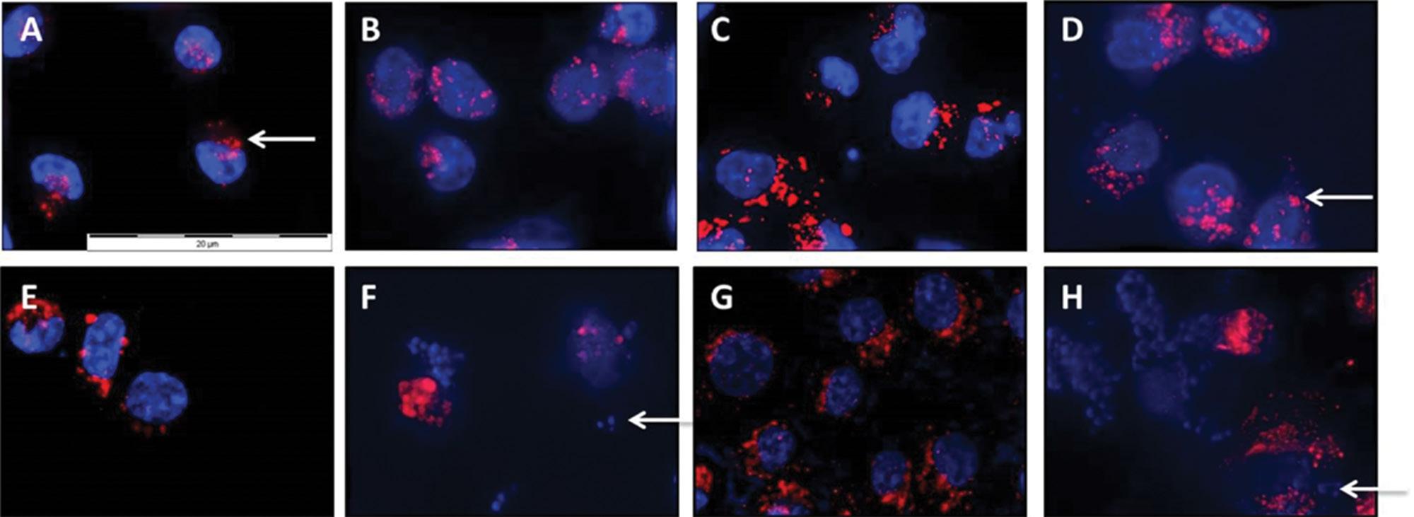
however, co-treatment with the MKP-1 silencer and Dox significantly reduced caspase 3 expression (p < 0.001), while increasing PARP cleavage (p < 0.001) when compared to Dox (Figure 4A,B). Therefore, MKP-1 inhibition and silencing sensitise breast cancer cells to apoptosis during Dox treatment.
MKP-1 inhibition and silencing during Dox treatment promotes changes in cell morphology
Morphological analysis revealed an increase in the size and number of acidic vesicles in response to both Sang and MKP-1 siRNA (Figure 5B), as well as in cells treated with both Sang and Dox (Figure 5F) or MKP-1 siRNA and Dox (Figure 5H). An increase in cell death markers, such as pyknosis and apoptotic bodies, was observed in the groups treated with Dex and Dox (Figure 5D) or MKP-1 siRNA and Dox (Figure 5H) where the highest degree of cell death was seen in the cells treated with Sang in combination with Dox (Figure 5F).
MKP-1 inhibition promotes autophagy
A significant increase in the conversion of LC3-1 to LC3-II was observed when MKP-1 was inhibited with Sang during Dox treatment when compared to Dox treatment alone (p < 0.01; Figure 6A). Furthermore, the expression of the cargo recruiter, p62/SQSTM1, was significantly increased in the Dex (p < 0.001) and Sang (p < 0.01) treated groups when compared to the control (Figure 6B). Evident in the increased conversion of LC3-1 to LC3-II and the twofold reduction in p62 expression, autophagy was induced.
Lysosomal acidic
compartments undergo differential changes under conditions of MKP-1 induction, inhibition and silencing during Dox treatment
Treatment with Dox significantly increased lysosomal acidic compartments compared to the control (p < 0.05; Figure 7A). Dex treatment, a known MKP-1 inducer, had no effect on lysosomal acidic compartments compared to the control. However, the combination treatment of Dex and Dox resulted in a significant increase in lysosomal acidic compartments compared to the control (p < 0.05), although to the same extent as Dox treatment alone (Figure 7A). Sang treatment alone and in combination with Dox did not result in a significant change in lysosomal acidic compartments (Figure 7B). MKP-1 siRNA resulted in no significant change in lysosomal acidic compartments when compared to the control (Figure 7C). However, a significant (p < 0.05) increase in lysosomal acidic compartments was observed with Dox in conjunction with MKP-1 siRNA compared to control.
Discussion
It is well established that MKP-1 is associated with cancer progression and resistance to chemotherapy.13,14 It has been reported that MKP-1 is overexpressed by more than fivefold in primary samples from breast cancer patients.32-34 We, therefore, investigated whether doxorubicin treatment and treatment with the MKP-1 inhibitor, sanguinarine, and silencing of MKP-1 using siRNA can inhibit MKP-1 expression in MDA-MB-231 cells (Figure 1). Doxorubicin treatment did not alter the expression levels of MKP-1, which is in contrast to a study performed by Rojo et al.35 who reported that doxorubicin decreased MKP-1 expression in a time- and dose-dependent manner. However, treatment with the glucocorticoid dexamethasone significantly increased MKP-1 expression in the MDA-MB-231 cells. This is supported by studies that confirmed that dexamethasone treatment is an inducer of MKP-1 expression.36,37 Additionally, we investigated whether the bioactive plant extract sanguinarine can inhibit MKP-1 expression in breast cancer cells. Treatment with sanguinarine significantly decreased the expression of MKP-1 in triple negative breast cancer cells. This is supported by a study performed by Vogt et al.26 in which sanguinarine treatment inhibited MKP-1 expression in PANC-1 and HeLa cells. Furthermore, the silencing of MKP-1 with MKP-1 siRNA also significantly decreased the expression of MKP-1 in vitro This confirmed dexamethasone as an inducer of MKP-1 expression, while sanguinarine and MKP-1 siRNA effectively inhibited MKP-1 expression. We also found that co-treatment with sanguinarine and doxorubicin inhibits the expression of MKP-1, which is supported by existing reports that both doxorubicin and sanguinarine are inhibitors of MKP-1 expression.10,26,35
Based on these findings, we investigated the effects of MKP-1 modulation on the viability and apoptosis of breast cancer cells following doxorubicin treatment in vitro. Doxorubicin treatment significantly decreased cell viability of breast cancer cells (Figure 2A–C), which is supported by our findings of the increased activity of caspase 3 and 7 in vitro (Figure 3A). Furthermore, doxorubicin treatment significantly decreased total caspase 3 and increased PARP cleavage (Figure 4A,B). It is therefore concluded that doxorubicin induced apoptosis in vitro in our model. The sensitivity of these cell lines to doxorubicin has also been well established where increased levels of apoptosis are evident following doxorubicin treatment.38-40 We then investigated whether the modulation of MKP-1 during doxorubicin treatment promotes or inhibits apoptosis induction in breast cancer cells. MKP-1 upregulation by dexamethasone alone did not affect cell viability or induce apoptosis (Figure 2A, 3A and 4), which is supported by previous studies which reported that glucocorticoids protect mammary gland epithelial cells, hepatocytes
Volume 120| Number 3/4 March/April 2024 93 https://doi.org/10.17159/sajs.2024/14917 Research Article Doxorubicin with sanguinarine induces apoptosis in cancer cells Page 7 of 12
Figure 5: The effect of 24-h Dox treatment in combination with MKP-1 inhibitors and inducers on autophagy and apoptosis in MDA-MB-231 cells. (A) Control, (B) Dox, (C) Dex, (D) Dex and Dox, (E) Sang, (F) Sang and Dox, (G) siRNA and (H) siRNA and Dox. Red fluorescence indicates LysoTracker™ red, while blue fluorescence indicates nuclei (Hoechst 33342). The arrows indicate apoptotic bodies (blue) and autophagic vacuoles (red).
Doxorubicin with sanguinarine induces apoptosis in cancer cells
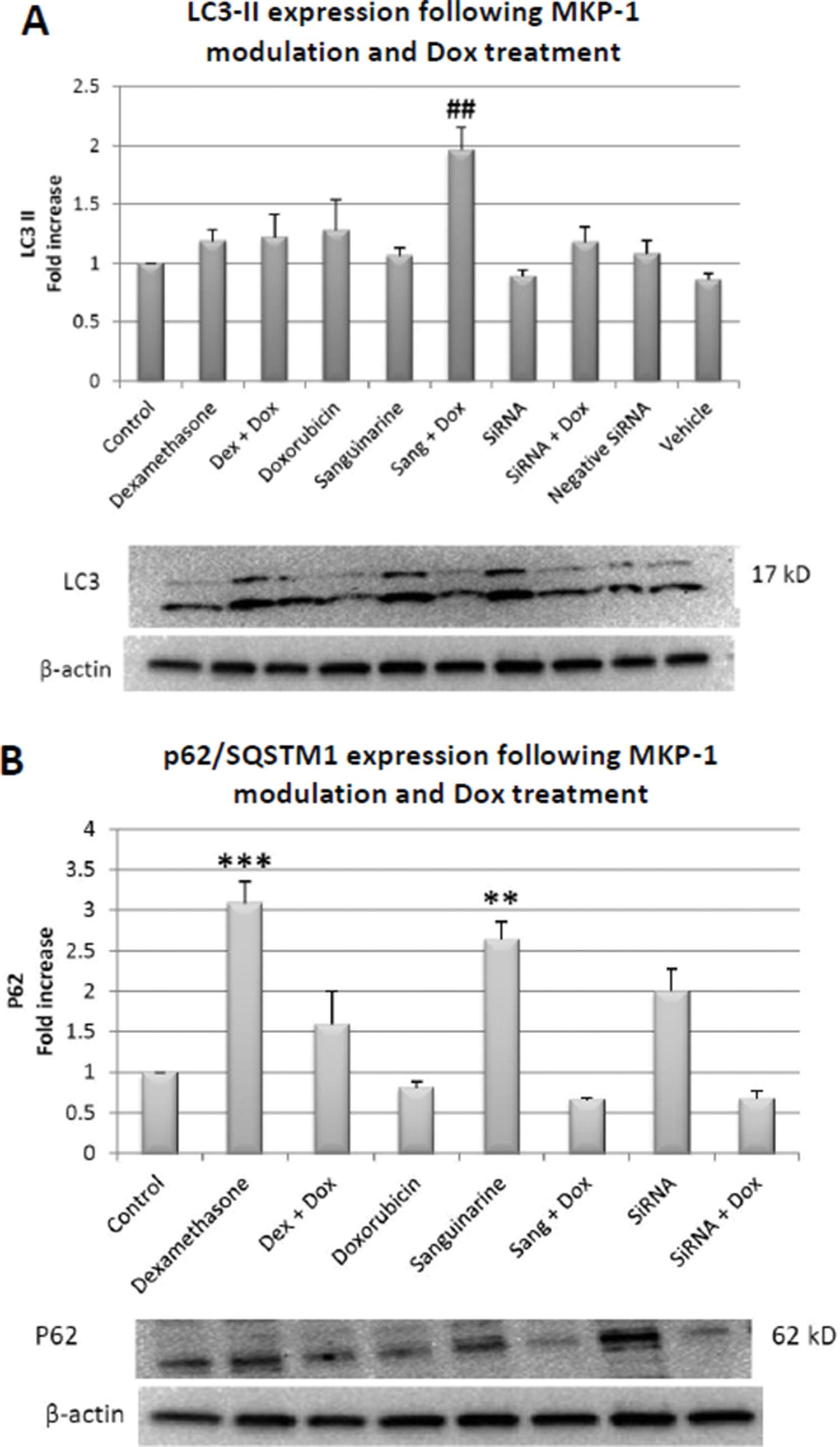
and ovarian follicular cells against cell death signals and apoptosis.41 This protective effect may be mediated by the upregulation of MKP-1, which can inhibit MAPK-induced apoptosis. However, co-treatment with
Research Article
https://doi.org/10.17159/sajs.2024/14917
dexamethasone and doxorubicin promoted cell death, indicating that the upregulation of MKP-1 alone confers a protective effect against apoptosis, but doxorubicin treatment abolishes this effect. Furthermore, the inhibition
Volume 120| Number 3/4 March/April 2024 94
Page 8 of 12
Figure 6: The expression of LC3-II and p62/SQSTM1 as a measure of autophagy in MDA-MB-231 cells following treatment with the MKP-1 inducer, Dex, the MKP-1 inhibitor, Sang, MKP-1 silencing with siRNA, and with Dox. (A) Treatment with Dox and Dex. (B) Treatment with Dox and Sang. (C) Treatment with Dox and siRNA. Data are expressed as mean ± SEM (n = 3). **p < 0.01 versus control, ***p < 0.001 versus control, ##p < 0.01 versus Dox.
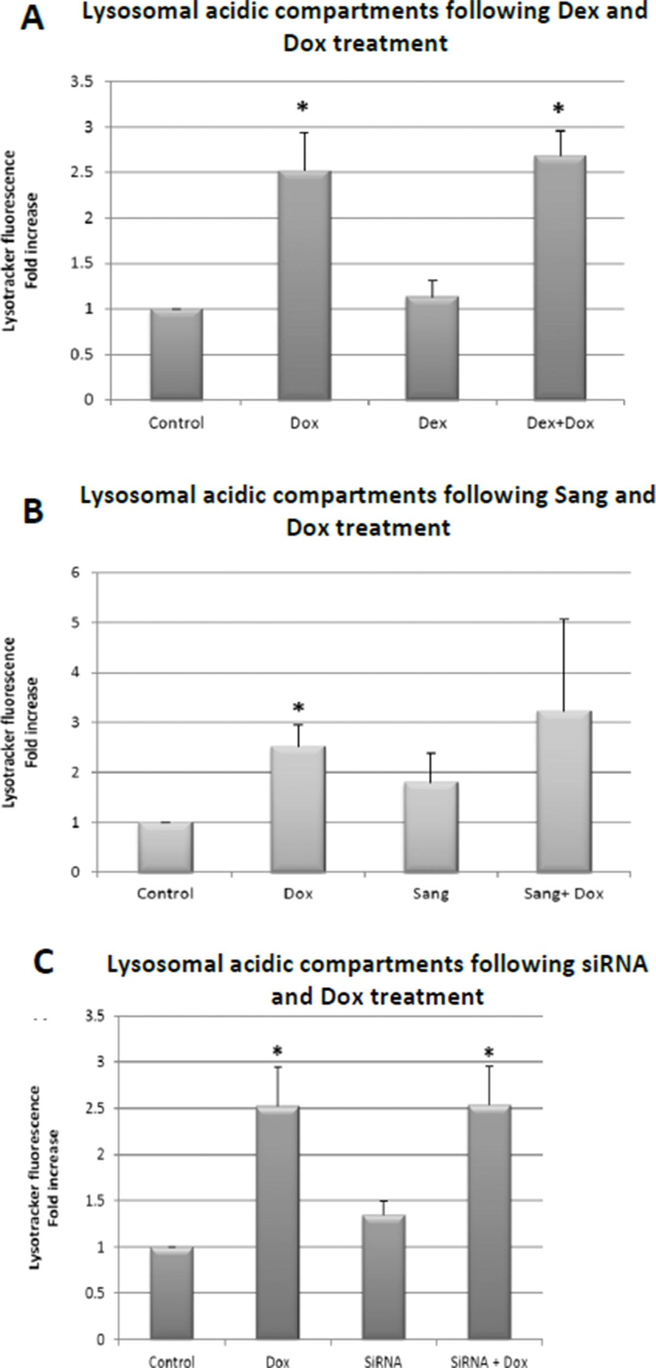
Volume 120| Number 3/4 March/April 2024 95 https://doi.org/10.17159/sajs.2024/14917
Article
Page 9 of 12
Research
Doxorubicin with sanguinarine induces apoptosis in cancer cells
Figure 7: Lysosomal acidic compartments in MDA-MB-231 cells following treatment with the MKP-1 inducer, Dex, the MKP-1 inhibitor, Sang, MKP-1 silencing with siRNA, and with Dox. (A) Treatment with Dox and Dex. (B) Treatment with Dox and Sang. (C) Treatment with Dox and siRNA. Data are expressed as mean ± SEM (n = 3). *p < 0.05.
of MKP-1 with sanguinarine alone did not affect breast cancer cell apoptosis (Figure 2B, 3B and 4A-B). This suggests that the inhibition of MKP-1 alone is not an effective inducer of apoptosis. However, it has been reported that sanguinarine inhibits cancer cell proliferation with different degrees of sensitivity in different triple negative breast cancer cell lines.42 43 Co-treatment with sanguinarine and doxorubicin decreased the amount of viable cancer cells and induced apoptosis (Figure 2B, 3B and 4A-B). These results indicate that sanguinarine improves the efficacy of doxorubicin treatment by sensitising breast cancer cells to doxorubicin-induced cell death in vitro This is supported by studies showing that MKP-1 inhibition induced apoptosis in cervical and renal cell carcinomas16, as well as in mesangial cells44. As with sanguinarine treatment, the silencing of MKP-1 with MKP-1 siRNA alone did not affect apoptosis (Figure 2C, 3C and 4B). However, the co-administration of doxorubicin and siRNA significantly decreased cell viability and induced apoptosis. This supports our findings for sanguinarine and doxorubicin co-treatment. Furthermore, Wang et al.45 reported that the inhibition of MKP-1 sensitised ovarian cancer cells to cisplatin-induced apoptosis, which is mediated through the activation of theMAPKs.Therefore,theinhibitionofMKP-1duringdoxorubicintreatment may have important therapeutic value. Various chemotherapeutic agents induce apoptosis through the activation of the MAPKs, namely ERK, JNK and p38. These MAPKs are negatively regulated by MKP-1. MAPKs are involved in apoptosis induction, and their activation by chemotherapies induces cytochrome c release from the mitochondria. This results in the oligomerisation of apoptotic protease activating factor-1 (Apaf-1), recruiting pro-caspase-9 and inducing its autoactivation, which results in the downstream activation of the effector caspase 3.46 Furthermore, JNK family members are involved in the activation of apoptosis by transcription-dependent processes, including death receptor induction.47 Therefore, loss or inhibition of MKP-1 reduces its inhibition on members of the MAPK family, which may facilitate apoptosis following doxorubicin treatment. Furthermore, Small and co-authors10 reported that MKP-1 inhibition enhanced chemosensitivity to doxorubicin through the activation of JNK. To further validate our findings for apoptosis, morphological changes commonly associated with the progression of apoptosis, such
as chromatin condensation and the formation of apoptotic bodies, were also investigated (Figure 5A–H). The doxorubicin-treated groups displayed increased morphological characteristics that are associated with cell death, including pyknosis and the formation of apoptotic bodies. Co-treatment with sanguinarine and doxorubicin displayed the highest degree of apoptosis induction when compared to the other treatment groups. This further supports our findings that under conditions of MKP-1 inhibition, MDA-MB-231 cells are sensitised to doxorubicin-induced apoptosis.
Autophagy has been shown to play a dual role in doxorubicin-induced cell death.48 We therefore assessed whether the modulation of MKP-1 and doxorubicin treatment can regulate autophagy. The co-administration of sanguinarine and doxorubicin induced autophagy in vitro (Figure 6A,B). This may be a synergistic effect between sanguinarine and doxorubicin, as treatment with sanguinarine or doxorubicin alone was not sufficient to induce autophagy. In line with this, sanguinarine has been reported to induce ROS-dependent autophagy and apoptosis in hepatocellular carcinoma cells.49 This may be mediated through the resulting upregulation of MAPK activity following MKP-1 inhibition. The MAPK family are known regulators of autophagy, either inducing or inhibiting autophagy. It has been reported that ERK activation can induce autophagy by promoting the dissociation of Beclin-1 and Bcl-2, through the direct activation of the Gα-interacting protein (GAIP) and through the activation of ATF4, resulting in the increased transcription of the ATG proteins.50-52 Furthermore, p38 activation can also induce autophagy through the activation of the ULK complex and LAMP2A translocation to the lysosomal membrane.53,54 Lastly, JNK activation promotes autophagy through the dissociation of Beclin-1 and Bcl-2, the direct activation of Atg5 and Atg7, and by inducing Sestrin2 transcription, which activates AMPK.55 Furthermore, at low doses, doxorubicin elicits an autophagic response in breast cancer cells.56 Additionally, increased levels of ATG2A mRNA have been observed following doxorubicin treatment57 , suggesting increased autophagy activation at the transcriptional level. Conversely, activation of autophagy in cultured cardiomyocytes following 1 μM doxorubicin treatment mediated its cardiotoxic effect.58 Here, it was shown that autophagy inhibition resulted in decreased cell death,
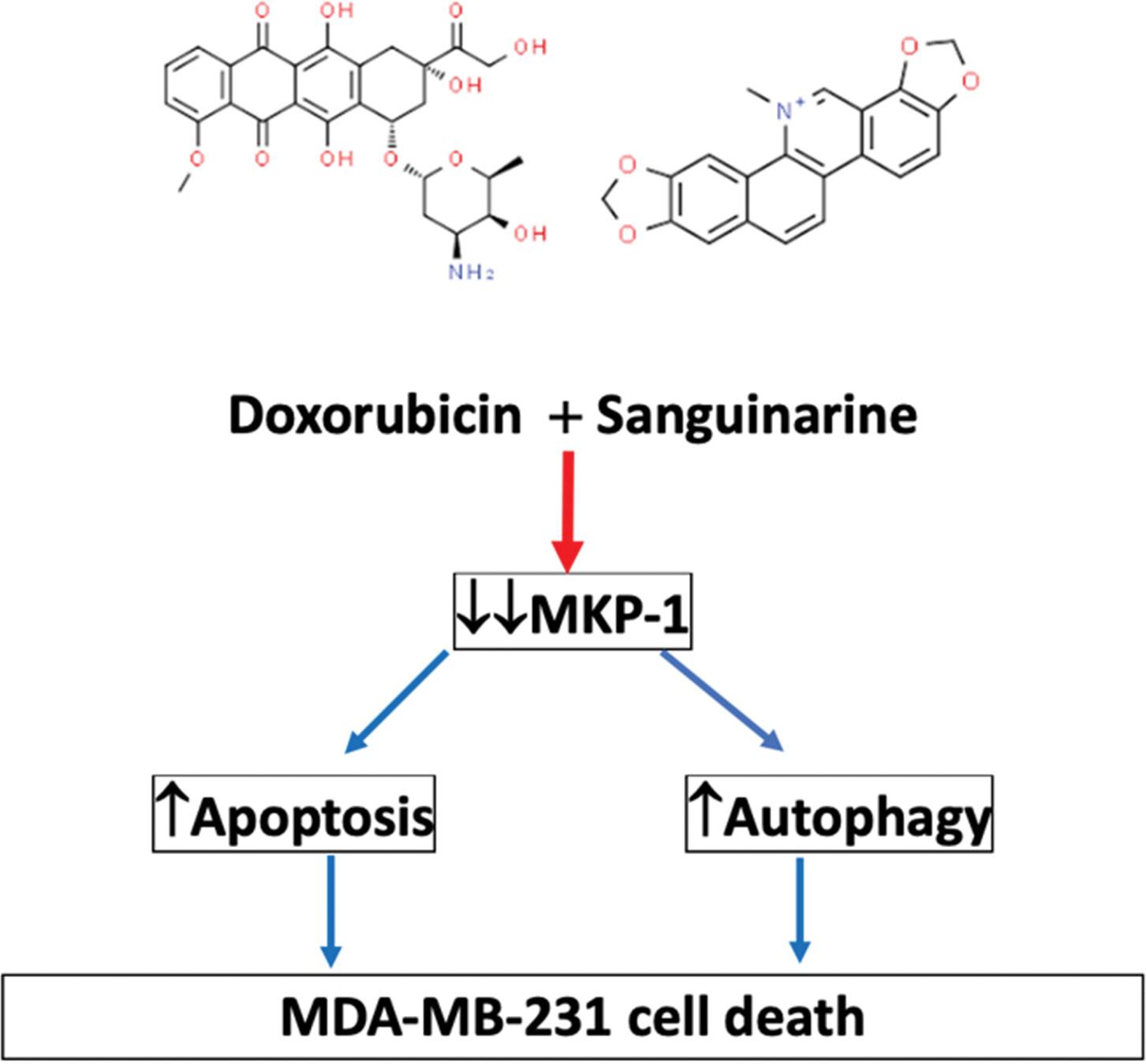
Volume 120| Number 3/4 March/April 2024 96 https://doi.org/10.17159/sajs.2024/14917 Research Article Doxorubicin with sanguinarine induces apoptosis in cancer cells Page 10 of 12
Figure 8: Proposed mechanism of action of doxorubicin and sanguinarine co-treatment in breast cancer cells.
and it was postulated that autophagy directly contributed to doxorubicininduced toxicity. Apoptosis and autophagy are finely regulated, and MKP-1 inhibition with sanguinarine may promote doxorubicin-induced apoptosis and autophagy as an anti-neoplastic mechanism. However, only doxorubicin, irrespective of MKP-1 modulation, induced an increase in lysosomal acidity (Figure 7A–C). This finding is in line with a study performed by Thomas et al.59 who showed that doxorubicin increased lysosomal acidity in MDA-MB-231 cells. Our results are also supported by the findings of other authors which show that doxorubicin induces an autophagic response in cancer cells.60 Figure 8 summarises the main findings of this study and the proposed mechanism of action of doxorubicin and sanguinarine in breast cancer cells.
Conclusions
We have reported a role for MKP-1 modulation during doxorubicin treatment in vitro. It is clear that both apoptosis and autophagy remain central in tumourigenesis. In conclusion, the findings of this study clearly indicate the significant role of MKP-1 in cancer treatment and the importance of modulating MKP-1 in a targeted way in cancer patients receiving chemotherapy.
Future perspectives
The role of MKP-1 in autophagy induction should be further explored to elucidate how the upregulation of autophagy can contribute to apoptosis. Future studies should assess autophagic flux over time and include autophagy inhibitors to quantify autophagosomal accumulation.
Acknowledgements
This work was supported by the National Research Foundation of South Africa (grant number 118566), the Cancer Association of South Africa and the South African Medical Research Council.
Competing interests
We have no competing interests to declare.
Authors’ contributions
M.d.P.: Writing – original draft, writing – review and editing. C.F.: Writing –review and editing. H.l.: Methodology, data collection, validation, sample and data analysis, data curation. A-M.E.: Conceptualisation, resources, writing – review and editing, supervision, funding acquisition, project leadership.
references
1. Mansoori B, Mohammadi A, Davudian S, Shirjang S, Baradaran B. The different mechanisms of cancer drug resistance: A brief review. Adv Pharm Bull. 2017;7(3):339–348. https://doi.org/10.15171/apb.2017.041
2. Crook T, Gaya A, Page R, Limaye S, Ranade A, Bhatt A, et al. Clinical utility of circulating tumor-associated cells to predict and monitor chemo-response in solid tumors. Cancer Chemother Pharmacol. 2021;87(2):197–205. https://d oi.org/10.1007/s00280-020-04189-8
3. Thorn CF, Oshiro C, Marsh S, Hernandez-Boussard T, McLeod H, Klein TE, et al. Doxorubicin pathways: Pharmacodynamics and adverse effects. Pharmacogenet Genomics. 2011;21(7):440–446. https://doi.org/10.1097/F PC.0b013e32833ffb56
4. Ferreira AL, Matsubara LS, Matsubara BB. Anthracycline-induced cardiotoxicity. Cardiovasc Hematol Agents Med Chem. 2008;6(4):278–281. https://doi.org/10 .2174/187152508785909474
5. Taymaz-Nikerel H, Karabekmez ME, Eraslan S, Kırdar B. Doxorubicin induces an extensive transcriptional and metabolic rewiring in yeast cells. Sci Rep. 2018;8(1):13672. https://doi.org/10.1038/s41598-018-31939-9
6. Octavia Y, Tocchetti CG, Gabrielson KL, Janssens S, Crijns HJ, Moens AL. Doxorubicin-induced cardiomyopathy: From molecular mechanisms to therapeutic strategies. J Mol Cell Cardiol. 2012;52(6):1213–1225. https://do i.org/10.1016/j.yjmcc.2012.03.006
7. Tacar O, Sriamornsak P, Dass CR. Doxorubicin: An update on anticancer molecular action, toxicity and novel drug delivery systems. J Pharm Pharmacol. 2013;65(2):157–170. https://doi.org/10.1111/j.2042-7158.2012.01567.x
Doxorubicin
8. Farooq A, Zhou MM. Structure and regulation of MAPK phosphatases. Cell Signal. 2004;16(7):769–779. https://doi.org/10.1016/j.cellsig.2003.12.008
9. Keyse SM. Dual-specificity MAP kinase phosphatases (MKPs) and cancer. Cancer Metastasis Rev. 2008;27(2):253–261. https://doi.org/10.1007/s105 55-008-9123-1
10. Small GW, Shi YY, Higgins LS, Orlowski RZ. Mitogen-activated protein kinase phosphatase-1 is a mediator of breast cancer chemoresistance. Cancer Res. 2007;67(9):4459–4466. https://doi.org/10.1158/0008-5472.CAN-06-2644
11. Vogt A, McDonald PR, Tamewitz A, Sikorski RP, Wipf P, Skoko JJ 3rd, et al. A cell-active inhibitor of mitogen-activated protein kinase phosphatases restores paclitaxel-induced apoptosis in dexamethasone-protected cancer cells. Mol Cancer Ther. 2008;7(2):330–340. https://doi.org/10.1158/1535-7 163.MCT-07-2165
12. Awada A, Albanell J, Canney PA, Dirix LY, Gil T, Cardoso F, et al. Bortezomib/ docetaxel combination therapy in patients with anthracycline-pretreated advanced/metastatic breast cancer: A phase I/II dose-escalation study. Br J Cancer. 2008;98(9):1500–1507. https://doi.org/10.1038/sj.bjc.6604347
13. MaG,Pan Y, Zhou C, Sun R, Bai J, Liu P, et al.Mitogen-activated protein kinase phosphatase 1 is involved in tamoxifen resistance in MCF7 cells. Oncol Rep. 2015;34(5):2423–2430. https://doi.org/10.3892/or.2015.4244
14. Lei S, Xu H, Chen N, Pan H, Xie W, He Y, et al. MKP-1 overexpression is associated with chemoresistance in bladder cancer via the MAPK pathway. Oncol Lett. 2020;20(2):1743–1751. https://doi.org/10.3892/ol.2020.11741
15. Shi YY, Small GW, Orlowski RZ. Proteasome inhibitors induce a p38 mitogenactivated protein kinase (MAPK)-dependent anti-apoptotic program involving MAPK phosphatase-1 and Akt in models of breast cancer. Breast Cancer Res Treat. 2006;100(1):33–47. https://doi.org/10.1007/s10549-006-9232-x
16. Mizuno R, Oya M, Shiomi T, Marumo K, Okada Y, Murai M. Inhibition of MKP-1 expression potentiates JNK related apoptosis in renal cancer cells. J Urol. 2004;172(2):723–727. https://doi.org/10.1097/01.ju.0000124990.37563.00
17. Franklin CC, Srikanth S, Kraft AS. Conditional expression of mitogen-activated protein kinase phosphatase-1, MKP-1, is cytoprotective against UV-induced apoptosis. Proc Natl Acad Sci USA. 1998;95(6):3014–3019. https://doi.org /10.1073/pnas.95.6.3014
18. Fu XH, Chen CZ, Li S, Han DX, Wang YJ, Yuan B, et al. Dual-specificity phosphatase 1 regulates cell cycle progression and apoptosis in cumulus cells by affecting mitochondrial function, oxidative stress, and autophagy. Am J Physiol Cell Physiol. 2019;317(6):C1183–C1193. https://doi.org/10. 1152/ajpcell.00012.2019
19. Degenhardt K, Mathew R, Beaudoin B, Bray K, Anderson D, Chen G, et al. Autophagy promotes tumor cell survival and restricts necrosis, inflammation, and tumorigenesis. Cancer Cell. 2006;10(1):51–64. https://doi.org/10.1016 /j.ccr.2006.06.001
20. Dasari SK, Bialik S, Levin-Zaidman S, Levin-Salomon V, Merrill AH Jr, Futerman AH, et al. Signalome-wide RNAi screen identifies GBA1 as a positive mediator of autophagic cell death. Cell Death Differ. 2017;24(7):1288–1302. https://doi.org/10.1038/cdd.2017.80
21. LiuPF,TsaiKL,HsuCJ,TsaiWL,ChengJS,ChangHW,etal.Drugrepurposing screening identifies tioconazole as an Atg4 inhibitor that suppresses autophagy and sensitizes cancer cells to chemotherapy. Theranostics. 2018;8(3):830–845. https://doi.org/10.7150/thno.22012
22. Aburai N, Yoshida M, Ohnishi M, Kimura K. Sanguinarine as a potent and specific inhibitor of protein phosphatase 2C in vitro and induces apoptosis via phosphorylation of p38 in HL60 cells. Biosci Biotechnol Biochem. 2010;74(3):548–552. https://doi.org/10.1271/bbb.90735
23. Jang BC, Park JG, Song DK, Baek WK, Yoo SK, Jung KH, et al. Sanguinarine induces apoptosis in A549 human lung cancer cells primarily via cellular glutathione depletion. Toxicol In Vitro. 2009;23(2):281–287. https://doi.org /10.1016/j.tiv.2008.12.013
24. Park H, Bergeron E, Senta H, Guillemette K, Beauvais S, Blouin R, et al. Sanguinarine induces apoptosis of human osteosarcoma cells through the extrinsic and intrinsic pathways. Biochem Biophys Res Commun. 2010;399(3):446–451. https://doi.org/10.1016/j.bbrc.2010.07.114
25. Serafim TL, Matos JA, Sardão VA, Pereira GC, Branco AF, Pereira SL, et al. Sanguinarine cytotoxicity on mouse melanoma K1735-M2 cells-nuclear vs. mitochondrial effects. Biochem Pharmacol. 2008;76(11):1459–1475. https: //doi.org/10.1016/j.bcp.2008.07.013
Volume 120| Number 3/4 March/April 2024 97 https://doi.org/10.17159/sajs.2024/14917
Research Article
with sanguinarine induces apoptosis in cancer cells Page
12
11 of
26. Vogt A, Tamewitz A, Skoko J, Sikorski RP, Giuliano KA, Lazo JS. The benzo[c]phenanthridine alkaloid, sanguinarine, is a selective, cell-active inhibitor of mitogen-activated protein kinase phosphatase-1. J Biol Chem. 2005;280(19):19078–19086. https://doi.org/10.1074/jbc.M501467200
27. Adhami VM, Aziz MH, Reagan-Shaw SR, Nihal M, Mukhtar H, Ahmad N. Sanguinarine causes cell cycle blockade and apoptosis of human prostate carcinoma cells via modulation of cyclin kinase inhibitor-cyclin-cyclindependent kinase machinery. Mol Cancer Ther. 2004;3(8):933–940. https: //doi.org/10.1158/1535-7163.933.3.8
28. Xu J, Meng Q, Chong Y, Jiao Y, Zhao L, Rosen EM. Sanguinarine inhibits growth of human cervical cancer cells through the induction of apoptosis. Oncol Rep. 2012;28:2264–2270. https://doi.org/10.3892/or.2012.2024
29. AhsanH,Reagan-ShawS,BreurJ,AhmadN.Sanguinarineinducesapoptosis of human pancreatic carcinoma AsPC-1 and BxPC-3 cells via modulations in Bcl-2 family proteins. Cancer Lett. 2007;249(2):198–208. https://doi.org/10 .1016/j.canlet.2006.08.018
30. Kitakaze M, Fong M, Yoshitake M, Minamino T, Node K, Okuyama Y, et al. Vesnarinone inhibits adenosine uptake in endothelial cells, smooth muscle cells and myocytes, and mediates cytoprotection. J Mol Cell Cardiol. 1997;29(12):3413–3417. https://doi.org/10.1006/jmcc.1997.0581
31. Bradford MM. A rapid and sensitive method for the quantitation of microgram quantities of protein utilizing the principle of protein-dye binding. Anal Biochem. 1976;72:248–254. https://doi.org/10.1006/abio.1976.9999
32. Wang HY, Cheng Z, Malbon CC. Overexpression of mitogen-activated protein kinase phosphatases MKP1, MKP2 in human breast cancer. Cancer Lett. 2003;191(2):229–237. https://doi.org/10.1016/S0304-3835(02)00612-2
33. Loda M, Capodieci P, Mishra R, Yao H, Corless C, Grigioni W, et al. Expression of mitogen-activated protein kinase phosphatase-1 in the early phases of human epithelial carcinogenesis. Am J Pathol. 1996;149(5):1553–1564.
34. Kurt RA, Urba WJ, Smith JW, Schoof DD. Peripheral T lymphocytes from women with breast cancer exhibit abnormal protein expression of several signalling molecules. Int J Cancer. 1998;78(1):16–20. https://doi.org/10.100 2/(SICI)1097-0215(19980925)78:1<16::AID-IJC4>3.0.CO;2-#
35. Rojo F, González-Navarrete I, Bragado R, Dalmases A, Menéndez S, CortesSempere M, et al. Mitogen-activated protein kinase phosphatase-1 in human breast cancer independently predicts prognosis and is repressed by doxorubicin. Clin Cancer Res. 2009;15(10):3530–3539. https://doi.org/10.1 158/1078-0432.CCR-08-2070
36. Chen P, Li J, Barnes J, Kokkonen GC, Lee JC, Liu Y. Restraint of proinflammatory cytokine biosynthesis by mitogen-activated protein kinase phosphatase-1 in lipopolysaccharide-stimulated macrophages. J Immunol. 2002;169(11):6408–6416. https://doi.org/10.4049/jimmunol.169.11.6408
37. Clark AR. MAP kinase phosphatase 1: A novel mediator of biological effects of glucocorticoids? J Endocrinol. 2003;178(1):5–12. https://doi.org/10.167 7/joe.0.1780005
38. Aroui S, Brahim S, De Waard M, Bréard J, Kenani A. Efficient induction of apoptosis by doxorubicin coupled to cell-penetrating peptides compared to unconjugated doxorubicin in the human breast cancer cell line MDA-MB 231. Cancer Lett. 2009;285(1):28–38. https://doi.org/10.1016/j.canlet.2009.04.044
39. Kim TH, Shin YJ, Won AJ, Lee BM, Choi WS, Jung JH, et al. Resveratrol enhanceschemosensitivityofdoxorubicininmultidrug-resistanthumanbreast cancer cells via increased cellular influx of doxorubicin. Biochim Biophys Acta. 2014;1840(1):615–625. https://doi.org/10.1016/j.bbagen.2013.10.023
40. Mussi SV, Sawant R, Perche F, Oliveira MC, Azevedo RB, Ferreira LA, et al. Novel nanostructured lipid carrier co-loaded with doxorubicin and docosahexaenoicaciddemonstratesenhancedinvitroactivityandovercomes drug resistance in MCF-7/Adr cells. Pharm Res. 2014;31(8):1882–1892. https://doi.org/10.1007/s11095-013-1290-2
41. Redondo M, Téllez T, Roldan MJ, Serrano A, García-Aranda M, Gleave ME, et al. Anticlusterin treatment of breast cancer cells increases the sensitivities of chemotherapy and tamoxifen and counteracts the inhibitory action of dexamethasone on chemotherapy-induced cytotoxicity. Breast Cancer Res. 2007;9(6):R86. https://doi.org/10.1186/bcr1835
42. Ghauri MA, Su Q, Ullah A, Wang J, Sarwar A, Wu Q, et al. Sanguinarine impedes metastasis and causes inversion of epithelial to mesenchymal transition in breast cancer. Phytomedicine. 2021;84, Art. #153500. https://d oi.org/10.1016/j.phymed.2021.153500
Doxorubicin with sanguinarine induces apoptosis in cancer cells Page 12 of
43. Messeha S, Zarmouh N, Noel S, Soliman K. Gene expression alterations associated with sanguinarine -induced antiproliferative effect and apoptosis in triple-negative breast cancer cells. FASEB J. 2021;35(S1). https://doi.org/ 10.1096/fasebj.2021.35.S1.00463
44. Xu Q, Konta T, Nakayama K, Furusu A, Moreno-Manzano V, Lucio-Cazana J, et al. Cellular defense against H2O2-induced apoptosis via MAP kinase-MKP-1 pathway. Free Radic Biol Med. 2004;36(8):985–993. https://doi.org/10.1016 /j.freeradbiomed.2004.01.009
45. Wang Z, Xu J, Zhou JY, Liu Y, Wu GS. Mitogen-activated protein kinase phosphatase-1 is required for cisplatin resistance. Cancer Res. 2006;66(17): 8870–8877. https://doi.org/10.1158/0008-5472.CAN-06-1280
46. Aoki H, Kang PM, Hampe J, Yoshimura K, Noma T, Matsuzaki M, et al. Direct activation of mitochondrial apoptosis machinery by c-Jun N-terminal kinase in adult cardiac myocytes. J Biol Chem. 2002;277(12):10244–10250. https: //doi.org/10.1074/jbc.M112355200
47. Roos WP, Kaina B. DNA damage-induced cell death by apoptosis. Trends Mol Med. 2006;12(9):440–450. https://doi.org/10.1016/j.molmed.2006.07.007
48. Koleini N, Kardami E. Autophagy and mitophagy in the context of doxorubicininduced cardiotoxicity. Oncotarget. 2017;8(28):46663–46680. https://doi.or g/10.18632/oncotarget.16944
49. Wang J, Su Q, Wu Q, Chen K, Ullah A, Ghauri MA, et al. Sanguinarine impairs lysosomal function and induces ROS-dependent mitophagy and apoptosis in human hepatocellular carcinoma cells. Arch Pharm Res. 2021;44(11):1025–1036. https://doi.org/10.1007/s12272-021-01356-0
50. Feng W, Huang S, Wu H, Zhang M. Molecular basis of Bcl-xL’s target recognition versatility revealed by the structure of Bcl-xL in complex with the BH3 domain of Beclin-1. J Mol Biol. 2007;372(1):223–235. https://doi.org/1 0.1016/j.jmb.2007.06.069
51. Shin S, Buel GR, Wolgamott L, Plas DR, Asara JM, Blenis J, et al. ERK2 mediates metabolic stress response to regulate cell fate. Mol Cell. 2015;59(3):382–398. https://doi.org/10.1016/j.molcel.2015.06.020
52. Zheng W, Xie W, Yin D, Luo R, Liu M, Guo F. ATG5 and ATG7 induced autophagy interplays with UPR via PERK signaling. Cell Commun Signal. 2019;17(1):42. https://doi.org/10.1186/s12964-019-0353-3
53. Slobodnyuk K, Radic N, Ivanova S, Llado A, Trempolec N, Zorzano A, et al. Autophagy-induced senescence is regulated by p38α ignalling. Cell Death Dis. 2019;10(6):376. https://doi.org/10.1038/s41419-019-1607-0
54. Li W, Zhu J, Dou J, She H, Tao K, Xu H, et al. Phosphorylation of LAMP2A by p38 MAPK couples ER stress to chaperone-mediated autophagy. Nat Commun. 2017;8(1):1763. https://doi.org/10.1038/s41467-017-01609-x
55. Zhang XY, Wu XQ, Deng R, Sun T, Feng GK, Zhu XF. Upregulation of sestrin 2 expression via JNK pathway activation contributes to autophagy induction in cancer cells. Cell Signal. 2013;25(1):150–158. https://doi.org/10.1016/j.ce llsig.2012.09.004
56. Akar U, Chaves-Reyez A, Barria M, Tari A, Sanguino A, Kondo Y, et al. Silencing of Bcl-2 expression by small interfering RNA induces autophagic cell death in MCF-7 breast cancer cells. Autophagy. 2008;4(5):669–679. https://doi.org/10.4161/auto.6083
57. Levy JM, Thorburn A. Targeting autophagy during cancer therapy to improve clinical outcomes. Pharmacol Ther. 2011;131(1):130–141. https://doi.org/1 0.1016/j.pharmthera.2011.03.009
58. Kobayashi S, Volden P, Timm D, Mao K, Xu X, Liang Q. Transcription factor GATA4 inhibits doxorubicin-induced autophagy and cardiomyocyte death. J Biol Chem. 2010;285(1):793–804. https://doi.org/10.1074/jbc.M109.070037
59. Thomas M, Davis T, Nell T, Sishi B, Engelbrecht AM. Amino acid starvation sensitizes resistant breast cancer to doxorubicin-induced cell death. Front Cell Dev Biol. 2020;8, Art. #565915. https://doi.org/10.3389/fcell.2020.5 65915
60. LambertLA,QiaoN,HuntKK,LambertDH,MillsGB,MeijerL,etal.Autophagy: A novel mechanism of synergistic cytotoxicity between doxorubicin and roscovitine in a sarcoma model. Cancer Res. 2008;68(19):7966–7974. http s://doi.org/10.1158/0008-5472.CAN-08-1333
Volume 120| Number 3/4 March/April 2024 98
https://doi.org/10.17159/sajs.2024/14917 Research Article
12
AuthorS:
Simoné Karels1
Cecil Felix1
Sivakumar Pasupathi1
AFFILIAtIoN:
1South African Institute for Advanced Materials Chemistry (SAIAMC), University of the Western Cape, Cape Town, South Africa
CorrESPoNDENCE to:
Simoné Karels
EMAIL:
simonekarels2012@gmail.com
DAtES:
received: 19 May 2023
revised: 04 Dec. 2023
Accepted: 09 Dec. 2023
Published: 27 Mar. 2024
hoW to CItE:
Karels S, Felix C, Pasupathi S. Development of unsupported IrO2 nano-catalysts for polymer electrolyte membrane water electrolyser applications. S Afr J Sci. 2024;120(3/4), Art. #16026. https:// doi.org/10.17159/sajs.2024/16026
ArtICLE INCLuDES:
☒ Peer review
☐ Supplementary material
DAtA AVAILABILItY:
☐ Open data set
☒ All data included
☐ On request from author(s)
☐ Not available
☐ Not applicable
EDItor:
Priscilla Baker
KEYWorDS:
iridium oxide, oxygen evolution reaction, modified Adams fusion method, polymer electrolyte membrane water electrolyser, molten salt method
FuNDING:
South African Department of Trade, Industry and Competition (THRIP/19/31/08/2018)
Development of unsupported IrO2 nano-catalysts for polymer electrolyte membrane water electrolyser applications
IrO2 is a current state-of-the-art catalyst for polymer electrolyte membrane water electrolyser (PEMWE) applications due to its high stability during the oxygen evolution reaction (OER). However, its activity needs to be significantly improved to justify the use of such a high-cost material. In this study, the activity of the IrO2 catalyst was improved by optimising and comparing two synthesis methods: the modified Adams fusion method (MAFM) and the molten salt method (MSM). Optimum OER performances of the IrO2 catalysts synthesised with the two synthesis methods were obtained at different temperatures. For the MAFM, a synthesis temperature of 350 °C produced the IrO2 catalyst with an overpotential of 279 mV and the highest OER stability of 82 h at 10 mAcm−2. However, for the MSM, the lowest overpotential of 271 mV was observed for IrO2 synthesised at 350 °C, while the highest stability of 75 h was obtained for the IrO2 synthesised at 500 °C.
Significance:
IrO2 is still currently a state-of-the-art catalyst in PEMWE due to its high stability in the highly acidic and oxidising conditions of the OER. High-performance IrO2 catalysts were successfully produced via the MAFM and MSM. Both the MAFM and MSM are simple and easily scalable for high-volume production of metal oxide catalysts. This study showed that the physical/structural properties of the IrO2 catalysts can be tailored through synthesis methods and synthesis conditions to improve their OER performance.
Introduction
The polymer electrolyte membrane water electrolyser (PEMWE) is an important technology to produce hydrogen (H2) from renewable energy sources, i.e. green H2, due to its adaptability to the intermittent energy profiles of renewable energy sources like solar and wind power. However, the high costs associated with PEMWE components have remained a major challenge for the commercialisation of the technology. The high cost of the catalyst is of particular importance as it accounts for about 25% of the total catalyst-coated membrane cost. Furthermore, the catalyst-coated membrane shares about 24% of the total PEMWE stack cost.1 The oxygen evolution reaction (OER) is a four-electron process dominated by sluggish electrode kinetics, leading to high overpotentials.2 Therefore, the anodic catalyst in the PEMWE needs to be especially active and stable under the acidic OER environment to reduce the high overpotential. Expensive precious metals and their respective oxides are still known to be the most active and stable towards the OER although alternative non-precious metal materials are being investigated.3 While high activities are obtained from nonprecious metal catalysts, major challenges such as long-term stability need to be addressed before employing these materials as electrodes for large-scale, practical applications.4 Metal oxides based on Ir and Ru are considered stateof-the-art catalysts for the OER because of their high activity and stability.2 The IrO2 catalyst has low overpotential, maintains high stability in acidic media, is corrosion resistant, and has a high selectivity towards oxygen evolution.5 Wáng et al.6 summarised the ex-situ OER performances of various materials that incorporated either Ir or Ru into its matrix. A second-best performance was obtained with Ir0.06Co2.94O4 on an Au electrode exhibiting an overpotential of 250 mV and a stability of 200 h at 10 mVcm−2. However, it should be noted that the best performance obtained on a glassy carbon electrode (GCE) (out of 24 studies) was for a/c-RuO2, which exhibited a 205 mV overpotential and a stability of 60 h at 10 mVcm−2 . 7 The best performance for a monometallic Ir catalyst on a GCE was for mesoporous Ir nanosheets exhibiting an overpotential of 240 mV and a stability of 8 h at 10 mA/cm2. These findings might suggest that the working electrode type has a significant impact on the measured OER performances.
In this study, the IrO2 catalysts were developed via two methods: a modified Adams fusion method (MAFM) and a molten salt method (MSM). Although IrO2 is a commonly used catalyst in the PEMWE, its OER activity needs to be significantly improved to justify the use of such an expensive material. The OER performance of the catalyst depends critically on its morphology, shape and crystal structure.2,8 Besides optimising the physical properties of IrO2, the synthesis methods need to be cost-effective, easily scalable, green and clean.8 Since the introduction of the Adams fusion method in 1923 by Roger Adams and Ralph Shriner9, the method has been modified and adapted to synthesise various metal oxides including single, binary and ternary metal oxides, supported and unsupported metal oxides as well as adding chemical modifiers to improve the physical properties of the catalysts.4,10-14 Researchers have used various metals, reagent salts and synthesis temperatures to synthesise various metal oxides.15 During the MAFM, the temperature used causes the NaNO3 to melt and react with the Ir precursor. The synthesis temperature is always set to at least above the melting point of NaNO3, i.e., above 308 °C. The MSM is also a simple, cost-effective, easily scalable and eco-friendly method for the synthesis of metal oxide catalysts.8 During the MSM, the metal chloride precursor decomposes on the NaCl/KCl salt bed. The NaCl/KCl salt bed does not chemically react with the Ir precursor but acts as a support for the thermal decomposition of the Ir precursor in air. The synthesis temperature is mostly kept at 650 °C, which is below the melting point of the NaCl/KCl salt mixture.12 Previous studies suggested the MAFM IrO2 catalysts showed improved OER performance compared to MSM IrO2 catalysts.10,16 In this study, the MAFM and MSM were optimised by varying the synthesis temperatures, and the results were directly compared. Moreover, the reaction time of the MSM was reduced to 4 h (typically 12 h) and only NaCl was used as the salt bed.16 The MAFM and MSM were compared by examining the
Research Article
99 https://doi.org/10.17159/sajs.2024/16026 Volume 120| Number 3/4 March/April 2024 © 2024. The Author(s). Published under a Creative Commons Attribution Licence.
physical and electrochemical properties of the synthesised IrO2 catalysts. The IrO2 catalysts were physically characterised using X-ray diffraction (XRD), high-resolution transmission electron microscopy (HRTEM) and Brunauer–Emmett–Teller (BET) analyses. The IrO2 catalysts' OER performances were evaluated ex-situ via cyclic voltammetry (CV), linear sweep voltammetry (LSV) and chronopotentiometry (CP).
Methods
Electrocatalyst synthesis
Modified Adams fusion method
An amount of 0.36 g H2IrCl6 (SA Precious Metals) was dissolved in 10 mL isopropanol (Sigma) and magnetically stirred for 30 min. Thereafter, 3.6 g of finely ground NaNO3 (Alfa Aesar) sample was added to the solution and stirred for an additional 30 min. Excess solvent was evaporated on a hot plate followed by further drying in an oven set to 90 °C, for 30 min. The dried H2IrCl6/NaNO3 mixture was then reacted in a pre-heated furnace for 2 h to produce the IrO2 sample. The furnace temperatures selected for IrO2 synthesis were 350 °C, 500 °C and 650 °C. The obtained IrO2 sample was cooled, rinsed and filtered three times with 500 mL of ultrapure water (Milli Q) to remove the unreacted NaNO3 salt. A 0.1 M AgNO3 solution was used to ensure no chloride was present in the filtrate of the final 500 mL ultrapure water rinse/filter. After filtration, the IrO2 sample was dried in an oven for 4 h at 85 °C and then cooled down overnight inside the oven. A commercial IrO2 (Alfa Aesar) was used for comparison purposes. The samples synthesised using the MAFM are represented as MAFM-350, MAFM-500 and MAFM-650 to denote the different synthesis temperatures. Equations 1 and 2 show the suggested reactions occurring during the MAFM to produce the IrO2 catalyst.17
H2 IrCl6 + 6NaNO3 → 6NaCl + Ir (NO3)4 + 2HNO3 Equation 1
Ir (NO3)4 → IrO2 + 4NO3 + O2 Equation 2
Molten salt method
An amount of 0.4 g of H2IrCl6 (SA Precious Metals) and 15 g of NaCl (Laborem Lab Supplies) was grounded together for 15 min with a pestle and mortar. The H2IrCl6/NaCl mixture was then transferred to a crucible and reacted in a pre-heated furnace for 4 h. Furnace temperatures selected for IrO2 synthesis were 350 °C, 500 °C and 650 °C. Filtration, rinsing and drying were the same as for the MAFM. The samples synthesised using the MSM are represented as MSM-350, MSM-500 and MSM-650 to denote the different synthesis temperatures. A commercial IrO2 (Alfa Aesar) was used for comparison purposes.
Preparation of the working electrode
A Metrohm rotating disc electrode (RDE) setup fitted with a GCE (0.1963 cm2 working area) was used for the electrochemical analyses. The GCE was cleaned with 0.05 µm alumina paste (Buehler), polished and dried
before use. The catalyst inks were prepared by ultrasonically dispersing 8 mg of the IrO2 catalyst, 50 µL 5 wt% Nafion® solution (Alfa Aesar) and 1950 µL ultrapure water for 20 min. A micropipette was used to drop 30 µL of the IrO2 catalyst ink onto the GCE. The working electrode was covered with a glass beaker and dried for 24 h at ambient conditions. A calculated catalyst loading of 0.45 mg cm2 was obtained.
Physical characterisation
XRDwasperformedwiththeBrukerAXSD8AdvancediffractometerusingCu K radiation (λ = 1.5406 Å) operating at 40 kV and 40 mA. The IrO2 standard (JCP2_150870) was used for peak allocation. HRTEM was obtained using an FEI/Tecnai T20 operating at 200 kV. BET surface area analyses were performed using the Micromeritics 3 Flex surface characterisation analyser.
Electrochemical characterisation
Ex-situ electrochemical analyses were performed in a three-electrode setup at 25 °C and 1 atm. The Autolab potentiostat PGSTAT302N (Metrohm) was used for all electrochemical analyses. A circulating water bathwasusedtomaintainthetemperatureoftheelectrochemicalcell.The working electrode (described in 2.2), a 3 M Ag/AgCl reference electrode (Metrohm), a Pt metal sheet (1 cm2 area) counter electrode (Metrohm), which is five times larger than the working electrode and a 0.5 M H2SO4(aq) electrolyte were used. All cell potentials in this work were reported versus the reversible hydrogen electrode (RHE). Potentials were converted from the 3 M Ag/AgCl electrode to the RHE by adding 210 mV to all measured potentials using the measured Pt opencircuit potential in the electrolyte. The current was reported to current density by converting the surface area of the working electrode to 1 cm2 by dividing the current measured with the geometric surface area of the GCE. The electrolyte was purged with N2 for 15 min before performing electrochemical measurements. Electrode activation was performed via CV cycling in the potential window 0 to +1.4 V versus RHE at a potential scan rate of 20 mVs−1 for 50 cycles before conducting any electrochemical characterisations. For LSV and CP analyses, the speed of the RDE was set to 1600 rotations per minute (rpm).
results and discussion
Physical characterisation
The XRD spectra of the IrO2 synthesised with the MAFM and MSM, compared to the commercial IrO2, are shown in Figure 1. The IrO2 peaks were assigned using the JCP2 standard files for IrO2 (JCP2_150870) and Ir (JCP2_06–0598). In Figure 1a, the sharpening of the peaks with increasing synthesis temperatures (350–650 °C) shows the phase transition from an amorphous to crystalline IrO2. The increased crystallinity for IrO2 can be seen by the sharpening of the diffraction peaks, which are known to produce larger crystallite/particle sizes. This is common for the MAFM because NaNO3 is used as the oxidising agent.18 Sample MAFM-350 was in the amorphous phase, characterised by broad peaks,19 and is known to consist of smaller particle sizes, 2.73 nm. The (110) and (101) facets, which are important stable facets for

Volume 120| Number 3/4 March/April 2024 100 https://doi.org/10.17159/sajs.2024/16026 Research Article Unsupported IrO2 nano-catalysts for PEMWE Page 2 of 9
Figure 1: XRD analysis of the commercial IrO2 and IrO2 synthesised at temperatures 350 °C, 500 °C and 650 °C with the (a) MAFM and (b) MSM.
IrO2, were present in samples MAFM-500 and MAFM-650, while only facet (101) was present in MAFM-350. Furthermore, the (211) facet at Bragg angle ~69° was present for MAFM-500 and MAFM-650 due to increased crystallisation. The characteristic rutile tetragonal IrO2 peaks are noticeable for samples synthesised at 500 °C and 650 °C. A similar observation of increased crystallinity with increasing synthesis temperatures, 500–650 °C, was reported by Arico et al.20 The average crystallite/particle sizes are determined at the (101) facet using the Scherrer formula as shown in Equation 3.21
d = 0.9λ/β cosθ
Equation 3 where d = average crystallite/particle size, 0.9 = shape factor, λ = x-ray wavelength, β = peak width at half peak height and θ = Bragg angle. The (101) facet is preferred since it is a closed-packed Ir atom plane.22
MAFM-500 and MAFM-650 have crystallite/particle sizes of ~7.78 nm and ~10.01 nm, respectively. In Figure 1b, a phase transition was also seen for the IrO2 synthesised with the MSM as the synthesis temperatures increased. MSM-350 was in the amorphous phase that can be seen by the broad diffraction peaks with a crystallite/particle size of 2.83 nm. MSM-500 and MSM-650 were in the crystalline phase, which can be seen by the sharper
diffraction peaks with crystallite/particle sizes of 7.53 nm and 8.78 nm, respectively. Furthermore, the MSM-650, and commercial IrO2 showed an overlap of IrO2 and Ir at Bragg angle 40°. At Bragg angle 47°, metallic Ir was present for MSM-650 and the commercial IrO2. The presence of metallic Ir in the catalysts may negatively affect the OER performance.23 The crystallite/particle sizes of IrO2 synthesised with the MAFM are larger than the IrO2 crystallite/particle sizes of the MSM. The difference in IrO2 crystallite sizes of the two synthesis methods may be due to more steps involved in the MAFM, i.e. the precursor diffusion in NaNO3, decomposition of NaNO3, the reaction of the precursor with NaNO3 and the formation of the metal oxide.18 When compared to the commercial IrO2, a synthesis temperature of 350 °C for both the MAFM and MSM produced amorphous IrO2 catalysts with decreased crystallite/particle sizes while a synthesis temperature of 500 °C produced IrO2 catalysts with similar crystallite/particle sizes. Only at 650 °C were the crystallite/particle sizes of the MAFM and MSM produced IrO2 catalysts larger than the commercial IrO2 catalyst.
HRTEM analysis was used to study the morphology of the IrO2 catalysts synthesised with the MAFM and MSM. Sample MAFM-350 showed well-dispersed uniform spherical particles with sizes 1.05 nm (Figure 2a). The corresponding selected area electron diffraction (SAED) image in Figure 2a confirmed the amorphous nature of
Volume 120| Number 3/4 March/April 2024 101 https://doi.org/10.17159/sajs.2024/16026 Research Article Unsupported IrO2 nano-catalysts for PEMWE Page 3 of 9
Figure 2: HRTEM and corresponding SAED analyses of the IrO2 synthesised with the MAFM at temperatures (a) 350 °C, (b) 500 °C and (c) 650 °C.
MAFM-350 with the displayed concentric circles. MAFM-500 (Figure 2b)hadcubic-shapedparticles, 5.48nm,whereasMAFM-650(Figure 2c) had a combination of cubic and cylindrical-shaped particles, 8.68 nm. The bright dotted rings in the corresponding SAED images of Figure 2b and 2c confirmed the crystalline natures of MAFM-500 and MAFM-650. Subramanian et al.24 observed similar SAED patterns for IrO2 catalysts synthesised at higher temperatures. The MSM-350 also had spherical-shaped particles with sizes ~2.31 nm (Figure 3a). The SAED pattern for MSM-350 was like that of MAFM-350, indicating amorphous materials. Figure 3b shows a combination of cubic and cylindrical particles for MSM-500 with sizes of ~6.15 nm. At increased temperatures, Ahmed et al.16 also obtained cylindricalshaped IrO2 particles when using the MSM. The MSM-650 consisted of different particle shapes (spherical, cubic and cylindrical), each with particle diameter sizes of ~8.84 nm (Figure 3c). Similar to MAFM, IrO2 synthesised via the MSM at temperatures 500 °C and 650 °C showed increased crystallinity as confirmed by the SAED patterns in Figure 3b and 3c, respectively. Puthiyapura et al.18 suggested that the difference in morphology may be due to the difference in IrO2 preparation methods. Figure 4 shows the larger spherical-shaped particle sizes, ~8.96 nm, of the commercial IrO2, which confirmed the
particle size estimated with the Scherrer formula. It can be assumed that lower crystallinity and smaller particle sizes may have higher geometric surface areas that increase the OER catalytic activity.18 22
The BET surface areas of the IrO2 catalysts were measured using N2 adsorption-desorption analysis. The BET surface area is given as the average diameter of the particles by determining the particle-sizedependent area and the charge-deduced area.25 The BET surface areas of the IrO2 catalysts are summarised in Table 1. As the synthesis temperature for the MAFM and MSM was increased, the BET surface areas of the IrO2 catalysts decreased. MAFM-350 had the highest BET surface area of 216.23 m2/g. The IrO2 catalysts synthesised via the MAFM had notably higher BET surface areas compared to MSM counterparts. This observation corresponds to the crystallite sizes measured from the HRTEM and the crystallite/particle sizes calculated from XRD. Baik et al.12 observed a similar increase in IrO2 catalysts surface area with decreasing MAFM synthesis temperatures, whereas Ahmed et al.16 observed a similar trend in BET surface areas for their IrO2 synthesised with the MSM. Furthermore, the commercial IrO2 had the smallest BET surface area, which may influence the sample’s overall OER activity.
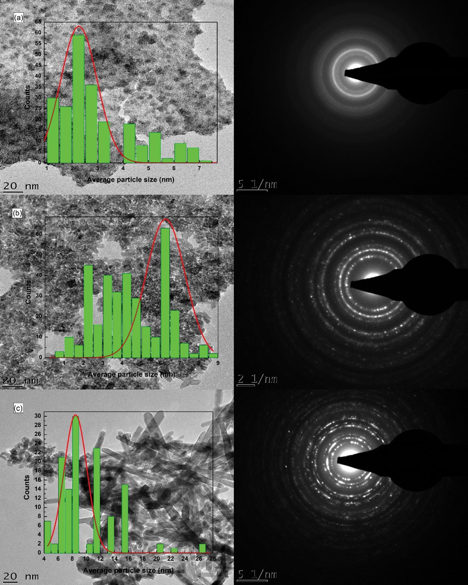
Volume 120| Number 3/4 March/April 2024 102 https://doi.org/10.17159/sajs.2024/16026 Research Article Unsupported IrO2 nano-catalysts for PEMWE Page 4 of 9
Figure 3: HRTEM and corresponding SAED analyses of the IrO2 synthesised with the MSM at temperatures (a) 350 °C, (b) 500 °C and (c) 650 °C.
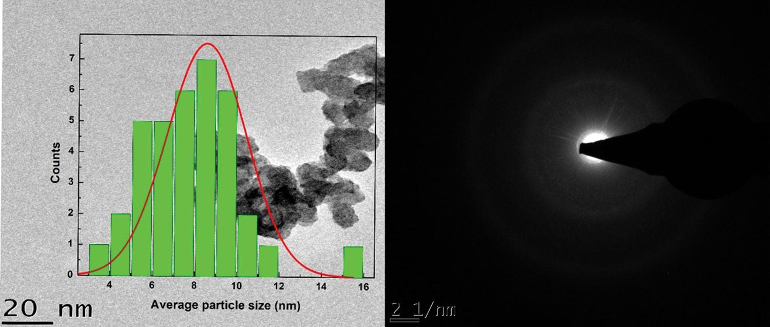
MAFM-350 2.732.31216.23
MAFM-500 7.783.54104.84
MAFM-650 10.01Width: 5.2353.84
Length: 11.36
MSM-350 2.834.1263.89
MSM-500 7.054.7455.62
MSM-650 12.43Width: 2.7331.77
Length: 26.36
Electrochemical characterisation
The cyclic voltammograms were obtained in a potential window of 0 and +1.4 V versus RHE with a potential scan rate of 20 mVs−1. The cyclic voltammograms seem to be influenced by the synthesis temperatures since there is a slight shift in the two redox couples, Ir(III)/Ir(IV) and Ir(IV)/Ir(V), as shown in Table 2. IrO2 catalysts typically display a lowering in current density and charge as the synthesis temperatures are increased.7,22,26 Heat treatment is known to dehydrate and crystallise the IrO2 material, thereby reducing the utilisation of Ir atoms participating in reactions to as low as 1%–2%.(7) In Figure 5a, the Ir(III)/Ir(IV) and Ir(IV)/Ir(V) redox couples for MAFM-350, MAFM-500 and MAFM-650 were observed. Between 0 and +0.65 V versus RHE, no charges were transferred for the MAFM-500 and MAFM-650 due to double-layer charging.22 In Figure 5b, the Ir(III)/Ir(IV) and Ir(IV)/Ir(V) redox couples for the MSM-350, MSM-500 and MSM-650 were observed, and the peak potentials are also summarised in Table 2. For the anodic potential scan, an additional pre-peak was seen at +0.35 and +0.59 V versus RHE for MAFM-350 and MSM-350, respectively. The peak can also be seen for the commercial IrO2. The cause of the peaks may be due to the coupled ion-electron transfer, formal potential distribution, relations in the layer or the change in mass transport within the layer as the potential change.22,27 The pre-peak is also believed to occur due to the oxidation of Ir3+ close to the metal/oxide interface and is accompanied by extensive water exchange.7 IrO2 synthesised at 500 °C and 650 °C does not exhibit these pre-peaks, ruling out the oxidation/reduction of a sodium layer impurity and also confirming the formation of a dehydrated IrO2 material due to a lack of the water exchange that takes place during the pre-peak formation. Therefore, the additional peaks are almost certainly
due to the presence of active Ir(III) sites at slightly shifted oxidising/ reducing potentials. Additionally, the incomplete decomposition of the Ir-metal precursor in the oxide phase may also show the presence of active sites.28 Upon the cathodic potential scan at 0 V versus RHE, a strong negative ‘tail’ was seen for MAFM-500, MAFM-650, MSM500 and MSM-650. This reflects their negative capacitive behaviour (Hads), involving the double-layer and pseudo- capacitances.22,28 These CV-shaped curves are like those found by Rasten et al.26, especially for the IrO2 synthesised at increased synthesis temperatures.
The polarisation curves were obtained using the LSV technique that was performed between +0.8 and +1.8 V versus RHE at a potential scan rate of 2 mVs−1. It is commonly understood that amorphous IrO2 displays higher OER activity due to complete IrO2 atom utilisation but suffers stability due to being prone to dissolution. In contrast, crystalline IrO2 lacks the activity due to low IrO2 atom utilisation and change in oxide stoichiometry towards the crystalline phase, but displays higher stability.29 Thus, a strong relationship exists between the structural properties and electrocatalytic performance due to the presence of a mixture of amorphous and crystalline IrO2 29 The polarisation curves of the IrO2 synthesised with the MAFM and MSM are shown in Figure 6a and 6c, respectively. The OER onset potentials of the synthesised IrO2 were found to be at 1.5 V versus RHE due to the energy requirement during the H2O phase transition.30 MSM-350 had the lowest overpotential of 270 mV compared to 280 mV for MAFM-350. For MAFM, peak OER activity for IrO2 was observed at 500 °C, which is contrary to findings in the literature, which suggest that the amorphous IrO2 would be more active. For MSM, the lowest overpotential was observed for MSM350. At lower current densities (10 mAcm−2), the MAFM-350 and MSM-350 had higher OER activities. However, at increased current densities (150 mAcm−2), the MAFM-500 and MSM-500 had higher OER activities. There were no results generated at 150 mAcm−2 for MAFM-650 due to the IrO2 degradation caused by the Ir dissolution.31 The performance difference between MAFM-650 and MSM-650 is quite notable, and the explanation is not clear as MAFM-650 had a higher BET surface and a similar CV to MSM-650. A possible explanation could be due to structural defects occurring during the formation of the Ir5+ surface where the OER takes place, which could also explain the higher overpotential at 10 mAcm−2. Surface reconstruction occurs during the OER process to expose the real active species while the pristine catalyst could be considered pre-catalysts.32 Different crystallinity induced by the synthesis temperature typically affects the dissolution rates of IrO2 with higher stability and lower activities being the result of higher temperatures. Rasten et al.26 also show improved OER activity of IrO2 synthesised at decreased temperatures. Most anodically produced IrO2 electrodes have a corresponding Tafel slope of about 44 mV dec−1 5,13 Figure 6b and 6d show the Tafel slopes of the IrO2 catalysts synthesised via the MAFM and MSM, respectively. For both synthesis methods, IrO2 synthesised at 350 °C exhibited the smallest Tafel slopes, i.e. 62.41 mV dec−1 for MAFM-350 and 59.17 mV dec−1 for MSM-350, while the Tafel slope magnitude increased with higher synthesis temperatures. IrO2 catalyst with a smaller Tafel slope generates current more efficiently
Volume 120| Number 3/4 March/April 2024 103 https://doi.org/10.17159/sajs.2024/16026 Research Article Unsupported IrO2 nano-catalysts for PEMWE Page 5 of 9
Sample name XrD crystallite/ particle sizes (nm) hrtEM particle sizes (nm) BEt surface area (m2/g)
Figure 4: HRTEM and corresponding SAED analyses of the commercial IrO2
Commercial Iro2
–8.6925.11
table 1: Physical characterisation properties of the commercial, MAFM and MSM IrO2 catalysts
Unsupported IrO2 nano-catalysts for PEMWE
Research Article
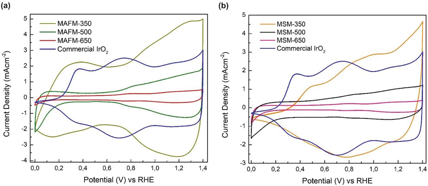
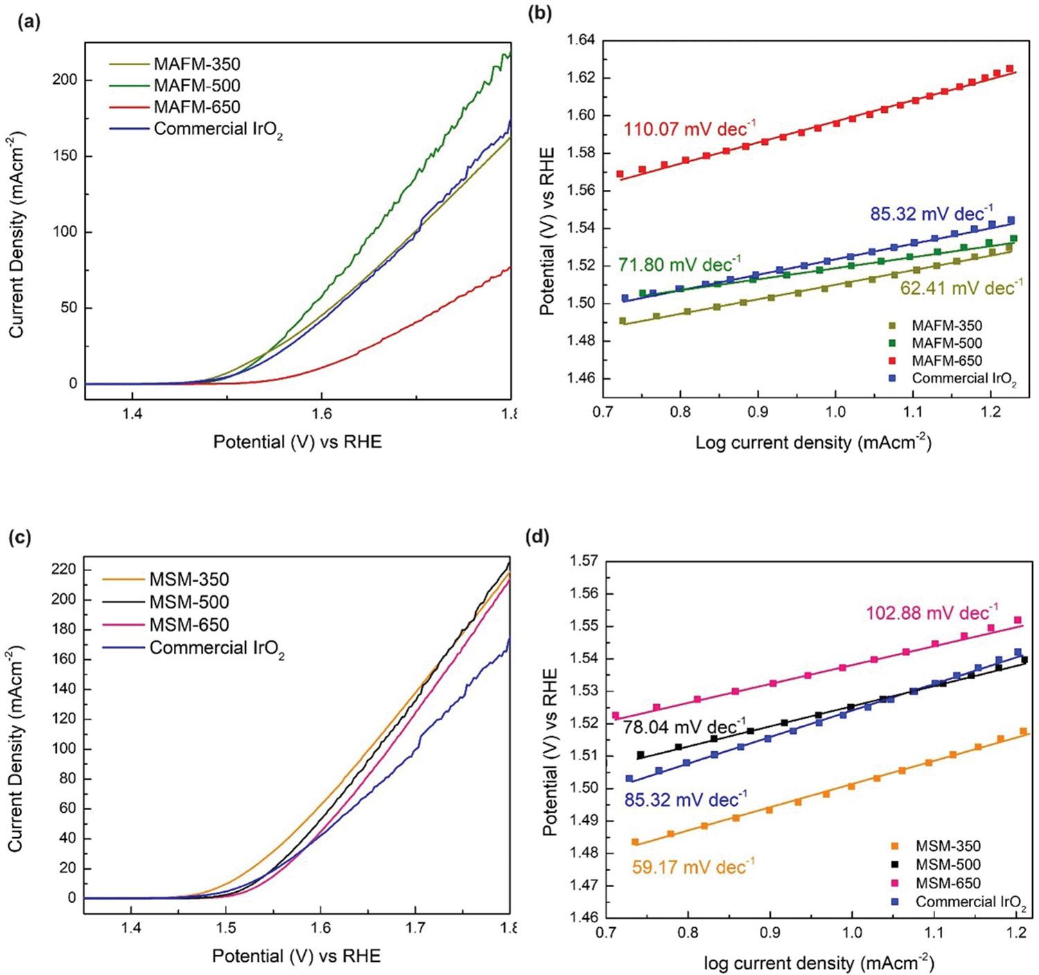
Volume 120| Number 3/4 March/April 2024 104 https://doi.org/10.17159/sajs.2024/16026
Page 6 of 9
Sample name Ir(III)/Ir(IV) anodic redox couple (V vs. rhE)
Ir(IV)/Ir(V)
MAFM-350 +0.94 +0.43 +1.30 +0.92 MAFM-500 +0.82 +0.76 +1.28 +1.15 MAFM-650 +0.78 +0.77 +1.18 +1.18 MSM-350 +0.97 +0.79 +1.20 +0.98 MSM-500 +0.80 +0.81 +1.23 +1.09 MSM-650 +0.65 +0.82 +1.17 +1.16 Commercial Iro2 +0.74 +0.75 +1.16 +1.15
Ir(III)/Ir(IV) cathodic redox couple (V vs. rhE) Ir(IV)/Ir(V) anodic redox couple (V vs. rhE)
cathodic redox couple (V vs. rhE)
table 2: Anodic/cathodic peak potentials of the Ir(III)/Ir(IV) and Ir(IV)/Ir(V) redox couples of the commercial, MAFM and MSM IrO2 catalysts
Figure 6: (a) LSV analysis at 2 mVs−1 in 0.5M H2SO4 of the commercial IrO2 and MAFM IrO2 catalysts, (b) Tafel plots of the commercial IrO2 and MAFM IrO2 catalysts, (c) LSV analysis at 2 mVs−1 in 0.5M H2SO4 of the commercial IrO2 and MSM IrO2 catalysts and (d) Tafel plots of the commercial IrO2 and MSM IrO2 catalysts.
Figure 5: CV analysis at 20 mVs−1 in 0.5M H2SO4 of the commercial IrO2 and IrO2 synthesised with the (a) MAFM and (b) MSM.
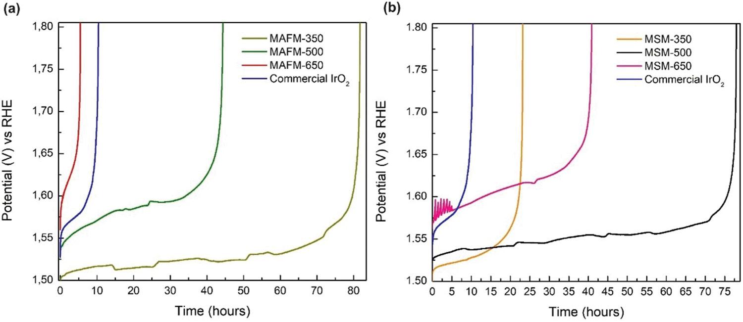
when voltage is applied.13,14 Siracusano et al.19 synthesised IrO2 catalysts with an overall Tafel slopes of 80 mV dec−1. The Tafel slope consisted of an anodic contribution of 59.17 mV dec−1 and a cathodic contribution due to the OH adsorbed intermediates. Dang et al. developed a 1-T phase IrO2 with an overpotential of 235 mV and a Tafel slope of 49 mV dec−1; however, the synthesis method was highly challenging.33 Table 3 summarises the electrochemical properties of the IrO2 catalysts. The catalyst mass activities were determined at 1.6 V versus RHE. For the MAFM, MAFM-500 had the highest mass activity (137 Ag−1), whereas for the MSM, MSM-350 had the highest mass activity (140 Ag−1). The commercial IrO2 catalyst exhibited a mass activity of (101 Ag−1). For the MSM, there was a decreasing activity trend with the increase in synthesis temperature, while for the MAFM, peak activity was observed at a synthesis temperature of 500 °C. Higher mass activities may be attributed to catalyst nanostructures, which allow more exposure to the active sites.4 The commercial IrO2 had a lower OER activity when compared to the synthesised IrO2 from both the MAFM and MSM. The lower OER activities of MAFM-650, MSM-650 and commercial IrO2 can be attributed to the larger crystallite/particle sizes shown by the XRD and HRTEM analyses.
CP analysis was performed at 10 mAcm−2 until the potential reached a value of 1.8 V versus RHE. Performance degradation is normally attributed to dissolution of the IrO2 catalyst.34 Figure 7a shows the CP analysis of the IrO2 synthesised with the MAFM. MAFM-350 had the highest OER stability of 82 h before reaching the cut-off potential. MAFM-500 and MAFM-650 were stable for ~44 h and ~5 h, respectively. Figure 7b shows the IrO2 synthesised with the MSM. MSM-500 had the highest OER stability of 75 h. The stability of MSM-500 was on par with the stability of MAFM-350. MSM-650 was stable for 41 h compared to 23 h for MSM-350. The low stability of MSM-350 appears to be the result of the formation of a highly amorphous IrO2, which lacks the stable facets of IrO2 needed for stable OER performance. The stability
of MSM-350 is more in line with the expected stability of an amorphous IrO2 catalyst compared to crystalline IrO2 catalysts. However, MAFM350 showed stability that exceeded the stability of its more crystalline IrO2 counterparts, which is contrary to what is commonly expected from amorphous IrO2 catalysts. The high stability of MAFM-350 could be due to more active sites (deduced from high BET surface area) available for the OER. The detachment of bubble formation on MAFM-350 at an early stage of the analyses may have also contributed to the increased stability.35 The commercial IrO2 was stable for ~10 h, outperforming only MAFM-650. A possible explanation for the poor performance of MAFM-650 could be due to structural defects during formation of the Ir5+ oxidation state where the OER takes.35 The low stability of the commercial IrO2 could be due to both physical and chemical properties such as low surface area and the presence of metallic Ir. Banti et al.29 also observed a lower BET surface area and OER performance for this commercial IrO2 catalyst compared to their synthesised IrO2 catalysts. A summary of the catalysts’ stabilities is provided in Table 3.
Conclusion
IrO2 catalysts suitable for the OER in PEMWE were successfully produced using MAFM and MSM. Both methods can be easily scaled for high-volume metal oxide production. The effects of synthesis method and temperature on the OER performance of the IrO2 catalysts were studied. It was found that MAFM and MSM influenced the OER performance of the IrO2 catalysts. However, no specific synthesis method showed both increased OER activity and stability. The effect of temperature on the IrO2 catalyst performance was different for the two synthesis methods. At 350 °C, the two methods yielded IrO2 catalysts with contrasting OER performance, i.e. MAFM-350 had significantly better stability but lower activity compared to MSM-350. At 500 °C, MAFM-500 and MSM-500 had similar activities; however, MSM-500 had significantly better stability. At 650 °C, MSM-650 had better activity and stability compared to MAFM-650 with MSM-650 having the poorest overall OER activity of all the IrO2 catalysts studied. The
Volume 120| Number 3/4 March/April 2024 105 https://doi.org/10.17159/sajs.2024/16026 Research Article Unsupported IrO2 nano-catalysts for PEMWE Page 7 of 9
Sample name overpotential at 10 mAcm−2 (mV vs. rhE) tafel slopes (mV dec−1) Mass activity at 1.6 V vs. rhE (Ag−1) Potential
vs. rhE) Stability
MAFM-350 27962.411031.79c82 MAFM-500 29271.801371.7244 MAFM-650 359110.0728–5 MSM-350 27159.171401.7223 MSM-500 29978.041221.7175 MSM-650 311102.881031.7341 Commercial Iro2 29185.321011.7710
at 150 mAcm−2 (V
at 10 mAcm−2 (hours)
table 3: Electrochemical properties of the commercial, MAFM and MSM IrO2 catalysts
Figure 7: CP analysis at 10 mAcm−2 in 0.5M H2SO4 of the commercial IrO2 and IrO2 synthesised with the (a) MAFM and (b) MSM.
commercial IrO2 exhibited expected performance trends where amorphous IrO2 has good activity but low stability. The XRD analysis showed a phase transition, from amorphous to crystalline, as the synthesis temperature was increased from 350 °C to 650 °C. IrO2 catalysts synthesised at 350 °C were spherical shaped and amorphous. Above 500 °C synthesis temperatures, the IrO2 catalysts synthesised via MAFM had cubic and cylindrical shapes, whereas the IrO2 catalysts synthesised via MSM consisted of crystallites with different shapes. This study demonstrates that the physical properties of the IrO2 catalysts can be tailored through the synthesis method and the synthesis conditions, which can result in significant improvements in the OER performance of the IrO2 catalysts. Improved catalyst OER performance is essential to lower the catalyst loading requirements, which will in turn lower the costs associated with the catalyst component.
Acknowledgements
This work was funded by the Technology and Human Resources for Industry Programme (THRIP/19/31/08/2018) under the Department of Trade, Industry and Competition of the Republic of South Africa. We thank the anonymous reviewers for their valuable comments that improved this article.
Competing interests
We have no competing interests to declare.
Authors’ contributions
S.K.: Data curation, investigation, formal analysis, conceptualisation, methodology, writing – original draft, writing – revisions and editing. C.F.: Visualisation, conceptualisation, methodology, formal analysis, writing –revisions and editing. S.P.: Visualisation, funding acquisition, project administration, supervision.
references
1. International Renewable Energy Agency (IRENA). Green hydrogen cost reduction. Abu Dhabi: IRENA; 2020. p. 105.
2. Chen Z, Duan X, Wei W, Wang S, Ni BJ. Electrocatalysts for acidic oxygen evolution reaction: Achievements and perspectives. Nano Energy. 2020;78, Art. #105392. https://doi.org/10.1016/j.nanoen.2020.105392
3. Yu J, Dai Y, He Q, Zhao D, Shao Z, Ni M. A mini-review of noble-metal-free electrocatalystsforoverallwatersplittinginnon-alkalineelectrolytes.MaterReports Energy. 2021;1(2), Art. #100024. https://doi.org/10.1016/j.matre.2021.100024
4. Liu Y, Liang X, Gu L, Zhang Y, Li GD, Zou X. Corrosion engineering towards efficient oxygen evolution electrodes with stable catalytic activity for over 6000 hours. Nat Commun. 2018;9(1):1–10. https://dx.doi.org/10.1038/s4 1467-018-05019-5
5. TouniA,GrammenosOA,BantiA,KarfaridisD,ProchaskaC,LambropoulouD. Iridium oxide-nickel-coated titanium anodes for the oxygen evolution reaction. Electrochim Acta. 2021;390, Art. #138866. https://doi.org/10.1016/j.electa cta.2021.138866
6. Wang T, Cao X, Jiao L. PEM water electrolysis for hydrogen production: Fundamentals, advances, and prospects. Carbon Neutrality. 2022;1(1):1–19. https://doi.org/10.1007/s43979-022-00022-8
7. Geiger S, Kasian O, Shrestha BR, Mingers AM, Mayrhofer KJJ, Cherevko S. Activity and stability of electrochemically and thermally treated iridium for the oxygen evolution reaction. J Electrochem Soc. 2016;163(11):F3132–F3138. https://doi.org/10.1149/2.0181611jes
8. Gupta SK, Mao Y. A review on molten salt synthesis of metal oxide nanomaterials: Status, opportunity, and challenge. Prog Mater Sci. 2021;117, Art. #100734. https://doi.org/10.1016/j.pmatsci.2020.100734
9. Adams R, Shriner R. Platinum oxide as a catalyst in the reduction of organic compounds III: Preparation and properties of the oxide of platinum obtained by the fusion of chloroplatinic acid with sodium nitrate. J Am Chem Soc. 1923;9:2171–2179. https://doi.org/10.1021/ja01662a022
10. Liu Y, Wang C, Lei Y, Liu F, Tian B, Wang J. Investigation of high-performance IrO2 electrocatalysts prepared by Adams method. Int J Hydrogen Energy. 2018;43(42):19460–19467. https://doi.org/10.1016/j.ijhydene.2018.08.196
11. Jorge AB, Dedigama I, Miller TS, Shearing P, Brett DJL, McMillan PF. Carbon nitride materials as efficient catalyst supports for proton exchange membrane water electrolyzers. Nanomaterials. 2018;8(6), Art. #432. https://doi.org/1 0.3390/nano8060432
12. Baik C, Lee SW, Pak C. Glycine-induced ultrahigh-surface-area IrO2@IrOx catalyst with balanced activity and stability for efficient water splitting. Electrochim Acta. 2021;390, Art. #138885. https://doi.org/10.1016/j.elect acta.2021.138885
13. Cheng J, Zhang H, Ma H, Zhong H, Zou Y. Preparation of Ir0.4Ru0.6MoxOy for oxygen evolution by modified Adams’ fusion method. Int J Hydrogen Energy. 2009;34(16):6609–6613. http://dx.doi.org/10.1016/j.ijhydene.2009.06.061
14. Lim J, Kang G, Lee JW, Jeon SS, Jeon H, Kang PW, et al. Amorphous Ir atomic clusters anchored on crystalline IrO2 nanoneedles for proton exchange membrane water oxidation. J Power Sources. 2022;524, Art. #231069. http s://doi.org/10.1016/j.jpowsour.2022.231069
15. Yuasa M. Molten salt synthesis of Nb-doped TiO2 rod-like particles for use in bifunctional oxygen reduction/evolution electrodes. Ceram Int. 2022;48(10): 14726–14735. https://doi.org/10.1016/j.ceramint.2022.02.009
16. Ahmed J, Mao Y. Ultrafine iridium oxide nanorods synthesized by molten salt method toward electrocatalytic oxygen and hydrogen evolution reactions. Electrochim Acta. 2016;212:686–693. https://dx.doi.org/10.1016/j.electacta. 2016.06.122
17. Carmo M, Fritz DL, Mergel J, Stolten D. A comprehensive review on PEM water electrolysis. Int J Hydrogen Energy. 2013;38(12):4901–4934. https:// doi.org/10.1016/j.ijhydene.2013.01.151
18. Puthiyapura VK, Pasupathi S, Basu S, Wu X, Su H, Varagunapandiyan N. RuxNb1-xO2 catalyst for the oxygen evolution reaction in proton exchange membrane water electrolysers. Int J Hydrogen Energy. 2013;38(21):8605–8616. https://doi.org/10.1016/j.ijhydene.2013.04.100
19. Siracusano S, Baglio V, Di Blasi A, Briguglio N, Stassi A, Ornelas R. ElectrochemicalcharacterizationofsinglecellandshortstackPEMelectrolyzers based on a nanosized IrO2 anode electrocatalyst. Int J Hydrogen Energy. 2010;35(11):5558–5568. https://dx.doi.org/10.1016/j.ijhydene.2010.03.102
20. Aricò AS, Siracusano S, Briguglio N, Baglio V, Di Blasi A, Antonucci V. Polymer electrolyte membrane water electrolysis: Status of technologies and potential applications in combination with renewable power sources. J Appl Electrochem. 2013;43(2):107–118. https://doi.org/10.1007/s10800-012-0490-5
21. Hu JM, Meng HM, Zhang JQ, Cao CN. Degradation mechanism of long service life Ti/IrO2-Ta2O5 oxide anodes in sulphuric acid. Corros Sci. 2002;44(8):1655–1668. https://doi.org/10.1016/S0010-938X(01)00165-2
22. Felix C, Bladergroen BJ, Linkov V, Pollet BG, Pasupathi S. Ex-situ electrochemical characterization of IrO2 synthesized by a modified Adams fusion method for the oxygen evolution reaction. Catalysts. 2019;9(4), Art. #318. https://doi.org/10.3390/catal9040318
23. Zhang Y, Wang C, Mao Z, Wang N. Preparation of nanometer-sized SnO2 by the fusion method. Mater Lett. 2007;61(4–5):1205–1209. https://doi.org/10 .1016/j.matlet.2006.06.083
24. SubramanianV,HallSC,SmithPH,RambabuB.MesoporousanhydrousRuO2 as a supercapacitor electrode material. Solid State Ion. 2004;175(1–4):511–515. https://doi.org/10.1016/j.ssi.2004.01.070
25. Ma Z, Zhang Y, Liu S, Xu W, Wu L, Hsieh YC, et al. Reaction mechanism for oxygen evolution on RuO2, IrO2, and RuO2@IrO2 core-shell nanocatalysts. J Electroanal Chem. 2018;819:296–305. https://doi.org/10.1016/j.jelechem .2017.10.062
26. Rasten E, Hagen G, Tunold R. Electrocatalysis in water electrolysis with solid polymer electrolyte. Electrochim Acta. 2003;48(25–26):3945–3952. https:// doi.org/10.1016/j.electacta.2003.04.001
27. Steegstra P, Busch M, Panas I, Ahlberg E. Revisiting the redox properties of hydrous iridium oxide films in the context of oxygen evolution. J Phys Chem. 2013;117:20975–20981. https://doi.org/10.1021/jp407030
28. Grupioni AAF, Arashiro E, Lassali TAF. Voltammetric characterization of an iridiumoxide-basedsystem:ThepseudocapacitivenatureoftheIr0.3Mn0.7O2 electrode. Electrochim Acta. 2002;48(4):407–418. https://doi.org/10.1016/ S0013-4686(02)00686-2
Volume 120| Number 3/4 March/April 2024 106 https://doi.org/10.17159/sajs.2024/16026 Research Article Unsupported IrO2 nano-catalysts for PEMWE Page 8 of 9
29. Banti A, Papazisi KM, Balomenou S, Tsiplakides D. Effect of calcination temperature on the activity of unsupported IrO2 electrocatalysts for the oxygen evolution reaction in polymer electrolyte membrane water electrolyzers. Molecules. 2023;28(15), Art. #5827. https://doi.org/10.3390/molecules2815 5827
30. HanSB,MoYH,LeeYS,LeeSG,ParkDH,ParkKW.Mesoporousiridiumoxide/ Sb-doped SnO2 nanostructured electrodes for polymer electrolyte membrane water electrolysis. Int J Hydrogen Energy. 2020;45(3):1409–1416. https://d oi.org/10.1016/j.ijhydene.2019.11.109
31. Feng Q, Yuan XZ, Liu G, Wei B, Zhang Z, Li H. A review of proton exchange membrane water electrolysis on degradation mechanisms and mitigation strategies. J Power Sources. 2017;366:33–55. https://doi.org/10.1016/j.jp owsour.2017.09.006
32. Chen S, Ma L, Huang Z, Liang G, Zhi C. In situ/operando analysis of surface reconstruction of transition metal-based oxygen evolution electrocatalysts. Cell Reports Phys Sci. 2022;3(1), Art. #100729. https://doi.org/10.1016/ j.xcrp.2021.100729
33. Dang Q, Lin H, Fan Z, Ma L, Shao Q, Ji Y, et al. Iridium metallene oxide for acidic oxygen evolution catalysis. Nat Commun. 2021;12(1), Art. #6007. https://doi.org/10.1038/s41467-021-26336-2
34. Ouattara L, Fierro S, Frey O, Koudelka M, Comninellis C. Electrochemical comparison of IrO2 prepared by anodic oxidation of pure iridium and IrO2 prepared by thermal decomposition of H2IrCl6 precursor solution. J Appl Electrochem. 2009;39(8):1361–1367. https://doi.org/10.1007/s10800-00 9-9809-2
35. Spöri C, Kwan JTH, Bonakdarpour A, Wilkinson DP, Strasser P. The stability challenges of oxygen evolving catalysts: Towards a common fundamental understanding and mitigation of catalyst degradation. Angew Chemie Int Ed. 2017;56(22):5994–6021. https://doi.org/10.1002/anie.201608601
Volume 120| Number 3/4 March/April 2024 107 https://doi.org/10.17159/sajs.2024/16026 Research Article Unsupported IrO2 nano-catalysts for PEMWE Page 9 of 9
AuthorS:
Kingsley O. Omeje1
Benjamin O. Ezema2,3,4
Sabinus O.O. Eze1
AFFILIAtIoNS:
1Department of Biochemistry, University of Nigeria, Nsukka, Nigeria
2The Biochemistry Unit, Department of Science Laboratory Technology, University of Nigeria, Nsukka, Nigeria
3Aston Institute of Materials Research, Aston University, Birmingham, UK
4Energy and Bioproducts Research Institute, Aston University, Birmingham, UK
CorrESPoNDENCE to:
Benjamin Ezema
EMAIL:
ezema.onyebuchi@unn.edu.ng
DAtES:
received: 17 Apr. 2023
revised: 28 Oct. 2023
Accepted: 06 Nov. 2023
Published: 27 Mar. 2024
hoW to CItE:
Omeje KO, Ezema BO, Eze SOO. Evaluation of pesticide residues and heavy metals in common food tubers from Nigeria. S Afr J Sci. 2024;120(3/4), Art. #15969. https:// doi.org/10.17159/sajs.2024/15969
ArtICLE INCLuDES:
☒ Peer review
☒ Supplementary material
DAtA AVAILABILItY:
☐ Open data set
☒ All data included
☐ On request from author(s)
☐ Not available
☐ Not applicable
EDItor:
Priscilla Baker
KEYWorDS:
tubers, pesticide residue analysis, heavy metal analysis, gas chromatography–mass spectrometry, atomic absorption spectroscopy, maximum permissible limit
FuNDING:
None
Research Article
Evaluation of pesticide residues and heavy metals in common food tubers from Nigeria
Pesticide residues and heavy metal content of cassava, yam, cocoyam, potato, water yam and carrot were evaluated by gas chromatography–mass spectrometry and atomic absorption spectroscopy. The detected pesticide residues in the samples were 2,4-dichlorophenoxyacetic acid, glyphosate, hexachlorobenzene (HCB), dichlorobiphenyl, aldrin, endosulfan, profenofos, g-chlordane, carbofuran, biphenyl, heptachlor, lindane and t-Nonachlor. The concentration of HCB ranged between 0.0799 ± 0.06 mg/kg and 0.1596 ± 0.00 mg/kg, which was greater than the permitted maximum limit of 0.5 mg/kg established by the US Environmental Protection Agency. The concentration of aldrin and profenofos detected was lower than the predetermined maximum allowed limits. Endosulfan concentrations in cocoyam (0.2500 mg/kg) and potato (0.3265 mg/kg) were higher than the limits allowed by the Canadian Department of Industrial Research. The heavy metals detected in these samples include cobalt, nickel, lead, manganese, chromium, arsenic and mercury in at least one of the samples evaluated. There was not much difference between the concentration of cobalt in yam (0.036 mg/kg) and the maximum allowed concentration (0.043 mg/kg). Lead was detected in potatoes and carrots but was below detectable concentration in cassava, yam, cocoyam and water yam. Similarly, cocoyam was found to have a significant mercury content (0.658 mg/kg), but mercury content was below detectable concentrations in cassava, yam and water yam.
Significance:
Heavy metal pollutants and pesticide residues can impair human health, and their presence in food can cause various illnesses and health issues. It is important to prevent exposure to these contaminants and ensure that food is safe by identifying and monitoring them. Farmers may provide consumers with more assurance that their products are safe by identifying and monitoring pesticide residues and heavy metal contamination in these food crops. Overall, it is crucial to find and monitor pesticide residues and heavy metal contamination in food to safeguard customer confidence, ensure legal compliance and preserve human health.
Introduction
Pesticides are chemicals that are used to control pests which are harmful to humans, plants and the environment.1 In parallel, pesticide residues are described as substances that are found in foods for consumption by humans or other animals, and are chemical derivatives considered to be toxic to living organisms.2 Similar to pesticide residues, the entrance of heavy metals into the food chain is their major route into the human system, which could cause autoimmune disorders and inhibit the functions of some biochemical processes.3 Heavy metal toxicity has been reported regularly in recent times, with some deaths attributed to it. Other effects of heavy metals on humans include cancers, high blood pressure and gene mutation.2,4,5 Uncontrolled disposal of household and electronic waste, animal dung and abandoned metallic parts are some of the environmental sources of heavy metals.6 Environmental pollution is a serious problem in today’s modern world, with pesticides and heavy metal pollution being the most prevalent due to their ability to contaminate air and water.7
Cassava, yam, cocoyam, potato, water yam and carrot are commonly cultivated in Nigeria due to their multiple usage and nutritional values. These tubers are tropical crops consumed by about 2 billion people and are the major sources of carbohydrates providing energy for the roughly 700 million residents of tropical and subtropical regions.8 The production of these products and their conversion into goods derived from food is expanding, and farmers profit significantly from their market.8 Their high post-harvest losses, due to contamination by external and internal hazardous substances (such as mycotoxins, heavy metals and insecticides), reduce economic value and income. These roots/tubers have a crude fat content on the fresh weight of 0.1–0.5% and 1–3% on the dry weight, of which 80% is starch. The carbohydrate content of cassava is larger than that of potatoes.8 Cassava is a potent source of energy despite being deficient in lipids, minerals and proteins.9 On the other hand, yam provides energy in the range of 80–120 kcal/100 g.10 Vitamin A is produced from beta-carotene, and it is present in adequate amounts in potatoes.11 These tubers’ essential amino acid composition is higher than that recommended by the Food and Agriculture Organization (FAO) for daily protein intake and greater than that of soybean protein.12 These tubers may become polluted during cultivation and food processing and also contain certain endogenous antinutrients.
Currently, there are common applications of several agrochemicals in the cultivation of these crops to ward off pests. All the grown food crops are highly vulnerable to various insect attacks, especially on the farm or in the cultivation area, which has a detrimental impact on both the financial and dietary elements of product quality. Pesticides must be used to control pest infestations, which helps to improve the quality of crops and their production on farms.13 Consequently, these tubers may get contaminated, and the risks associated with consuming these roots can be divided into two groups: those related to potentially harmful substances present in the crop itself, and those related to processing and product development. However, there are some significant concerns regarding food safety and security. A lot of research still needs to be carried out concerning the level of heavy metal
108 https://doi.org/10.17159/sajs.2024/15969 Volume 120| Number 3/4 March/April 2024 © 2024. The Author(s). Published under a Creative Commons Attribution Licence.
and pesticide pollution, especially that seen in Nigerian food crops like the tubers that are commonly consumed, such as cassava, yam and cocoyam.14,15
The amount of residues from pesticides and heavy metals in tuberderived food products varies based on the location of the growing area and the system of farming. In Nigeria, pesticide residues detected in some tubers (cassava and yam) were HCB (0.0247), endosulfan (0.0340 and 0.090) and aldrin (0.0000 and 0.0937) mg/kg, respectively.15 The concentration of isopropylamine in yam was 0.2165 ± 0.00 mg/kg and in cassava was 0.1649 ± 0.00 mg/kg, while the concentration of t-Nonachlor in yam was 0.1093 ± 0.00 mg/kg and in cassava was 0.0006 ± 0.00 mg/kg, as reported by Omeje et al.15 Adeyeye and Osibanjo16 detected high concentrations of organochlorine residues in yam (aldrin = ~5.0 µg/kg; dieldrin = ~24.0 µg/kg and p,p´-DDE = ~13.0 µg/kg) and cassava (aldrin = ~6.0 µg/kg; dieldrin = ~31.0 µg/ kg and p,p´-DDE = ~21.0 µg/kg) in their study. Heavy metals have been found in tubers like potatoes, yams and cassava in previous studies. The amount of cadmium (Cd) found in yam was reported to be 0.11 mg/kg, and lead (Pb) and nickel (Ni) were also detected.17 In addition, 0.21 mg/ kg of Pb, 42 mg/kg of copper (Cu), 24 mg/kg of zinc (Zn), 18 mg/kg of manganese (Mn) and 12 mg/kg of Ni were reported by Wilberforce and Nwabue18. Arsenic (As) concentration in cassava was detected to be 0.017 mg/kg.15 According to Onianwa et al.19, the range reported for Ni concentrations in tubers is 0.93–1.79 mg/kg. Akinyele and Shokunbi20 detected Mn in yams (~4.42 mg/kg), and Orisakwe et al.21 reported Pb (~0.33 mg/kg), Cd (~0.10 mg/kg) and Ni (~0.30 mg/kg) in cassava.
To enrich the existing body of information, we assessed the presence and concentration of common food pesticide residues and heavy metal contaminants in essential and commonly consumed tuber crops cultivated in Nigeria using gas chromatography–mass spectrometry (GC–MS) and atomic absorption spectroscopy.
Materials and methods
Chemicals and materials
The chemicals and reagents used were of analytical quality and included chloroform, perchloric acid, sodium sulfate, concentrated sulfuric acid (Sigma-Aldrich), n-hexane (Loba Chemie, India) and concentrated nitric acid, anhydrous sodium sulfate, methanol (Sigma-Aldrich) and benzene. The pesticide standards (purity > 95%) were obtained from Restek (Sigma-Aldrich, USA). With concentrations ranging from 50 ng/mL to 200 ng/mL, stock standard solutions of 47 organochlorine pesticides (OCPs), organophosphorus pesticides (OPPs) and other pesticides were made in ethyl acetate and stored at 4 °C in a dark location until analysis. Pesticides are present in spiking solutions in amounts of 10–50 ng/L. The internal standard was aldrin solution (Sigma-Aldrich) in acetone at a concentration of 50 ng/L.
Samples
In April 2022, fresh tubers weighing 500 g each (cassava, yam, cocoyam, potato, water yam and carrot) were purchased from Nsukka open market situated in Enugu State (6°51’24” N and 7°23’45” E) in southeast Nigeria, and transported to the laboratory of the Department of Biochemistry, University of Nigeria, Nsukka. They were processed and stored at 4 °C for further analysis.
Pesticide residue analysis
The pesticide residues were determined with the help of a GC analysis and prepared following the AOAC method22, with minor modifications. Ten grams (10 g) of the homogenised sample was mixed with 60 g of anhydrous sodium sulfate in an agate mortar to absorb moisture. The homogenate was transferred into a 500 mL beaker, and the extraction was carried out with 300 mL of n–hexane for 24 h. The obtained crude extract was concentrated using a rotary vacuum evaporator at 40 °C to dryness. The sample residue (1 mL) was measured into 50 mL of chloroform transferred to a 100 mL volumetric flask and diluted. Most of the chloroform was evaporated at room temperature before adding 1 mL of the solvent mixture (20% benzene and 55% methanol). The mixture
was sealed and heated at 40 °C using a water bath for 10 min. After heating, the organic sample was extracted with n–hexane and water in a proportion of 1:1. The mixture was shaken vigorously for 2 min, and n-hexane phase was transferred onto a small test tube for injection into a Buck 530 Gas Chromatograph (GC) equipped with an on-column, automatic injector, electron capture detector and an HP 88 capillary column (100 mm X 0.25 µm film thickness) (Agilent Technologies, Santa Clara, CA, USA), with injector and detector temperatures of 180 °C and 300 °C, respectively. Overall, the GC enabled the identification of pesticide residues, which were recorded in mg/kg, as the results emerged.
Heavy metal analysis
The heavy metal analysis (Co, Ni, Pb, Mn, Cr, As, Hg and Cd) was performed using a Varian AA240 Atomic Absorption Spectrophotometer (AAS; Varian Inc., Palo Alto, CA, USA) equipped with an acetylene air flame, adapting the protocol described by Quarcoo and Adotey23, with slight modifications. The pyrolytic-coated graphite tubes of the AAS were equipped with platform instrument settings and furnace programs that helped to ascertain the peak signals. A known concentration of the sample (~2 g) was put into a digestion flask, along with 20 mL of acid mixture (which consisted of 650 mL concentrated HNO3; 80 mL perchloric acid; 20 mL concentrated H2SO4), and subsequently heated until a clear digest was obtained. The digest was diluted with distilled water to the 100 mL mark. The acid level samples as they came along were monitored by a pH meter. The digestate was quantified, assayed for heavy metals using a Varian AA240 Spectrophotometer, and reported in mg/kg. The reference standards (Fluka Analytical, Sigma-Aldrich Chemie GmbH, Switzerland) for the detected element, blanks and their duplicates were digested using conditions consistent with those of the samples.
Statistical analysis
The emergent heavy metal and pesticide residue data were obtained from triplicate determinations of different samples from a given food crop batch. A one-way analysis of variance (ANOVA), using SPSS for Windows (version 16, SPSS Inc., Chicago, IL, USA), was used to establish differences in heavy metals/pesticide residues across the studied food crop samples. Data are expressed as mean ± standard error (SE). A simple t-test was used to compare the heavy metals/ pesticide residue concentration data and the established/referenced maximum permissible limits (MPLs). The probability level was set at p < 0.05 (95% confidence level).
results
The concentrations of nickel (Ni), chromium (Cr), cobalt (Co), arsenic (As), manganese (Mn), cadmium (Cd), lead (Pb) and mercury (Hg) in the tubers are shown in Table 1.
All the heavy metals evaluated were present in the samples, except for Cd, which was below the detectable concentration in all the samples studied (Table 1). Among the samples, the maximum level of Ni (0.012 ± 0.00 mg/kg) was found in cassava. The concentration of Ni was 0.009 ± 0.00 mg/kg in cocoyam, 0.006 ± 0.00 in yam, 0.007 ± 0.00 in water yam, 0.001 ± 0.00 in carrot and 0.006 ± 0.00 in potato (Table 1). Co, one of the common heavy metals in the environment, was among those evaluated. The maximum Co concentration of 0.036 ± 0.00 mg/kg was detected in yam. A Co concentration of 0.026 ± 0.00 mg/kg was detected in cocoyam, 0.016 ± 0.00 mg/kg in water yam, 0.011 ± 0.00 mg/kg in cassava, 0.010 ± 0.00 mg/kg in carrot and 0.002 ± 0.00 mg/ kg in potato. According to Leyssens et al.24, Co is an essential constituent of nature, which is released during many anthropogenic activities and is a cofactor of vitamin B12
Cr was also detected in all the samples. Cr concentrations of 0.093 ± 0.00 mg/kg and 0.083 ± 0.00 mg/kg were found in cocoyam and cassava, respectively. Potato and water yam had Cr concentrations of 0.073 ± 0.00 mg/kg and 0.078 ± 0.00 mg/kg, respectively. The lowest level of Cr was detected in carrots (0.010 ± 0.00 mg/kg). Similarly, cobalt was detected in all the samples, with the highest concentration (0.036 ± 0.00 mg/kg) found in yam. Co was detected in the potato
Volume 120| Number 3/4 March/April 2024 109 https://doi.org/10.17159/sajs.2024/15969 Research Article Pesticide and heavy metal contaminants in food tubers Page 2 of 7
sample, although at the lowest concentration (0.00 ± 0.00 mg/kg) when compared to those of the other samples.
Similarly, As was found in the samples in various amounts. The amounts found in cassava, yam and cocoyam were 0.045 mg/kg, 0.010 mg/ kg and 0.049 mg/kg, respectively. Also, 0.056 ± 0.00 mg/kg, 0.037 ± 0.00 mg/kg and 0.019 ± 0.00 mg/kg As were detected in samples of potato, water yam and carrot, respectively. Potatoes had the highest concentration of As discovered, whereas yam had the lowest concentration (0.010–0.00 mg/kg) (Table 1). The presence of Mn, Cd and Pb was evaluated in the samples. High concentrations of Mn (0.838 ± 0.00 and 0.750 ± 0.00 mg/kg) were detected in water yam and potato. Cassava contained 0.138 ± 0.00 mg/kg of Mn, as shown in Table 1. Lead was not detected in cassava, yam, cocoyam or water yam. However, higher concentrations of 0.032 mg/kg and 0.028 mg/kg were detected in cassava and carrots, respectively. The World Health Organization (WHO) limit for Mn is not yet established.15 Mn serves as a cofactor for some enzymes but could cause neurological disorders when above >5 mg/dm3 5,25
The concentrations of Pb were 0.032 ± 0.00 and 0.028 ± 0.00 mg/kg in cassava and carrot, which were below FAO/WHO established MPLs (10 ± 0.00 mg/kg). The concentration of Pb in cassava, yam, cocoyam and water yam was below the detectable range, as shown in Table 1. The concentration of mercury (Hg) was lowest in potato (0.153 ± 0.00 mg/kg) and highest in cocoyam (0.658 ± 0.02 mg/kg), but below the detectable range in cassava, yam and water yam.
Metallic mercury exposure has been reported to cause lung damage.26 The concentration of Hg in the cocoyam (0.658 ± 0.00 mg/kg) was greater than the 0.5 mg/kg FAO/WHO maximum acceptable limits.27 However, potatoes showed a Hg concentration below the MPL.27
Table 2 shows the concentrations of pesticide residues present in the tubers studied. 2,4-dichlorophenoxyacetic acid, dichlorobiphenyl, HCB, endosulfan, aldrin, profenofos, carbofuran, lindane, g-chlordane, dichlorvos (DDVP), heptachlor, glyphosate, t-Nonachlor and biphenyl were the different pesticide residues detected in the six tubers studied. Aldrin was observed in all the samples studied; the highest amounts were detected in potato (0.1161 ± 0.00 µg/m3) and cocoyam (0.0779 ± 0.000µg/m3), followed by carrot (0.0711 ± 0.00µg/m3), cassava (0.0617 ± 0.00 µg/ m3), water yam (0.0580 ± 0.00 µg/m3) and then yam (0.0004 ± 0.00 µg/m3). Similarly, DDVP was found in every sample studied, with the maximum concentration observed in cassava (0.5208 ± 0.00), potato (0.3635 ± 0.05 µg/m3), followed by carrot (0.3632 ± 0.06), yam (0.1334 ± 0.04) µg/m3, cocoyam (0.0683 ± 0.00 µg/m3) and then water yam (0.0562 ± 0.00µg/m3). Endosulfan (0.2500 ± 0.01 µg/m3), lindane (0.0914 ± 0.01µg/m3), g-chlordane (0.0000 ± 0.120 µg/m3), biphenyl (0.9228 ± 0.00 µg/m3), 2,4-dichloro phenoxy acetic acid (0.1127 ± 0.00 µg/m3), HCB (0.1018 ± 0.00 µg/m3), profenofos (0.2138 ± 0.00 µg/m3), glyphosate (0.1876 ± 0.00 µg/m3) and t-Nonachlor (0.1084 ± 0.001 µg/m3) were detected only in cocoyam. Furthermore, cassava contained 0.0431 ± 0.00 µg/m3 2,4-dichlorophenoxyacetic acid, 0.1596 ± 0.00 µg/m3 HCB, 0.1693 ± 0.00 µg/m3 p’p’-DDD, 0.1476 ± 0.00 µg/m3 profenofos and 0.0988 ± 0.00 µg/m3 glyphosate. Also, 0.1285 ± 0.00,
The values were triplicate determinations. Values with various superscripts (uppercase [A–D]) are statistically significant (p < 0.05) in comparison to the uppermost allowable limits; mean standard error (SE).
Volume 120| Number 3/4 March/April 2024 110 https://doi.org/10.17159/sajs.2024/15969 Research Article Pesticide and heavy metal contaminants in food tubers Page 3 of 7
ParameterCassava Yam CocoyamPotatoWater yamCarrotMPLMPL reference Nickel (mg/kg) 0.012 ± 0.00A 0.006 ± 0.00A 0.009 ± 0.00A 0.006 ± 0.00A 0.007 ± 0.00A 0.001 ± 0.00A 0.10 mg/kgB US Environmental Protection Agency28 , Wani et al.29 Chromium (mg/kg) 0.083 ± 0.00A 0.010 ± 0.00A 0.093 ± 0.00A 0.073 ± 0.00A 0.078 ± 0.00A 0.016 ± 0.00A 0.10 mg/kgB US Environmental Protection Agency28 , Food and Agriculture Organization / World Health Organization30 Cobalt (mg/kg) 0.011 ± 0.00A 0.036 ± 0.00B 0.026 ± 0.00A 0.002 ± 0.00A 0.016 ± 0.00A 0.010 ± 0.00A 0.043 mg/kgB Institute of Medicine (US) Panel on Micronutrients31 Arsenic (mg/kg) 0.045 ± 0.00A 0.010 ± 0.00A 0.049 ± 0.00A 0.056 ± 0.00A 0.037 ± 0.00A 0.019 ± 0.00A 1.4 mg/kgB Food and Agriculture Organization / World Health Organization30 , Institute of Medicine (US) Panel on Micronutrients31 Manganese (mg/kg) 0.138 ± 0.00A 0.571 ± 0.00A 0.172 ± 0.00A 0.750 ± 0.09A 0.838 ± 0.11A 0.516 ± 0.10A 2.0 mg/kgB Onianwa et al.19, US Environmental Protection Agency28 Cadmium (mg/kg) 0.00 ± 0.00A 0.00 ± 0.00A 0.00 ± 0.00A 0.00 ± 0.00A 0.00 ± 0.00A 0.00 ± 0.00A 0.3 mg/kgB Food and Agriculture Organization / World Health Organization30 , Institute of Medicine (US) Panel on Micronutrients31 Lead (mg/kg) 0.00 ± 0.00A 0.00 ± 0.00A 0.00 ± 0.00A 0.032 ± 0.00A 0.00 ± 0.00A 0.028 ± 0.00A 1.0 mg/kgA Food and Agriculture Organization / World Health Organization30 , Institute of Medicine (US) Panel on Micronutrients31 Mercury (mg/kg) 0.00 ± 0.00A 0.00 ± 0.00A 0.658 ± 0.02B 0.153 ± 0.00A 0.00 ± 0.00A 0.404 ± 0.00A 0.5 mg/kgB US Environmental Protection Agency28 , Institute of Medicine (US) Panel on Micronutrients31
table 1: Heavy metals and their maximum permissible limits with regulator references
0.799 ± 0.00, 0.0732 ± 0.00, 0.0000 ± 0.00 and 0.1098 ± 0.00 µg/ m3 were the concentrations of 2,4-dichlorophenoxyacetic acid, HCB, p’p’DDD, profenofos and glyphosate detected in yam, as shown in Table 2.
For potato, 2,4-dichloro and p’p’-DDD were not detected, HCB (0.1415 ± 0.00 µg/m3), profenofos (0.3130 ± 0.00 µg/m3), glyphosate (0.3130 ± 0.00 µg/m3), endosulfan (0.3265 ± 0.08 µg/m3), biphenyl (0.7418 ± 0.00 µg/m3) and dichlorobiphenyl (0.1653 ± 0.02 µg/m3) were detected. Lindane, g-chlordane, t-Nonachlor, carbofuran and heptachlor were also not detected in the sample, as shown in Table 2. Subsequently, 2,4-dichlorophenoxyacetic acid, HCB, p’ p’-DDD, profenofos and glyphosate were detected in water yam as 0.0527 ± 0.00, 0.0000 ± 0.00, 0.0002 ± 0.00, 0.0000 ± 0.00 and 0.0000 ± 0.00 µg/m3, respectively. Biphenyl and carbofuran concentrations were 0.2472 ± 0.00 and 0.1256 ± 0.05 µg/m3, respectively. Some pesticide residues found in potatoes include 2,4-dichloro (0.0957 ± 0.00 µg/m3), HCB (0.0000 ± 0.00 µg/ m3), p’p’-DDD (0.1603 ± 0.00 µg/m3), profenofos (0.0011 ± 0.00 µg/ m3), glyphosate (0.1039 ± 0.00 µg/m3), lindane (0.0015 ± 0.00 µg/m3), biphenyl (1.1842 ± 0.00 µg/m3) and heptachlor (0.0867 ± 0.00 µg/m3). The chemical abstract service (CAS) numbers of some of the pesticide residues tested are listed in Supplementary table 1
Discussion
Currently, due to the advances in crop production and cultivated food crops, there is an increase in the pollution of heavy metals and chemical residues. Thus, there is a need for continuous evaluation of their
presence and concentration to aid in mitigating or preventing any public health issues that could occur as a result.
Several heavy metals, including nickel, lead, cobalt, arsenic, manganese, chromium, cadmium and mercury, were detected in the six samples (cassava, yam, cocoyam, potato, water yam and carrot) using atomic absorption spectroscopy and efficient techniques. The levels of Co in yam did not differ significantly from one another (0.036 ± 0.00 mg/ kg) and from the MPL (0.043 mg/kg) established by the US Food and Nutrition Board (2004).
Although Ni was present at varying concentrations in the samples, its concentration was below the MPLs (100 µg/L) as stipulated by the US Environmental Protection Agency and, thus, may not pose any serious health challenges to consumers, such as skin allergies and lung cancer, which are signs of Ni toxicity manifestation. A higher concentration of Ni residue (0.93–0.179 mg/kg) in tubers has been reported by Onianwa et al 19 Ni occurs naturally as part of different mineral complexes, with its deficiency in the human system causing retardation of intra-uterine development and reduced iron reabsorption.20 The highest Co intake in humans occurs through diet. Co has been detected in okra, as reported by Orisakwe et al.21
One of the major sources of As in the environment is arsenic-rich fertilisers36, which are released when applied. Previous researchers have shown high heavy metal accumulation in leafy vegetables.31 The MPL for Cd is 0.3 mg/kg as set by the FAO/WHO (2006). It has been detected in different food materials such as cassava, yam15 and cereals. Onianwa ParameterCassava Yam CocoyamPotatoWater yamCarrot
Volume 120| Number 3/4 March/April 2024 111 https://doi.org/10.17159/sajs.2024/15969 Research Article Pesticide and heavy metal contaminants in food tubers Page 4 of 7
2,4-dichlorophenoxy acetic acid (µg/m3) 0.0431 ± 0.000.1285 ± 0.000.1127 ± 0.00BDL0.0527 ± 0.000.0957 ± 0.00 HCB (µg/m3)0.1596 ± 0.000.0799 ± 0.060.1018 ± 0.090.1415 ± 0.000.0000 ± 0.00BDL0.002 mg/m3 Opaluwa et al.32 Aldrin (µg/m3)0.0617 ± 0.000.0004 ± 0.000.0779 ± 0.000.1161 ± 0.000.0580 ± 0.000.0711 ± 0.000.25 mg/m3 Zamora33 p’p-DDD (µg/m3)0.1693 ± 0.000.0732 ± 0.00BDLBDL0.0002 ± 0.000.1603 ± 0.00 Profenofos (µg/m3)0.1476 ± 0.000.0000 ± 0.000.2138 ± 0.050.0817 ± 0.00BDL0.0011 ± 0.000.25 mg/m3 FAO/WHO34 Glyphosate (µg/m3)0.0988 ± 0.000.1098 ± 0.000.1876 ± 0.000.3130 ± 0.06BDL0.1039 ± 0.09 Dichlorovos (DDVP) (µg/m3) 0.5208 ± 0.000.1334 ± 0.040.0683 ± 0.000.3635 ± 0.050.0562 ± 0.000.3632 ± 0.061.0 mg/m3 International Food Standards/Codex Alimentarius FAO/ WHO35 Endosulfan (µg/m3)BDLBDL0.2500 ± 0.010.3265 ± 0.08BDLBDL0.10 mg/m3 FAO/WHO34 Lindane (µg/m3)BDLBDL0.0914 ± 0.01BDLBDL0.0015 ± 0.070.50 mg/m3 FAO/WHO34 g-chlordane (µg/m3)BDLBDL0.000 ± 0.000.0000 ± 0.00BDLBDL0.0020 mg/L International Food Standards/Codex Alimentarius FAO/ WHO36 Biphenyl (µg/m3)BDLBDL0.9228 ± 0.200.7418 ± 0.000.2472 ± 0.001.1842 ± 0.441.30 mg/m3 FAO/WHO34 t-Nonachlor (µg/m3)BDLBDL0.1084 ± 0.060.0000 ± 0.00BDLBDL0.040 mg/m3 International Programme on Chemical Safety (IPCS)37 Dichlorobiphenyl (µg/ m3) BDLBDLBDL0.1653 ± 0.02BDLBDL0.10 mg/m3 Singh38 Carbofuran (µg/m3)BDLBDLBDL0.2688 ± 0.080.1256 ± 0.05BDLNA Heptachlor (µg/m3)BDLBDLBDLBDLBDL0.0867 ± 0.000.050 mg/m3 FAO/WHO34 BDL, below detectable limit
Maximum permissible limit (MPL) MPL reference
table 2: Pesticide residue concentration (µg/m3) in cassava, yam, cocoyam, potato, water yam and carrot
et al.19 reported Cd concentrations of 0.03–0.28 mg/kg in tubers. Also, Commission Regulation (EC) No 1881/200646 reported the presence of Cd in rice. Due to its slow excretory rate, high Cd levels threaten human health and could damage the kidneys and liver.46
Pb is made available to the environment through lead-containing pipes, combustion of leaded gasoline and the use of lead-based paint.30 Lead is known to affect the cardiovascular, nervous, skeletal, muscular and immune systems, and causes gastrointestinal symptoms and organ damage when ingested or from prolonged exposure.30 The maximum exposure permissible limits of some pesticide residues established by international regulators are shown in Table 3.
The concentration of HCB was greater than the MPL (0.002 mg/m3) reported by OSHA, the US government’s workplace safety and health authority. The concentrations of aldrin and profenofos were below the MPL, as reported by FAO/WHO. The pesticide residual amounts in the tests were lower than the permitted exposure level specified by international organisations such as WHO/FAO, the US Environmental Protection Agency and CDIR. However, care should be taken when consuming these food tubers, as prolonged consumption could lead to their bioaccumulation in the body of organisms.
A similar study by Lien et al.47 reported high concentrations of organochlorine residues in yam. Some pesticide residues are highly persistent in the environment.47 Oyinloye et al.48 also detected different concentrations of aldrin, carbofuran, endosulfan and profenofos in T. occidentalis. There are many risks associated with pesticide residue exposure, including effects on human health; thus, concentrations of these residues in food samples should be monitored regularly.
Increased d-glutaric acid metabolism and allergic reactions/skin rashes have both been linked to aldrin and lindane.15 Aldrin, heptachlor, endosulfan and dieldrin were some of the pesticide residues that were detected by Njoku et al.49 Jayaraj et al.50 reported some adverse effects of aldrin, heptachlor and lindane, including neurotoxic effects. This could be why the Nigerian government prohibits their use.
Conclusions
Using AAS and GC–MS, we assessed the levels of heavy metals and pesticide residues in regularly grown tuber crops in Nigeria. In all the samples, 13 different pesticide residues were found. In every sample examined, the Cd concentration was below the threshold for detection. Similarly, Pb and Hg were below the detectable concentration in cassava, yam and cocoyam. Other heavy metals present were lower than the MPLs established by standard organisations. Aldrin and dichlorvos (DDVP) were present in all the samples, with cassava having the highest concentration. Almost all the pesticide residues were detected in cocoyam, potato and carrot. Thus, there should be continuous monitoring of these staple foods to ensure their consumption does not predispose the consumer to heavy metal toxicities, as continuous consumption could potentially threaten people’s health.
Competing interests
We have no competing interests to declare.
Authors’ contributions
K.O.O.: Conceptualisation and resources, project administration, writing –original draft, supervision. B.O.E.: Formal analysis, investigation, writing – revision and editing, data curation. S.O.O.: Conceptualisation and resources, supervision, writing – revision and editing, validation. All the authors read and approved the final version of the manuscript.
references
1. HakeemKR,AkhtarMS,AbdullahSNA.Plant,soil,andmicrobes:Implications in crop science. Cham: Springer; 2016. https://doi.org/10.1007/978-3-319 -27455-3
2. Pathak VM, Verma VK, Rawat BS, Kaur B, Babu N, Sharma A, et al. Current status of pesticide effects on environment, human health and its eco-friendly management as bioremediation: A comprehensive review. Front Microbiol. 2022;13:1–29. https://doi.org/10.3389/fmicb.2022.962619
Volume 120| Number 3/4 March/April 2024 112 https://doi.org/10.17159/sajs.2024/15969 Research Article Pesticide and heavy metal contaminants in food tubers Page 5 of 7
Component Minimum permissible limits Institutional bodyreference Dichlorobiphenyl (also considered among ‘polychlorinated biphenyls’) 0.1 mg/m³ US Department of Health and Human Services (DHHS), US National Institute for Occupational Safety and Health Centers for Disease Control and Prevention39 HCB (hexachlorobenzene)0.002 mg/m³United States OSHA PELUS Department of Labour40 Endosulfan0.1 mg/m³California Department of Industrial Relations Permissible Exposure Limits for Chemical Contaminants41 Aldrin0.25 mg/m³California Department of Industrial Relations Permissible Exposure Limits for Chemical Contaminants41 Profenofos 0.25mg/m3 US National Institute for Occupational Safety and Health The National Institute for Occupational Safety and Health (NIOSH)42 DDT0.5 mg/m³New Jersey Department of Health and Senior Services New Jersey Department of Health and Senior Services43 Lindane0.5 mg/m³California Department of Industrial Relations Permissible Exposure Limits for Chemical Contaminants41 g-Chlordane 0.5 mg/m³California Department of Industrial Relations Permissible Exposure Limits for Chemical Contaminants41 0.002 mg/LU.S. Environmental Protection AgencyUS Environmental Protection Agency44 Dichlorvos (DDVP)1 mg/m³California Department of Industrial Relations Permissible Exposure Limits for Chemical Contaminants41 Heptachlor0.05 mg/m³California Department of Industrial Relations Permissible Exposure Limits for Chemical Contaminants41 t-Nonachlor0.04 mg/kgCanadian Health Measures SurveyCanadian Health Measures Survey45
table 3: The maximum permissible exposure limits (MPLs) of all the pesticide residues based on the US and Canadian country databases
3. Navish K, Amit KC, Garg VK, Parmod K. Sequestration of heavy metals from contaminated water using magnetic carbon nanocomposites. J Hazard Mater Adv. 2022;6, Art. #100066. https://doi.org/10.1016/j.hazadv.2022.100066
4. Carver A, Gallicchio VS. Heavy metals and cancer. In: Astroshi F, editor. Cancer causing substances. London: InTech; 2018. p. 1–18. https://doi.or g/10.5772/intechopen.70348
5. Chen P, Bornhorst J, Aschner M. Manganese metabolism in humans. Front Biosci. 2018;23(9):1655–1679. https://doi.org/10.2741/4665
6. ZhengN,LiuJ,WangQ,LiangZ.Healthriskassessmentofheavymetalexposure to street dust in the zinc smelting district, Northeast of China. Sci Total Environ. 2010;408(4):726–733. https://doi.org/10.1016/j.scitotenv.2009.10.075
7. AhmadJU,GoniMA.Heavymetalcontaminationinwater,soil,andvegetables of the industrial areas in Dhaka, Bangladesh. Environ Monit Assess. 2010;166(1–4):347–357. https://doi.org/10.1007/s10661-009-1006-6
8. Peprah BB, Parkes EY, Harrison OA, van Biljon A, Steiner-Asiedu M, Labuschagne MT. Proximate composition, cyanide content, and carotenoid retention after boiling of provitamin a-rich cassava grown in Ghana. Foods. 2020;9(12), Art. #1800. https://doi.org/10.3390/foods9121800
9. Montagnac JA, Davis CR, Tanumihardjo SA. Nutritional value of cassava for use asastaplefoodandrecentadvancesforimprovement.ComprRevFoodSciFood Saf. 2009;8(3):181–194. https://doi.org/10.1111/j.1541-4337.2009.00077.x
10. Ferraro V, Piccirillo C, Tomlins K, Pintado ME. Cassava (Manihot esculenta Crantz) and yam (Dioscorea spp.) crops and their derived foodstuffs: Safety, security and nutritional value. Crit Rev Food Sci Nutr. 2016;56(16):2714–2727. https://doi.org/10.1080/10408398.2014.922045
11. Hagenimana V, K’osambo LM, Carey EE. Potential of sweet potato in reducing vitamin A deficiency in Africa. In: Impact on a changing world. Program report 1997–1998. Lima: International Potato Center; 2010. Available from: https ://www.sweetpotatoknowledge.org/files/potential-of-sweetpotato-in-reducin g-vitamin-a-deficiency-in-africa/
12. De Vries-Ten Have J, Owolabi A, Steijns J, Kudla U, Melse-Boonstra A. Protein intake adequacy among Nigerian infants, children, adolescents and women and protein quality of commonly consumed foods. Nutr Res Rev. 2020;33(1):102–120. https://doi.org/10.1017/s0954422419000222
13. Tudi M, Ruan HD, Wang L, Lyu J, Sadler R, Connell D, et al. Agriculture development, pesticide application and its impact on the environment. Int J Environ Res Public Health. 2021;18(1112):1–23. https://doi.org/10.3390 /ijerph18031112
14. Biose E, Amaechi CF, Ahator F. Heavy metal contents of some common tubers sold in Benin metropolis, Benin City, Nigeria. FUTY J Environ. 2020;14(3):84–95. https://doi.org/10.4314/jasem.v25i2.6
15. Omeje KO, Ezema BO, Okonkwo F, Onyishi NC, Ozioko J, Rasaq WA, et al. Quantification of heavy metals and pesticide residues in widely consumed Nigerian food crops using atomic absorption spectroscopy (AAS) and gas chromatography (GC). Toxins. 2021;13(12), Art. #870. https://doi.org/10. 3390/toxins13120870
16. AdeyeyeA,OsibanjoO.Residuesoforganochlorinepesticidesinfruits,vegetables and tubers from Nigerian markets. Sci Total Environ. 1999;231(2–3):227–233. https://doi.org/10.1016/s0048-9697(99)00067-4
17. Nworu J, Author C, Sunday J. Heavy metal concentrations in yam and cassava tubers from Enyigba lead-zinc mining site in South Eastern Nigeria. IOSR J App Chem. 2019;11(10):39–43.
18. Oti Wilberforce JO, Nwabue FI. Uptake of heavy metals by Dioscorea rotundata (white yam) and Ipomoea batatas (sweet potato) from Enyigba lead-zinc derelict. Environ Pollut. 2013;2(2):79–84. https://doi.org/10.5539 /ep.v2n2p79
19. Onianwa PC, Lawal JA, Ogunkeye AA, Orejimi BM. Cadmium and nickel composition of Nigerian foods. J Food Compos Anal. 2000;13(6):961–969. https://doi.org/10.1006/jfca.2000.0944
20. Akinyele IO, Shokunbi OS. Concentrations of Mn, Fe, Cu, Zn, Cr, Cd, Pb, Ni in selected Nigerian tubers, legumes and cereals and estimates of the adult daily intakes. Food Chem. 2015;173:702–708. https://dx.doi.org/10.1016/j. foodchem.2014.10.098
21. Orisakwe OE, Nduka JK, Amadi CN, Dike DO, Bede O. Heavy metals health risk assessment for population via consumption of food crops and fruits in Owerri, South Eastern, Nigeria. Chem Cent J. 2012;6(1):1. https://doi.org/1 0.1186/1752-153x-6-77
22. AOAC. Association of official analytical Chemists official methods of analysis. 18th ed. Gaithersburg, MD: AOAC International; 2007.
23. Quarcoo A. Adotey G.Determination of heavy metals in Pleurotus ostreatus (oyster mushroom) and Termitomyces clypeatus (termite mushroom) sold on selected markets in Accra, Ghana. Mycosphere. 2013;4:960–967. https://doi .org/10.5943/mycosphere/4/5/9
24. Leyssens L, Vinck B, Van Der Straeten C, Wuyts F, Maes L. Cobalt toxicity in humans – A review of the potential sources and systemic health effects. Toxicology. 2017;387:43–56. https://dx.doi.org/10.1016/j.tox.2017.05.015
25. SanouA,MéitéN,KouyatéA,IrankundaE,KouaméA,KoffiA,etal.Assessing levels and health risks of fluoride and heavy metal contamination in drinking water. J Geosci Environs Prot. 2022;10:15–34. https://doi.org/10.4236/gep .2022.1011002
26. Okpala COR, Sardo G, Vitale S, Bono G, Arukwe A. Hazardous properties and toxicological update of mercury: From fish food to human health safety perspective. Crit Rev Food Sci Nutr. 2018;58(12):1986–2001. https://doi.org /10.1080/10408398.2017.1291491
27. Howlet JF, Kirkpatrick DC, Kojima K, Meyland I, Modderman JP, Blumenthal H, et al. Evaluation of certain food additives and contaminants. World Health Organ Tech Rep Ser. 1989;(776):7–64.
28. US Environmental Protection Agency. Toxicological review of trivalent chromium; CAS No. 16065-83-1 [document on the Internet]. c1998 [cited 2023 Jan 10]. Available from: https://iris.epa.gov/static/pdfs/0028tr.pdf
29. Wani AB, Wani L, Anjum ARA, Usmani JA. Lead toxicity: A review. Interdiscip Toxicol. 2015;8:55–64. https://doi.org/10.1515/intox-2015-0009
30. Food and Agriculture Organization/World Health Organization. Joint FAO/ WHO Expert Committee on Food Additives. Evaluation of certain additives and contaminants [document on the Internet). c2011 [cited 2023 Jan 10]. Available from: https://www.who.int/publications/i/item/9789241209601
31. Institute of Medicine (US) Panel on Micronutrients. Dietary reference intakes for vitamin A, vitamin K, arsenic, boron, chromium, copper, iodine, iron, manganese, molybdenum, nickel, silicon, vanadium, and zinc. Washington DC: National Academies Press (US); 2001. Available from: https://www.ncbi .nlm.nih.gov/books/NBK222310/
32. Opaluwa OD, Aremu MO, Ogbo LO, Abiola KA, Odiba IE, Abubakar MM, et al. Heavy metal concentrations in soils, plant leaves and crops grown around dump sites in Lafia metropolis, Nasarawa state, Nigeria. Adv Appl Sci Res. 2012;3:780–784. https://doi.org/10.12944/cwe.7.2.04
33. Zamora EU. Hexachlorobenzene. In: Encyclopedia of toxicology. 2nd ed. Amsterdam: Elsevier; 2005. p. 511–513. https://doi.org/10.1016/B0-12-36 9400-0/00484-1
34. FAO/WHO. Joint meeting on pesticide residues [webpage on the Internet]. c2022 [cited 2022 Nov 23]. Available from: https://www.who.int/publicatio ns/i/item/9789240069602
35. International Food Standards/Codex Alimentarius FAO/WHO. Pesticides database search: Profenofos [webpage on the Internet]. No date [cited 2022 Dec 23]. Available from: https://www.fao.org/fao-who-codexalimentarius/co dex-texts/dbs/pestres/pesticide-detail/en/?p_id=171
36. International Food Standards/Codex Alimentarius FAO/WHO. All standards [webpage on the Internet]. No date [cited 2022 Dec 23]. Available from: ht tps://www.fao.org/fao-who-codexalimentarius/codex-texts/all-standards/en/
37. International Labour Organization. International Programme on Chemical Safety (IPCS) [webpage on the Internet]. c2009 [cited 2022 Dec 23]. Available from: https://www.ilo.org/global/topics/safety-and-health-at-work/ resources-library/WCMS_111391/lang--en/index.htm
38. Singh K. Human health risks of persistent organic pollutant exposures in the Canadian Arctic [PhD thesis]. Ottawa: University of Ottawa; 2018. p. 236.
39. US Centers for Disease Control and Prevention. The National Institute for Occupational Safety and Health (NIOSH) [homepage on the Internet]. Available from: https://www.cdc.gov/niosh/index.htm
40. US Department of Labour Occupational Safety and Health Administration. OSHA Occupational Chemical Database: Hexachlorobenzene [webpage on the Internet]. No date [updated 2020; cited 2023 Jan 09]. Available from: https://www.osha.gov/chemicaldata/146
Volume 120| Number 3/4 March/April 2024 113 https://doi.org/10.17159/sajs.2024/15969 Research Article Pesticide and heavy metal contaminants in food tubers Page 6 of 7
41. State of California Department Industrial Relations. Permissible exposure limits for chemical contaminants [webpage on the Internet]. No date [cited 2023 Jan 09]. Available from: https://www.dir.ca.gov/title8/5155table_ac1.html
42. The National Institute for Occupational Safety and Health (NIOSH) [homepage on the Internet]. No date [cited 2023 Jan 09]. Available from: https://www.us a.gov/agencies/national-institute-of-occupational-safety-and-health
43. New Jersey Department of Health and Senior Services. Hazardous substance fact sheet [document on the Internet]. c1996 [updated 2002; cited 2023 Jan 09]. Available from: https://nj.gov/health/eoh/rtkweb/documents/fs/0596.pdf
44. US Environmental Protection Agency [homepage on the Internet]. No date [cited 2023 Jan 09]. Available from: https://www.epa.gov/
45. Canadian Health Measures Survey. Statistic Canada [webpage on the Internet]. No date [cited 2023 Jan 09]. Available from: https://www.statcan.g c.ca/en/survey/household/5071
46. Commission Regulation (EC) No 1881/2006. Setting maximum levels for certain contaminants in foodstuffs; Official Journal of the European Union. Brussels: European Union; 2006. Available from: https://eur-lex.europa.eu/Le xUriServ/LexUriServ.do?uri=OJ:L:2006:364:0005:0024:EN:PDF
47. LienKW,PanMH,LingMP.Levelsofheavymetalcadmiuminrice(Oryza sativa L.) produced in Taiwan and probabilistic risk assessment for the Taiwanese population. Environ Sci Pollut Res Int. 2021;28(22):28381–28390. https://d oi.org/10.1007/s11356-020-11902-w
48. Oyinloye JA, Oyekunle JAO, Ogunfowokan AO, Msagati T, Adekunle AS, Nety SS. Human health risk assessments of organochlorine pesticides in some food crops from Esa-Oke farm settlement, Osun State, Nigeria. Heliyon. 2021;7(7), e07470. https://doi.org/10.1016/j.heliyon.2021.e07470
49. Njoku KL, Ezeh CV, Obidi FO, Akinola MO. Assessment of pesticide residue levels in vegetables sold in some markets in Lagos State. Nigeria. Nig J Biotechnol. 2017;32(1):53. https://doi.org/10.4314/njb.v32i1.8
50. Jayaraj R, Megha P, Sreedev P. Organochlorine pesticides, their toxic effects on living organisms and their fate in the environment. Interdiscip Toxicol. 2016;9(3–4):90–100. https://doi.org/10.1515/intox-2016-0012
Volume 120| Number 3/4 March/April 2024 114 https://doi.org/10.17159/sajs.2024/15969 Research Article Pesticide and heavy metal contaminants in food tubers Page 7 of 7
AuthoRS:
Jesse M. Martin1
A.B. Leece1,2
Andy I.R. Herries1,3
Stephanie E. Baker3
David S. Strait3,4
AFFILIAtIoNS:
1Palaeoscience Labs, Department of Archaeology and History, La Trobe University, Melbourne, Victoria, Australia
2Geoarchaeology and Archaeometry Research Group, Faculty of Science and Engineering, Southern Cross University, Lismore, New South Wales, Australia
3Palaeo-Research Institute, University of Johannesburg, Johannesburg, South Africa
4Department of Anthropology, Washington University in St Louis, St. Louis, Missouri, USA
CoRRESPoNDENCE to:
Jesse Martin
EMAIL:
jesse.martin@latrobe.edu.au
DAtES:
Received: 26 Jun. 2023
Revised: 20 Nov. 2023
Accepted: 08 Dec. 2023
Published: 27 Mar. 2024
hoW to CItE:
Martin JM, Leece AB, Herries AIR, Baker SE, Strait DS. We the hunted. S Afr J Sci. 2024;120(3/4), Art. #16387. https://doi.org/10.17159/ sajs.2024/16387
ARtICLE INCLuDES:
☒ Peer review
☐ Supplementary material
DAtA AVAILABILItY:
☐ Open data set
☒ All data included
☐ On request from author(s)
☐ Not available
☐ Not applicable
EDItoR:
Jemma Finch
KEYWoRDS:
Homo erectus, Swartkrans, Paranthropus robustus, taphonomy, early Homo
FuNDING:
La Trobe University, Australian Research Council (Discovery Grant DP170100056)
We the hunted
Classic depictions of human evolutionary ecology cast Homo as predator and other hominins, including Paranthropus robustus, as prey. Such hypotheses rest on a small number of fossils that exhibit evidence of carnivore predation, including the iconic SK 54 cranium from Swartkrans in South Africa. Here we demonstrate that the SK 54 cranium shares its closest affinities with H. erectus sensu lato rather than P. robustus. Demonstrating that Homo was prey for leopards at Swartkrans weakens the historically significant hypothesis that Homo was better able to avoid predation because of being behaviourally and technologically advanced compared to Paranthropus. Subsequent ideas about hominin palaeobiology derived from this hypothesis warrant reconsideration.
Significance:
• The small sample of early Homo from southern Africa is increased by the allocation of the SK 54 cranium to that genus.
• Evidence from Swartkrans suggests that Homo was prey for leopards.
• Hypotheses concerning the biology, behaviour, and technological capabilities of Homo and P. robustus stemming from Brain’s seminal work, The Hunters or the Hunted?, should be reassessed.
Introduction
SK 54 is a partial hominin cranium that was recovered from the ~1.9–1.8 Ma palaeocave deposits of Swartkrans Member 1 Hanging Remnant in South Africa in 1949 and subsequently prepared by John T. Robinson.1-3 This specimen is an iconic hominin fossil that has influenced both the development of the discipline of cave taphonomy and narratives concerning how multiple hominin species shared the landscape of Pleistocene southern Africa.1 Brain1,2 described two carnivore puncture marks on its left and right parietal bones (Figure 1) whose location, size, and spacing indicate strongly that they were inflicted by a leopard (famously, the marks conform well to the canines of leopard fossil SK 349 from the same deposit).4 Leopards are known to be predators rather than scavengers1,5, and thus this specimen preserves direct evidence of the predation of hominins. Even if future taphonomic analyses conclude that these puncture marks were not caused by a predator, the historical significance of Brain’s4 assessment remains. For this reason, although there are other hominin fossils from Swartkrans that exhibit carnivore modification marks1,2,6,7, no other specimen has figured as centrally in hypotheses concerning carnivore predation on hominins than SK 541,2,6,8-17. The specimen has previously been attributed to Paranthropus robustus1, and that taxonomy has remained largely unchallenged and current18-21. Brain1 did not explain the reasoning underlying this taxonomic decision, although he did note that the specimen appeared to possess a relatively small brain. Tobias22 and Clarke23 noted that SK 54 lacked certain derived circumorbital morphology characteristic of P. robustus, but did not assign the specimen to a different species and interpreted the variation as a product of ontogeny. We do, however, note that Braga et al.24 have recently questioned SK 54’s attribution to P. robustus based on differences between its circumorbital and postorbital morphology and that of the juvenile P. robustus specimen KW 9000/9600 from Kromdraai, and we largely agree with their conclusions. Notwithstanding this recent reassessment, SK 54’s attribution to P. robustus has underwritten hypotheses that australopiths were prey while early Homo were transforming into predators, as elucidated in Brain’s2 classic monograph, The Hunters or The Hunted? Here we provide further taxonomic evidence that challenges this narrative.
Materials and methods
Our analysis of SK 54 results principally from morphological observations conducted in South Africa in 2018, 2019 and 2022 on original fossil specimens of Australopithecus africanus (Taung 1; Sts 5, Sts 71, Stw 505), A. sediba (MH 1), P. robustus (DNH 7, DNH 155, DNH 152, SK 46, SK 48 and SK 52) and early Homo (Stw 53, SK 847) curated at the Evolutionary Studies Institute of the University of the Witwatersrand, and the Ditsong Museum of Natural History. Because SK 54 is a subadult, we closely compared SK 54 to available subadult specimens of H. erectus sensu lato (DNH 134) and a description of P. robustus (KW 9000/9600) from southern Africa. We additionally utilised published descriptions and/or casts of subadult specimens attributed to H. erectus (Mojokerto 1 and KNM-ER 42700) and P. aethiopicus (L338y-6).
Results
SK 54 is a fragmentary neurocranium preserving parts of the occipital, frontal, and left and right parietal bones. The degree of sutural fusion suggests that the specimen may have been a juvenile at the time of death. The specimen is plasticly deformed such that it is not possible to assess overall neurocranial shape, and this deformation precludes meaningful quantitative analysis. One measurement that can be confidently taken on the specimen is cranial vault thickness, which we assess as being minimally 3.3 mm at the posterior aspect of the parietal bone just above the squamosal suture. This measurement compares favourably to that of the subadult H. erectus specimen DNH 134 (3.2 mm) and is thinner than that of the subadult P. robustus specimen KW 9000 / 9600 at 4.0 mm.24 Although H. erectus specimens are often characterised as having thick vaults, this characteristic is more strongly expressed in Asian rather than early African specimens25 and in any case the taxonomic valence of this trait is compromised by SK 54’s likely young ontogenetic age (see also Antón26). Notably, vault thickness in the vicinity of bregma is qualitatively thin in Modjokerto27, a juvenile specimen conventionally attributed to H. erectus26. SK 54’s
115 https://doi.org/10.17159/sajs.2024/16387 Volume 120| Number 3/4 March/April 2024 © 2024. The Author(s). Published under a Creative Commons Attribution Licence.
Research Article
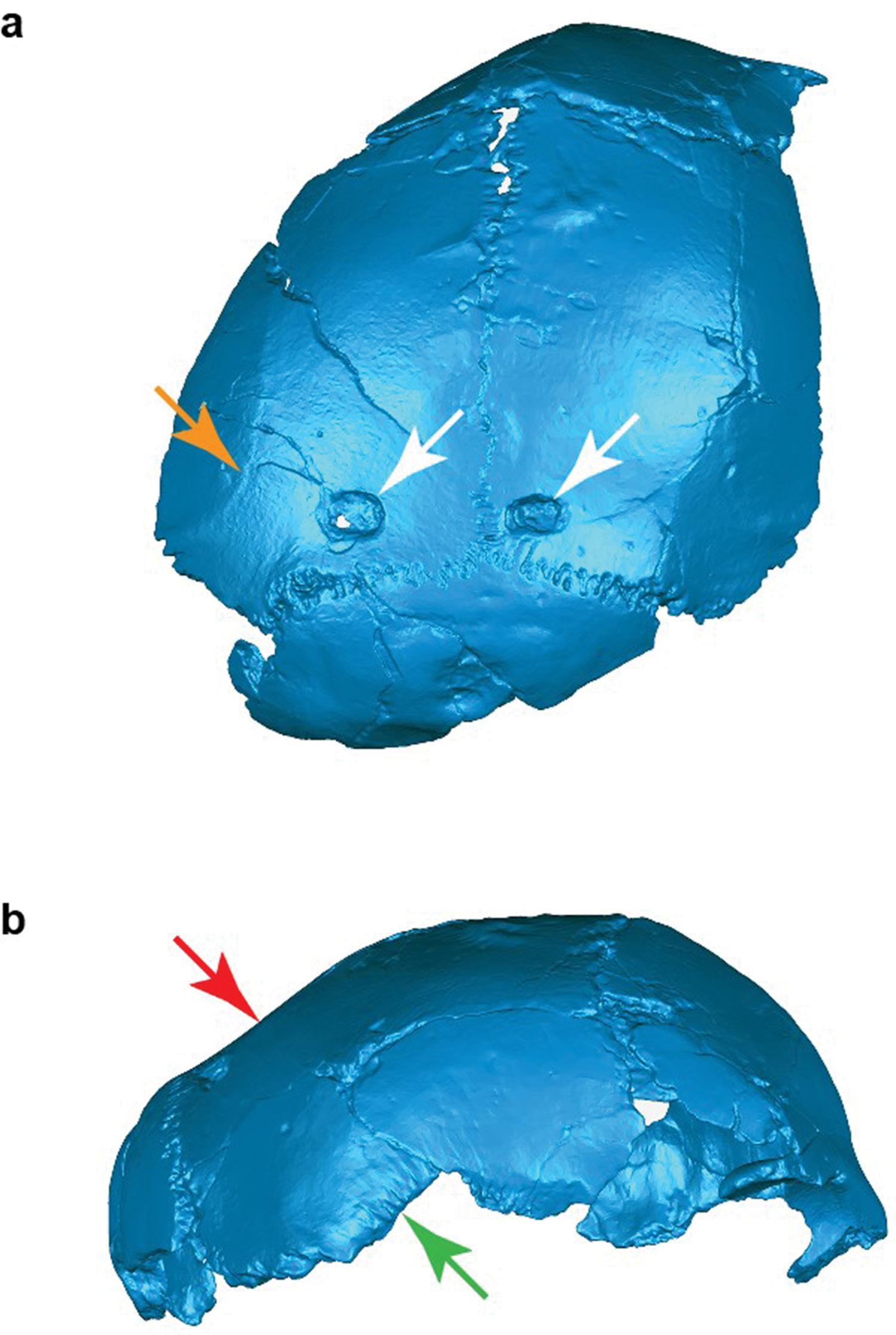
neurocranial vault is distorted on both the right and left sides, making a digital reconstruction highly subjective and of little diagnostic value. The individual evidently had a generally small brain, but estimates of its cranial capacity cannot be made with confidence.28 Nonetheless, aspects of preserved morphology challenge its traditional taxonomic attribution to Paranthropus and suggest affinities with Homo. The temporal lines are well separated and laterally positioned (Figure 1) – a configuration that is incompatible with adult P. robustus specimens that exhibit either a sagittal crest (in putative male specimens) or nearly convergent temporal lines (in female specimens).29 The KW 9000/9600 fossil from Kromdraai provides the only evidence for temporal line configuration in a subadult
P. robustus, and the superior temporal line is clearly closer to midline in the vicinity of bregma24 than the weakly expressed and more laterally positioned temporal lines exhibited by SK 54. Similarly, the juvenile P. aethiopicus specimen L338y-6 (whose sutures are as or more open than those of SK 54, implying a coarse similarity in age) exhibits welldeveloped, strongly convergent temporal lines30, further suggesting that SK 54 may not be Paranthropus. Kimbel et al.20 have previously argued that SK 54 preserves rugose striae parietalis that they suggest are correlated with a high degree of overlap between the temporal squama and parietal at the squamosal suture. They based their inference on the observation by Rak31 that juvenile H. sapiens from a Holocene population
Volume 120| Number 3/4 March/April 2024 116 https://doi.org/10.17159/sajs.2024/16387 Research Article We the hunted Page 2 of 5
Figure 1: Three-dimensional surface scans of SK 54 shown in (a) superoposterior and (b) lateral views. White arrows indicate puncture marks. Orange arrow indicates the left superior temporal line positioned laterally far from the sagittal suture. Red arrow indicates likely pre-lambdoidal flattening. Green arrow indicates the posterior aspect of the parietal portion of the squamosal suture that is straight and shows minimal overlap with the temporal bone.
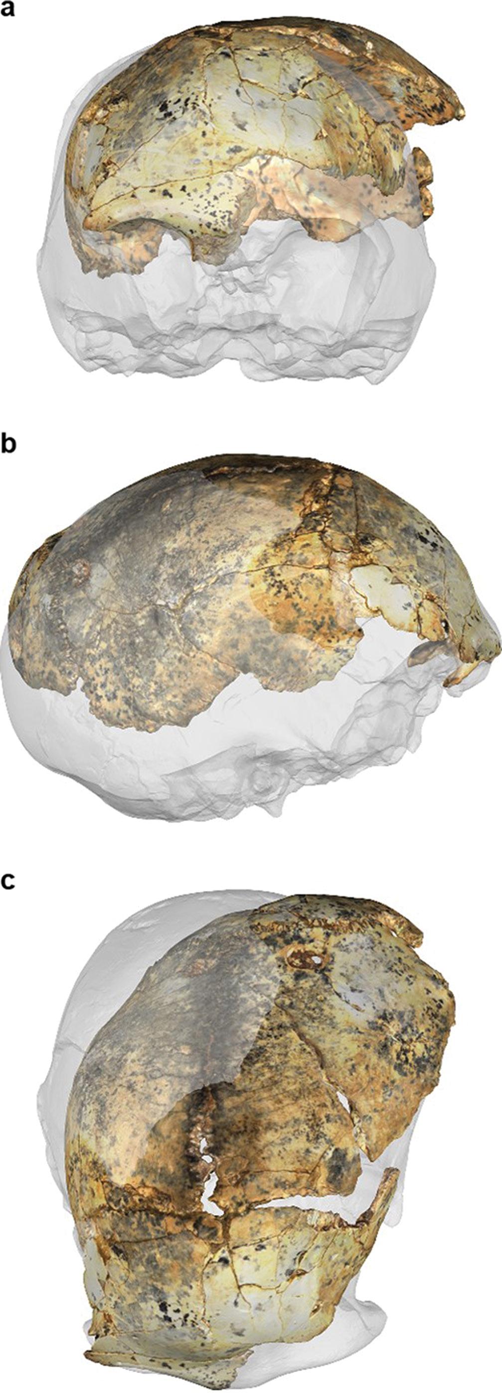
We the hunted Page 3 of 5
exhibited fine rather than rugose striae. However, the length of the striae parietalis preserved in SK 54 (Figure 1) are notably less than those of L338y-6 and adult P. robustus specimens DNH7, DNH152, and DNH155, and both the length and rugosity of SK 54’s striae closely resemble the condition in the juvenile H. erectus sensu lato specimen DNH 134. In our assessment, enough of the inferior bevelled edge of the right parietal (Figure 1) is preserved to indicate that the temporal and parietal portions of the squamosal suture would not have overlapped extensively, unlike the extensive overlap seen in both adult and juvenile Paranthropus. 30-32 Finally, contra Kimbel et al.20, the very wide separation of the superior temporal lines on the frontal bone argues against the inference that a frontal trigon would have developed in adulthood.
Two discrete traits of SK 54 may suggest affinities with Homo erectus sensu lato The preserved posterior portion of the squamosal suture is straight as it rises anteriorly and superiorly (Figure 1). Rightmire et al.33 note that, “A low temporal squama with a straight upper border passing downward toward asterion is a consistent marker for [H. erectus].” Moreover, SK 54’s parietal bones are flattened anterior to the lambdoidal suture (Figure 1), although there is distortion present in this region. Pre-lambdoidal flattening is a derived characteristic of many H. erectus specimens; in their description of the skulls from Dmanisi, Rightmire et al.33 state that:
There are also good indications that the Dmanisi skulls share at least a few (specialized?) characters with populations from the Far East. An example is provided by parasagittal flattening of the posterior vault. Flattening or even depression of the parietal surfaces is pronounced at Dmanisi, and it is common in the [H.] erectus crania from Sangiran in Java.
The fragmentary and deformed nature of SK 54 precludes a definitive taxonomic allocation but, heuristically, superimposing SK 54 onto H. erectus sensu lato specimen KNM-ER 4270034 demonstrates a striking similarity between the two specimens (Figure 2). We agree with Braga et al.24 that a provisional assignment of SK 54 to Homo seems warranted, and we argue that a tentative species-level allocation to H. erectus sensu lato is plausible. This assignment adds to the evidence for Homo at Swartkrans Member 1 Hanging Remnant that includes the juvenile cranium SK 27 that Clarke35 reclassified from P. robustus to Homo, and the suggested partial skull consisting of individual fossils SK 80, SK 846b, SK 84736 and sometimes also the mandible fragment SK 452 . At 1.9–1.8 Ma3, these fossils are slightly younger than the 2.04–1.95 Ma DNH 134 cranium from Drimolen Main Quarry that also shows affinities to Homo erectus32
Discussion
Brain’s work on cave taphonomy remains seminal, and his taphonomic assessment linking SK 54 with leopard predation is currently unchallenged. Assuming that those taphonomic conclusions remain valid, our taxonomic reassessment of SK 54 demonstrates that Homo was also prey for leopards in the early Pleistocene, and this characterisation could not be further removed from classic depictions of Homo the hunter and Paranthropus the hunted. Allocating SK 54 to Homo tempers the impetus for supposing that early Homo and P. robustus were differentially predated because of the former’s behavioural and technological advancement.
It is impossible to know with certainty how the history of palaeoanthropology might have been different had SK 54 been recognised as Homo when it was first discovered, but it is reasonable to infer that the impact of such a realisation would have been significant. Only 6 years prior to the publication of Brain’s1 now-classic paper, the description of the newly discovered H. habilis36 included an assessment of the relative tool-making skills and trophic positions of the new species and its contemporary, Zinjanthropus boisei (i.e. P. boisei):
While it is possible that Zinjanthropus and Homo habilis both made stone tools, it is probable that the latter was the more advanced tool maker and that the Zinjanthropus skull represents an intruder (or a victim) on a Homo habilis living site.37
Volume 120| Number 3/4 March/April 2024 117 https://doi.org/10.17159/sajs.2024/16387 Research Article
Figure 2: Superimposition of a three dimensional surface scan of SK 54 onto a cast of KNM-ER 42700 (transparent, scaled to 90% of its size) in (a) frontal, (b) right lateral, and (c) superior views. The specimens are aligned at their right orbital margins and circumorbital regions, which are the least distorted portions of SK 54.
Shortly thereafter, the highly influential Man the Hunter conference was held, followed by the publication of its accompanying edited volume38,39 that described hunting as a fundamentally important human adaptation. Brain’s2,3 interpretation of SK 54, based on an incorrect taxonomy, was therefore compatible with the thinking of the time, but it could have instead been a powerful challenge to conventional wisdom. Ideas, like species, evolve and have descendants, so the evidence presented here should prompt a reassessment of hypotheses concerning the biology, behaviour, and technological capabilities of Homo and Paranthropus that are derived from earlier ideas positing Homo as predator and Paranthropus as prey (for example, Lockwood et al.29). Our findings complement a recent zooarchaeological analysis showing that the appearance of H. erectus is not associated with increased evidence for hominin carnivory.38
Acknowledgements
We thank the DITSONG Natural History Museum and the hominin fossil curator Mirriam Tawane for facilitating access to the fossil hominin assemblage. We also thank the University of the Witwatersrand Evolutionary Studies Institute and the hominin fossil curators Bernhard Zipfel and Sifelani Jirah for facilitating access to the hominin fossil collection. We thank Kieran McNulty for sharing comparative data and contributing to discussions concerning hominin diversity at Drimolen. This research was funded and supported by HDR fee waivers and living scholarships from La Trobe University to J.M.M. and an Australian Research Council Discovery Grant DP170100056 to A.I.R.H. and D.S.S.
Competing interests
We have no competing interests to declare.
Authors’ contributions
J.M.M., A.B.L., A.I.R.H., S.E.B., and D.S.S. wrote the paper. J.M.M. and D.S.S. additionally participated in conceptualisation, data collection, sample analysis, and data analysis.
References
1. Brain CK. New finds at the Swartkrans australopithecine site. Nature. 1970;255:1112–1119. https://doi.org/10.1038/2251112a0
2. Brain CK. The hunters or the hunted? Chicago, IL: Chicago University Press; 1981.
3. Herries AIR. Chronology of the hominin sites of southern Africa. In: Oxford Research Encyclopedia of Anthropology. Oxford: Oxford University Press; 2022. https://doi.org/10.1093/acrefore/9780190854584.013.57
4. Brain CL. The probable role of leopards as predators of the Swartkrans australopithecines. S Afr Archaeol Soc. 1969;224:170–171. https://doi.org /10.2307/3888296
5. Hayward MW, Henschel P, O’Brien J, Hofmeyr M, Balme G, Kerley GIH. Prey preferences of the leopard (Panthera pardus). J Zool. 2006;270:298–313. https://doi.org/10.1111/j.1469-7998.2006.00139.x
6. White TD. The comparative biology of “robust” Australopithecus: Clues from context. In: Grine FE, editor. Evolutionary history of the “robust” australopithecines. Piscataway, NJ: Transaction Publishers; 1988. p. 449–484.
7. Pickering TR. Taphonomy of the Swartkrans hominid postcrania and its bearing onissuesofmeat-eatingandfiremanagement.In:StanfordCB,BunnHT,editors. Meat-eating and human evolution. New York: Oxford University Press; 2001. p. 33–51. https://doi.org/10.1093/oso/9780195131390.003.0003
8. Holloway RL. New australopithecine endocast, SK 1585, from Swartkrans, South Africa. Am J Phys Anthropol. 1972;37:173–186. https://doi.org/10.1 002/ajpa.1330370203
9. Blumenberg B, Todd NB. On the association between Homo and Australopithecus.CurrAnthropol.1974;15(4):386–388.https://doi.org/10.1086/201493
10. Susman RL. Pygmy chimpanzees and common chimpanzees: Models for the behavioral ecology of the earliest hominids. In: Kinzey WG, editor. Evolution of human behviour. Albany, NY: State University of New York Press; 1987. p. 72–86.
11. Lee-ThorpJ,ThackerayJF,VanderMerweN.Thehuntersandthehuntedrevisited. J Hum Evol. 2000;39:565–576. https://doi.org/10.1006/jhev.2000.0436
12. Pickering TR, Dominquez-Rodrigo M, Egeland CP, Brain CK. Beyond leopards: Tooth marks and the contribution of multiple carnivore taxa to the accumulation of the Swartkrans Member 3 fossil assemblage. J Hum Evol. 2004;46:595–604. https://doi.org/10.1016/j.jhevol.2004.03.002
13. Pickering TR. Underrated prey? Evol Anthropol. 2005;14:159–164. https://d oi.org/10.1002/evan.20070
14. Gommery D, Pickford M, Senut B. A case of carnivore-inflicted damage to a fossil femur from Swartkrans, comparable to that on a hominid femur representing Orrorin tugenensis, BAR 1003’00 (Kenya): Scientific notes. Ann Transvaal Mus. 2007;44:215–218. https://hdl.handle.net/10520/EJC83650
15. Pobiner BL. Paleoecological information in predator tooth marks. J Taphonomy. 2008;6:373–397.
16. Val A, Taru P, Steininger C. New taphonomic analysis of large-bodid primate assemblages from Cooper’s D, Bloubank Valley, South Africa. S Afr Archaeol Bull. 2014;69:49–58.
17. Arriaza MC, Aramendi J, Mate-Gonzalez MA, Yravedra J, Stratford D. The hunted or the scavenged? Australopith accumulation by brown hyenas at Sterkfontein (South Africa). Quat Sci Rev. 2021;273, Art. #107252. https://d oi.org/10.1016/j.quascirev.2021.107252
18. Wolpoff MH. Is the new composite cranium from swartkrans a small robust australopithecine? Nature. 1971;230:398–401. https://doi.org/10.1038/230 398a0
19. Wolpoff MH. Sagittal cresting in the South African australopithecines. Am J Phys Anthropol. 1974;40:397–408. https://doi.org/10.1002/ajpa.1330400312
20. Kimbel WH, White TD, Johanson DC. Cranial morphology of Australopithecus afarensis: A comparative study based on a composite reconstruction of the adult skull. Am J Phys Anthropol. 1984;64:337–388. https://doi.org/10.100 2/ajpa.1330640403
21. RakY, Kimbel WH, Moggi-Cecchi J, Lockwood CA, Menter C. The DNH 7 Skull of Australopithecus robustus from Drimolen (Main Quarry), South Africa. J Hum Evol. 2021;151:102913. https://doi.org/10.1016/j.jhevol.2020.102913
22. Tobias PV. Olduvai Gorge, Vol 2. The cranium and maxillary dentition of Australopithecus (Zinjanthropus) boisei. Cambridge: Cambridge University Press; 1967.
23. Clarke RJ. The cranium of the Swartkrans hominid SK 847 and its relevance to human origins. Johannesburg: University of the Witwatersrand; 1977.
24. Braga J, Wood BA, Zimmer VA, Moreno B, Miller C, Thackeray JF, et al. Hominin fossils from Kromdraai and Drimolen inform Paranthropus robustus craniofacial ontogeny. Sci Adv. 2023;9, eade7165. https://doi.org/10.1126/ sciadv.ade7165
25. Antón S. Natural history of Homo erectus. Am J Phys Anthropol. 2003; 122:126–170. https://doi.org/10.1002/ajpa.10399
26. Antón S. Developmental age and taxonomic affinity of the Mojokerto child, Java, Indonesia. Am J Phys Anthropol. 1997;102:497–514. https://doi.org /10.1002/(SICI)1096-8644(199704)102:4<497::AID-AJPA6>3.0.CO;2-P
27. Coqueugniot H, Hiblin J-J, Veillon F, Houet F, Jacob T. Early brain growth in Homo erectus and implications for cognitive ability. Nature. 2004;431:299–302. https://doi.org/10.1038/nature02852
28. Holloway RL, Broadfield DC, Yuan MS. The human fossil record: Brain endocasts – The paleoneurological evidence. Vol. 3. New York: Wiley-Liss; 2004. https://doi.org/10.1002/0471663573
29. Lockwood CA, Menter CG, Moggi-Cecchi J, Keyser AW. Extended male growth in a fossil hominin species. Science. 2007;318:1443–1446. https://d oi.org/10.1126/science.1149211
30. Rak Y, Howell CF. Cranium of a juvenile Australopithecus boisei from the Lower Omo Basin, Ethiopia. Am J Phys Anthropol. 1978;48:345–365. https: //doi.org/10.1002/ajpa.1330480311
31. RakY.Thefunctionalsignificanceofthesquamosalsuturein Australopithecus boisei. Am J Phys Anthropol. 1978;49:71–78. https://doi.org/10.1002/ajpa .1330490111
32. Herries AIR, Martin JM, Leece AB, Adams JW, Boschian G, Joannes-Boyau R, et al. Contemporaneity of Australopithecus, Paranthropus, and early Homo erectus in South Africa. Science. 2020;368:47. https://doi.org/10.1126/scie nce.aaw7293
Volume 120| Number 3/4 March/April 2024 118 https://doi.org/10.17159/sajs.2024/16387 Research Article
hunted Page 4 of 5
We the
33. Rightmire PG, Lordkipanidze D, Vekua A. Anatomical descriptions, comparative studies and evolutionary significance of the hominin skulls from Dmanisi, Republic of Georgia. J Hum Evol. 2006;50:115–141. https://doi.or g/10.1016/j.jhevol.2005.07.009
34. Spoor F, Leakey MG, Gathogo PN, Brown FH, Anton SC, McDougall I, et al. Implications of new early Homo fossils from Ileret, east of Lake Turkana, Kenya. Nature. 2007;448:688–691. https://doi.org/10.1038/nature05986
35. Clarke RJ. A juvenile cranium and some adult teeth of early Homo from Swartkrans, Transvaal. S Afr J Sci. 1977;73:46–49.
36. Clarke RJ, Howell FC, Brain CK. More evidence of an advanced hominid at Swartkrans.Nature.1970;225:1219–1222.https://doi.org/10.1038/2251219a0
We the hunted Page 5 of 5
37. Leakey LSB, Tobias PV, Napier JR. A new species of the genus Homo from Olduvai Gorge. Nature. 1964;202:7–9. https://doi.org/10.1038/202007a0
38. Lee RB, DeVore I, editors. Man the hunter. The first intensive survey of a single, crucial stage of human development – man’s once universal hunting way of life. Chicago, IL: Aldine; 1968.
39. Barr WA, Pobiner B, Rowan J, Faith JT. No sustained increased in zooarchaeological evidence for carnivory after the appearance of Homo erectus. Proc Natl Acad Sci USA. 2022;119, e2115540119. https://doi.org/ 10.1073/pnas.2115540119
Volume 120| Number 3/4 March/April 2024 119 https://doi.org/10.17159/sajs.2024/16387 Research Article
