Thermal Dispersion in a 2D rectangular block
Chaitanya Sai Kodali M.ScDepartment of Mechanical Engineering, Tennessee Technological University, Tennessee, Cookeville 38501
Abstract: The present work involves the numerical research a pore scale analysis is conducted to explore the actions of microscopic inertia and thermal dispersion in a porous medium. Thermal dispersion in porous media is an import phenomenon for Enhanced Oil Recovery methods including several other engineering applications in combustion and in steam injection systems. The results of thermal dispersion inside cross-flow tubular heat exchangers on heat transfer and temperature zone are numerically examined. Owing to the existence of barriers, thermal dispersion induced by fluid mixing plays a significant role in increasing heat transfer. Accurate calculations of the departure temperature and overall heat transfer rate must also be taken into consideration. The computational process analysis and simulation was developed using the ANSYS method. In this paper, a low Reynolds number flow is considered therefore, flow is regulated by Darcy's law. The present study demonstrates the shift in the centerline temperature values in specific flow directions with variations in relative thermal conductivity magnitude for thermal conductivity of the wood.
Keywords: Thermal conductivity, Thermal dispersion, Volume averaging, Tortuosity, Porosity, Reynolds number, Specific heat, grid generation, Representative elementary volume, porous media, gradient operation, liquid composite modeling.
1. INTRODUCTION
Our goal in this paper is to concentrate on the concept of thermal dispersion which occurs in the governing equation for non-isothermal flow through porous media. The concept of thermal dispersion increases the possibility of both the porous material's micro-structure and the influence of heat convection. The study of thermal dispersion in porous media typically takes advantage of the notion of representative elementary volume (REV), in which the transport equations are integrated [1–5]. The manufacturing processes of polymer composites such as liquid composite molding (LCM) are one of the most important applications of using thermal dispersion effect in the statistical simulation of the heat equation. Phelan et al.[3] demonstrated that, for single-scale porous material, the traditional volume averaging procedure can be used to extract the transport equation for thermochemical phenomena within the tows. Furthermore, Pedras and Lemos [4] were able to examine thermal dispersion in porous media using the conductivity values of both the solid and liquid phases. Yu determined and mapped out the thermal dispersion profiles of periodic porous structures [5].
In certain situations, an even more difficulty exists in the thermal governing equation owing to the existence of thermal dispersion [6] that occurs as a consequence of heat distribution at the pore size. This spreading is primarily attributed to the molecular heat diffusion, as well as the hydrodynamic mixing induced by the spontaneous fluid flow in a porous media. Greenkorn [7] listed nine mechanisms for the majority of pore-scale thermal spread. Yagi et al. [2] were the first to quantify the successful longitudinal thermal conductivity of the packed bed, taking full account of the thermal dispersion influence, and gradually finding that the longitudinal portion of the dispersion coefficient was much greater than its transverse part. This discovery, in spite of its importance, shocked them so much that they refused to report their findings for several years, according to Wakao and Kaguei [3]. Analytical procedure was recorded by Taylor [6] in a tube. Several theoretical and experimental efforts have since been made (e.g., Aris [7], Koch and Brady [8], Han et al. [9], and Vortmeyer [10]) to create useful associations to approximate thermal dispersion in porous media (see Kaviany [11]). In addition, Kuwahara et al. [12] and Nakayama et al. [13] performed a set of computational experiments by proposing a macroscopically uniform flow through a rod structure to expound the impact on thermal dispersion of microscopic velocity and temperature fields. It is also worth noting that Nakayama et al. [14] extracted from the volume-averaged version of Navier–Stokes and energy equations a thermal dispersion heat flux transmission equation and demonstrated
International Journal of Engineering Research and Reviews ISSN 2348-697X (Online)
Vol. 8, Issue 1, pp: (45-53), Month: January - March 2020, Available at: www.researchpublish.com
that it actually reduces to an algebraic formula for efficient thermal conductivity based on a gradient-type diffusion hypothesis. Careful study of temperature presence and full heat transfer capacity inside the tubular heat exchangers was conducted, and findings were seen
2. THEORETICAL MODELING
The fundamental principles of porous media theory are the methodology of local volume averaging and the usage of constant variables of field calculations, rather than instantaneous ones. Instead of modeling the microscopic resin flow through each filament, porous media theory predicts for the flow process average fields of velocity, pressure, and stress. This method is close to the average technique for homogeneous products used in continuum mechanics. This is more about measuring the position and velocity of each atom in a gas (i.e., the Lagrangian point of view), it uses the continuum theories to measure the velocity, pressure and temperature for specific areas comprising several atoms (i.e. the Eularian point of view). In order to extract the volume-averaged equations of energy, one must first consider the equations regulating energy conservation in the fluid and solid phases given below as Equations 1 and 2. ( ) (1) (2)
Note that ρ, c, and k represent density, specific heat capacity (in the case of the fluid it is the specific heat capacity at constant pressure, ), and thermal conductivity, respectively, where the subscripts f and s indicate quantities associated with either the fluid or solid phase. Also note that T represents temperature, u the fluid velocity vector, and t time.
Volume-averaging Equations 1 and 2 results in Equations 3 and 4 below. ( ) ( ∫ ̃ ) ∫ ̃ ̃ ̃
(3) ( ) ( ) ( ∫ ̃ ) ∫ ̃ (4)
Equations 3 and 4 are the un-simplified result of volume-averaging Equations 1 and 2, however, when considering highly conductive solid matrices, there are simplifications that can be made. With this simplification, the volume-averaged fluid energy equation becomes Equation 5 below. ( ) ∫ ̃ ̃ (5)
Note that the final term in Equation 5 represents thermal dispersion, while the second last term in Equation 5 and the last term in Equation 4 represent heat exchange between phases. In the solid energy equation, the tortuosity term is retained (as the second last term in Equation 4) since this term can be significant in forming the effective solid conductivity [21].
3. NUMERICAL SETUP
3.1 Computational Domain
The porous media computational domain under observation took the shape of a cylindrical pipe with a 0.229 m (9 in.) length and 0.0254 m (1in.) diameter. As will be listed in the assumptions and parameters section in Section 3.5 below, the chosen substance flow – engine oil – into the domain inlet is assumed to be uniform in the x-direction. Therefore, a
International Journal of Engineering Research and Reviews ISSN 2348-697X (Online)
Vol. 8, Issue 1, pp: (45-53), Month: January - March 2020, Available at: www.researchpublish.com
symmetric boundary condition was established onto the domain, allowing for the entire flow to be represented by one half of the cylindrical pipe width as shown in Figure 1. A preliminary analysis of flow effects in the pipe width (x-direction) showed that flow effects are primarily significant in two directions – throughout the pipe height and down the pipe stream. As a result, flow effects and stream changes could be accurately mapped in the two-dimensional mesh shown as Figure 2 The n-hexane (food coloring) droplet being injected into the pipe oil flow was directly modeled into the mesh, which showcases a 0.2 m (7.87 in.) by 0.1 m (3.94 in.) cross-section, and the mesh was refined to emphasize flow effects and changes around the injection. The n-hexane droplet was labeled as an injection in order to allow for access to relevant injection property implementations and calculations in the ANSYS solution setup. The flow cross section side edge nearest to the injection – on its left – was labeled as the flow inlet while the remaining side edge on the injection’s right was labeled as the flow outlet. The cross-section top and bottom edges were labeled as the flow profile walls.
3.2 Model Setup
The aforementioned cylindrical symmetric computational domain and representative rectangular two-dimensional crosssection were set up in ANSYS Workbench using the Fluent analysis system and the Design Modeler Geometry builder function. All size dimensions – the 0.0254 m (1 in.) by 0.229 m (9in.) pipe and the 0.2 m (7.87 in.) by 0.1 m (3.94 in.) cross-section – were defined as fixed and originated in the XY plane origin to allow for minimum domain displacement considerations in property value calculations such as temperature and velocity. The two-dimensional model including the injected particle representation was made as a plane surface from a sketch in order to allow for calculations and property plotting throughout the entire profile.
Once the two-dimensional rectangular cross-section geometry was established, the cross-section mesh was defined. The primary meshing objective was to minimize the number of calculation grid nodes – particularly those with complex geometries or non-parallel and non-perpendicular orientations to either the domain walls and/or the injected particle –without compromising the integrity or accuracy of the necessary property calculations. This was done using the second refinement mesh option available in the ANSYS Fluent mesh creator, thereby producing the mesh shown in Figure 2 above. The resulting mesh contained approximately 5200 nodes representing approximately 5000 elements with an average element quality of 0.876 out of a maximum quality value of 1. This was far lower number than the one million nodes that would be needed to represent the entire cylindrical pipe computational domain shown in Figure 1 with a similar element quality. This results in the 2-D cross section calculations being much faster and requiring much less time for completion than those of the cylindrical pipe domain, thereby making the 2-D cross section an ideal choice to represent the flow domain.
The entire two-dimensional cross-section was set as porous media with a defined porosity in order to activate Darcy’s Law and its effects on flow temperature and velocity. In addition, the energy equation was activated in order to allow for a set initial temperature and flow temperature mapping with respect to time in the rectangular cross-section. Finally, a laminar viscous flow model was selected for the engine oil. This allows for the oil flow velocity to be properly represented with the low flow speed needed to achieve a Reynolds Number less than 10. This low oil velocity along with the remaining boundary and initial conditions needed to properly represent the n-hexane drop injection tests are shown in the following boundary and initial conditions section.
3.3 Boundary and Initial Conditions
In order to properly model the n-hexane particle injection flow within the engine oil flowing through the test cylindrical pipe, several initial conditions regarding both the n-hexane particle and engine oil velocities were considered along with several heat-related boundary conditions along the cylindrical pipe. The initial velocity of the flowing engine oil was determined with the Reynolds number equation shown as Equation 6 below:
(6)
In this Reynolds number equation, represents the engine oil density of 889 kg/m3 (55.50 lbm/ft3) V represents the initial engine oil flow velocity, L represents the characteristic length of the flow path – in this case represented by the cylinder pipe diameter of 0.0254 m (1 in.) – and represents the engine oil dynamic or absolute viscosity of 1.06 kg/m-s (0.712 lbm/ft-s). For the current experiment, a creeping flow with a Reynolds number of approximately 0.025 was desired, so an initial engine oil flow velocity of 0.00126 m/s (0.248 ft/min) was calculated to be the desired flow speed. This speed was
International Journal of Engineering Research and Reviews ISSN 2348-697X (Online)
Vol. 8, Issue 1, pp: (45-53), Month: January - March 2020, Available at: www.researchpublish.com
set at the cross-section inlet. For the flow outlet, the external flow gauge pressure was set to zero due to flow environment assumptions that will be elaborated on the assumptions and parameter section.
The flow two-dimensional cross-section was set as insulated in the radial y-direction since any temperature differences on the engine oil flow region may alter the oil’s viscosity to an extent that would significantly affect the oil flow Reynolds number during flow. As mentioned before, all property effects and changes in the selected domain are negligible in the radial x-direction, thereby allowing the domain to be represented as two-dimensional and setting a boundary condition allowing for the removal of all x-direction calculation terms, significantly reducing overall calculation steps and time. Finally, the porosity of the engine oil flow region (i.e. either the cylindrical pipe or the two-dimensional cross section representation) was predetermined to be 0.2. This was set as a defined condition in ANSYS Fluent that was directly implemented into the Darcy’s Law equations used to characterize our porous media flow. The results from the current simulation were compared to those obtained by an experimental setup with identical dimensions and conditions designed by William Alston and Kade Howard.
3.4 Grid Generation
In order to determine the proper grid density for this experiment, a grid independence study was conducted using the flow force values on the wall surface body. These flow force values were plotted against the pipe length for several grid densities as shown in Figure 3. As can be seen in Figure 3, a grid density of 5550 nodes is sufficient to ensure that simulation results such as wall static pressure will be close to accurate value. Therefore, the cylindrical pipe mesh was fitted to contain 5200 nodes.
3.5 Assumptions and Parameters
In order to simulate the engine oil flow within the rectangular cross section of the 0.229 m (9 in.). long cylindrical pipe in a manageable computational time frame, all simplifying assumptions on pipe, flow substance, and flow path characteristics that were found to not significantly influence the injection flow path were made. The main assumption of flow effects on properties and calculation values being negligible in the radial x-direction allowed for the flow model to be simplified into a two-dimensional rectangular cross-section representation in the first place. Another assumption was that the pipe, engine oil, and injected n-hexane droplet all maintain constant chemical composition and physical properties – i.e. density and viscosity – throughout the flow duration since no significant external temperature, pressure, or chemical changes were imposed throughout the flow. In addition, the environment surrounding the flow pipe was assumed to provide no external pressure source outside of air. Therefore, the flow outlet gauge pressure could be set to zero. Finally, the injected droplet was assumed to be insolvent and inert, meaning that it did not dissolve into the engine oil flowing through the pipe and did not have an initial velocity before flowing with the engine oil. This assumption was validated by the insolvency of n-hexane into engine oil along with the slow speed at which the particle was injected into the cylindrical pipe by Alston and Howard in their experimental setup.
4. RESULTS AND DISCUSSION
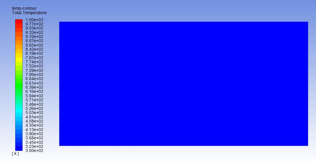
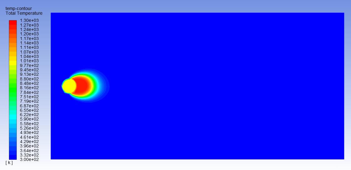
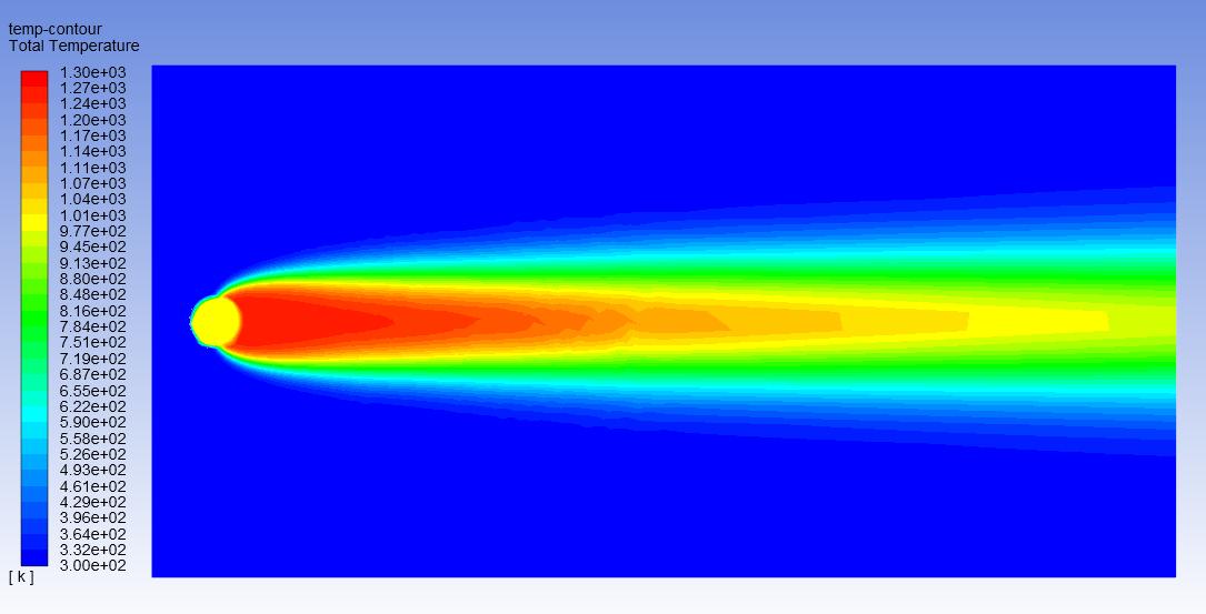
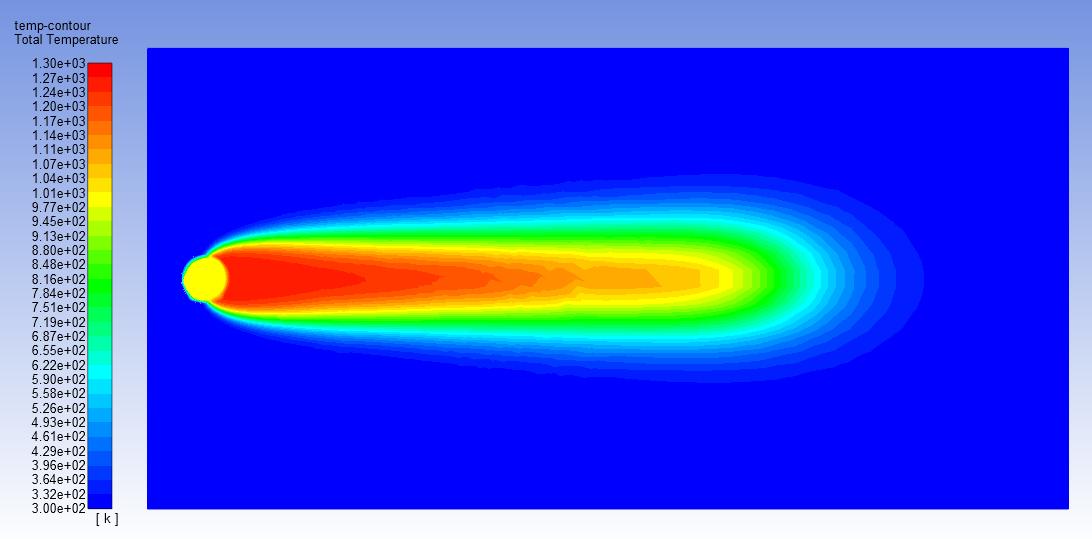
Once the numerical model was fully established with the configurations and assumptions detailed in the numerical analysis section above, the corresponding flow was activated using ANSYS Fluent. A time representation of 25 seconds was required for each test since this was the amount of time elapsed necessary for the injected droplet flow to reach a steady state. A dynamic temperature contour map of the mesh was developed to showcase flow progress across the modeled pipe section. In addition, the wooden pipe was labeled anisotropic, allowing flow relative viscosity and temperature to be defined and changed directly. The flow temperature profiles at four particular time steps – pre-flow profile, flow after five second elapsed time, flow after ten seconds elapsed time, and flow profile at steady state after 25 seconds – were modeled for the anisotropic injection flow with XX component equal to 1 and YY component equal to 5 and with n-hexane injection particle temperature at 1000 K (726.85oC) surrounded by engine oil at 300 K (26.85oC) These flow profiles are shown in Figures 1-4.
From Figures 1-4, a complete picture of the injected particle flow progression is seen. At the initial state – time t=0 as shown in Figure 1 – the n-hexane particle has not been injected yet so the entire flow profile consists only of the engine oil at 300 K (26.85oC). After the first second – time t=1 as shown in Figure 2 – the n-hexane particle has been injected and it begins to travel down the engine oil flow stream, dispersing enough heat to make the flow path part immediately next to the particle reach a higher temperature than the initial 1000 K (726.85oC) injection temperature while dispersing additional heat in some of the positive and negative y-directions. After the particle flows for ten seconds – time t=10 as
International Journal of Engineering Research and Reviews ISSN 2348-697X (Online)
Vol. 8, Issue 1, pp: (45-53), Month: January - March 2020, Available at: www.researchpublish.com
shown in Figure 3 – an overall picture of the final flow profile begins to emerge where the particle heat is dispersed in a diminishing conical path. This means that, as the particle flows downstream its heat energy dissipates, reducing in power and total heat transfer, and thus total temperature change in the downstream z-direction while increasing the total area where temperature change does occur, albeit at a lower magnitude, in the stream y-direction. Once the injected particle flow completes its path – time t=25 as shown in Figure 4 – the final flow temperature profile shows that the injected particle does make it across the entire cross-section in the downstream z-direction, spreading out its heat transfer energy onto a greater portion of the pipe height (y-direction) as it progresses while simultaneously gradually losing the amount of heat transfer energy directly downstream in the z-direction in a manner reminiscent of the heated, flaming debris at the tail of an asteroid burning up in Earth’s atmosphere without being completely destroyed before it hits land.
One key observation from the flow path is that the line across the center of the injected particle, in this case being the center of the pipe since the particle was injected at the pipe center, shows the greatest amount of heat transfer and thus the greatest temperature change. As a result, an observation of the relative heat dissipated in any path of this injected particle flow can be represented by a plot of the centerline temperature at the end of the total flow. This allows for a convenient and clear observation of the heat dissipation differences between flows with different wood pipe thermal conductivity anisotropic configurations and relative magnitudes. As a result, these flow differences were plotted with variation of the anisotropic thermal conductivity XX and YY flow components shown in Figure 5 and variation of the thermal conductivity relative magnitude shown in Figure 6.
As can be seen in Figure 5, changing the XX component relative to the YY component of the flow anisotropic wood thermal conductivity has no significant effect on flow centerline temperature while increasing the YY component relative to the XX component results in a centerline temperature diminishing at a greater rate past the initial particle geometry. This shows that the finite amount of heat transfer emanated from the flowing injection particle is spread in a function along the y-direction and not along the z-direction represented by the XX component. For all flows with YY components equivalent to 1, this heat transfer leads to a centerline temperature of around 1175 K (901.85oC) at the end of the 0.2 m (7.87 in.) flow cross section. For the flow with YY component five times that of the XX component, this end centerline temperature reduces to approximately 975 K (701.85oC) while the flow with YY component ten times that of the XX component has its end centerline temperature reduced to approximately 825 K (551.85oC)
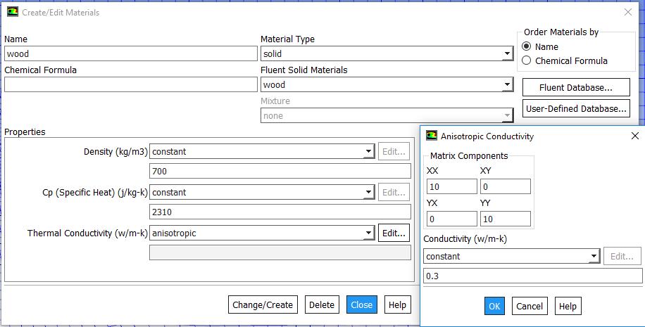
From Figure 6, it can be seen that increasing the relative magnitude of the anisotropic wood thermal conductivity has a similar effect to increasing the YY flow component relative to the XX flow component. This implies that the heat transfer is inversely related to the thermal conductivity of its vessel pipe and that the total function representing heat dissipation of the injected particle includes both the relative thermal conductivity magnitude and the magnitude of the YY anisotropic flow component with respect to the XX flow component. At the default relative magnitude of 1, the end centerline temperature is at around 1175 K (901.85oC). For relative magnitudes of 5, 10, and 20, the end centerline temperature is approximately 975 K (701.85oC), 825 K (551.85oC), and 700 K (426.85oC) respectively. A representation of anisotropic matrix components is depicted in figure 7 It can be seen that the centerline temperature paths from the relative anisotropic wood thermal conductivity magnitudes of one, five, and ten almost perfectly correspond to the centerline temperature paths where the YY anisotropic wood thermal conductivity component is respectively equal to, five times that of, and ten times that of the XX component. This bolsters the assumption that all changes in the relative thermal conductivity magnitude for the wood thermal conductivity is in the flow YY direction.
5. CONCLUSION
In this paper, the non-isothermal flow through porous media is studied numerically. The quantification of the thermal dispersion effect that enhances heat transfer in porous-media flows has been attempted. The three-dimensional porous reactor model could be represented with a two-Dimensional cross-sectional area due to insignificant thermal changes in pipe X-direction. The injected particle droplet moves quickly along cylindrical wooden pipe and it significantly increases temperature of engine oil which is in contact with the droplet. The magnitude of unidirectional anisotropic thermal conductivity components XX and YY are directly related to the maximum temperature that reached inside the pipe. One thing we can find from Figure 5 and 6 is, the function that describes heat dissipation from injection particles is function of both relative magnitude of its vessel anisotropic thermal conductivity and relative magnitude of YY flow component to the XX flow component. Our next potential study will involve us determining the way to directly calculate the anisotropic thermal conductivity for a specific fluid.
International Journal of Engineering Research and Reviews ISSN 2348-697X (Online) Vol. 8, Issue 1, pp: (45-53), Month: January - March 2020, Available at: www.researchpublish.com
NOMENCLATURE
ρ = Density of fluid (kg/m3)
C = Specific heat (J/kg-K)
k = Thermal Conductivity (W/m-K)
T = Temperature (K)
u = Fluid velocity vector (m/s)
t = Time (s)
XY = Plane in respective co-ordinate direction
XX, YY = Components in respective co-ordinate direction
Re = Reynolds number
L = Length of flow path (m)
μ = Oil dynamic viscosity (Kg/m-s)
V = Initial engine oil flow velocity (m/s)
ε = Porosity
A = Area of flow path (m2)
dA = Change in area = gradient operation
< > = Volume averaged concentration
˜ = deviation of concentration
Subscripts
f = Fluid phase
s = Solid phase
p = specific heat at constant pressure
REFERENCES
[1] C.T. Hsu, P. Cheng, Thermal dispersion in a porous medium, Int. J. Heat Mass Transfer 33 (1990) 1587–1597.
[2] M. Kaviany, Principles of Heat Transfer in Porous Media, second ed., Springer, New York, 1995.
[3] J.A. Ochoa-Tapia, S. Whitaker, Heat transfer at the boundary between a porous medium and a homogeneous fluid, Int. J. Heat Mass Transfer 40 (11) (1997) 2691–2707.
[4] Pedras, M. and Lemos, M. Thermal dispersion in porous media as a function of the solid–fluid conductivity ratio.
[5] Yu, B. ASME Journal Discussion: ‘‘A Numerical Study of Thermal Dispersion in Porous Media’’ and ‘‘Numerical Determination of Thermal Dispersion Coefficients Using a Periodic Porous Structure’’.
[6] C. Moyne, Two-equation model for a diffusive process in porous media using the volume averaging method with an unsteady-state closure, Adv. Water Resour. 20 (2–3) (1997) 63–76.
[7] Phelan, F.R., Modeling of Microscale Flow in Fibrous Porous Media, Springer-Verlag, New York Inc., USA, 1991.
[8] Nield, D.A., Bejan, A., Convection in Porous Media, Springer, USA, 2006
[9] Robert A. Greenkorn, Flow Phenomena in Porous Media, New York and Besel, USA, 1983.
[10] Yagi S, Kunii D, Wakao N (1960) Studies on axial effective thermal conductivities in packed beds. AIChE Journal. 6:543–546
[11] Wakao N (1996) Kaguei S. Heat and mass transfer in packed beds. Gordon and Breach, New York
[12] Taylor GI (1953) Dispersion of solute matter in solvent flowing slowly through a tube. Proc. Roy. Soc. London 15:1787–1806
International Journal of Engineering Research and Reviews ISSN 2348-697X (Online) Vol. 8, Issue 1, pp: (45-53), Month: January - March 2020, Available at: www.researchpublish.com
[13] Aris R (1956) On the dispersion of a solute in a fluid flowing through a tube. Proc R Soc Lond 235:67–77
[14] Koch DL, Brady JF (1985) Dispersion in fixed beds. J Fluid Mech 154:399–427
[15] Han NW, Bhakta J, Carbonell RG (1985) Longitudinal and lateral dispersion in packed beds: Effect of column length and particle size distribution. AIChE J 31:277–288
[16] Vortmeyer D (1975) Axial heat dispersion in packed beds. Chem Eng Sci 30:999–1001
[17] Kaviany M (1991) Principles of heat transfer in porous media. Springer, New York, pp 115–151
[18] Kuwahara F, Nakayama A, Koyama H (1996) A numerical study of thermal dispersion in porous media. Trans ASME J Heat Trans 118:756–761
[19] Nakayama A, Kuwahara F, Umemoto T, Hayashi T (2002) Heat and fluid flow within an anisotropic porous medium. Trans ASME J Heat Trans 124:746–753
[20] Nakayama A, Kuwahara F, Kodama Y (2006) An equation for thermal dispersion flux transport and its mathematical modelling for heat and fluid flow in a porous medium. J Fluid Mech 563:81–96
[21] S. Krishnan, J.Y. Murthy, S.V. Garimella, J. Heat Transfer 128, 793 (2006)
APPENDICES - A
Figure 1: Initial Temperature Profile of Anisotropic Flow with XX=1 and YY=1
Figure 2: Temperature Profile of Anisotropic Flow with XX=1 and YY=1 after 1 Second Elapsed Flow Time
Research Publish Journals
Anisotropic XX=1 YY=1
Anisotropic XX=1 YY=5
Anisotropic XX=1 YY=10
Anisotropic XX=5 YY=1 Anisotropic XX=10 YY=1
International Journal of Engineering Research and Reviews ISSN 2348-697X (Online) Vol. 8, Issue 1, pp: (45-53), Month: January - March 2020, Available at: www.researchpublish.com
Centerline Temperature at Various Anisentropic Wood Thermal Conductivity Magnitude Configurations
Centerline Temperature (K)
1200
1000
800
600
400
200
0
Relative Magnitude 1
Relative Magnitude 5
Relative Magnitude 10
Relative Magnitude 20
1400 0 0.02 0.04 0.06 0.08 0.1 0.12 0.14 0.16 0.18 0.2
Centerline Position (m)
Figure 6: Centerline Temperatures for Various Anisotropic Thermal Conductivity Relative Magnitude Configurations
Figure 7: Representation of anisotropic matrix components
