Principles of Corporate Finance 12th Edition Brealey Solutions Manual

CHAPTER 2

How to Calculate Present Values

The values shown in the solutions may be rounded for display purposes. However, the answers were derived using a spreadsheet without any intermediate rounding.

Answers to Problem Sets

1. Ct = PV × (1 + r)t C8 = $100 × 1.158 C8 = $305.90

Est time: 01-05

2. PV = Ct / DFt DFt = $125 / $139 DFt = .8993

Est time: 01-05

3. PV = Ct / (1 + r)t PV = $374 / 1.099 PV = $172.20

Est time: 01-05

4.

b. NPV = PV – investment NPV = $1,003.28 – 1,200 NPV = –$196.72

Est time: 01-05

5. a. False. The opportunity cost of capital varies with the risks associated with each individual project or investment. The cost of borrowing is unrelated to these risks.

b. True. The opportunity cost of capital depends on the risks associated with each project and its cash flows.

c. True. The opportunity cost of capital is dependent on the rates of returns shareholders can earn on the own by investing in projects with similar risks

d. False. Bank accounts, within FDIC limits, are considered to be risk-free. Unless an investment is also risk-free, its opportunity cost of capital must be adjusted upward to account for the associated risks.

Est time: 01-05

6. NPV = C / r – investment

Copyright © 2017 McGraw-Hill Education. All rights reserved. No reproduction or distribution without the prior written consent of McGraw-Hill Education.

NPV = $138 / 09 $1,548

NPV = $14 67

Est time: 01-05

7. PV = C / (r – g)

PV = $4 / ( 14 04)

PV = $40

Est time: 01-05

8.

a. PV = C / r

PV = $1 / .10

PV = $10

b. PV7 = (C8 / r)

PV0 approx = (C8 / r) / 2

PV0 approx = ($1 / .10) / 2

PV0 approx = $5

c. A perpetuity paying $1 starting now would be worth $10 (part a), whereas a perpetuity starting in year 8 would be worth roughly $5 (part b). Thus, a payment of $1 for the next seven years would also be worth approximately $5 (= $10 – 5).

d. PV = C / ( r g)

PV = $10,000 / (.10 .05)

PV = $200,000

Est time: 06-10

9. The basic present value formula is: PV = C / (1 + r)t

a. PV = $100 / 1.0110

PV = $90.53

b. PV = $100 / 1.1310

PV = $29.46

c. PV = $100 / 1.2515 PV = $3.52

d.

Est time: 01-05

10. a. FV = C × ert

FV = $1,000 × e.12 x 5

FV = $1,822.12

b. PV = C / ert

Copyright © 2017 McGraw-Hill Education. All rights reserved. No reproduction or distribution without the prior written consent of McGraw-Hill Education.

PV = $5,000,000 / e.12 × 8

PV = $1,914,464

c. PV = C (1 / r – 1 / rert)

PV = $2,000 (1 / .12 – 1 / .12e .12 x 15)

PV = $13,911.69

Est time: 01-05

11.

a. Ct = PV × (1 + r)t

Ct = $10,000,000 x (1.06)4

Ct = $12,624,770

b. Ct = PV × [1+ (r / m)mt

Ct = $10,000,000 × [1 + (.06 / 12)]12 × 4

Ct = $12,704,892

b. Ct = PV × ert

Ct = $10,000,000 × e.06 × 4

Ct = $12,712,492

Est time: 01-05

12.

a. PV = Ct / (1 + r)t

PV = $10,000 / 1.055

PV = $7,835.26

b. PV = C((1 / r) – {1 / [r(1 + r)t]})

PV = $12,000((1 / .08) – {1 / [.08(1.08)6]})

PV = $55,474.56

c. Ct = PV × (1 + r)t

Ct = ($60,476 55,474.56) × 1.086

Ct = $7,936.66

Est time: 06-10

13.

a. DF1 = 1 / (1 + r)

r = (1 – .905)/ .905

r = .1050, or 10.50%

b. DF2 = 1 / (1 + r)2

DF2 = 1 / 1.1052

DF2 = .8190

c. PVAF2 = DF1 + DF2

PVAF2 = .905 + .819

PVAF2 = 1.7240

d. PVA = C × PVAF3

PVAF3 =$24.65 / $10

PVAF3 = 2.4650

Copyright © 2017 McGraw-Hill Education. All rights reserved. No reproduction or distribution without the prior written consent of McGraw-Hill Education.

e. PVAF3 = PVAF2 + DF3

DF3 = 2.465 – 1.7240

DF3 = .7410

14.

= $86,739.66

b. After five years, the factory’s value will be the present value of the five remaining year’s of cash flows.

16. The opportunity cost of capital refers to the rate of return a firm’s shareholders could earn on their own by investing at the same level of risk. Thus, when a firm considers a new project, it is the risk level of the project that determines opportunity cost of capital for that project.

Copyright © 2017 McGraw-Hill Education. All rights reserved. No reproduction or distribution without the prior written consent of McGraw-Hill Education.

$ 62,258.56

Est time: 01-05

18. a. NPV = –Investment + PVAoperating cash flows – PVrefits + PVscrap value

NPV = –$8,000,000 + ($5,000,000 – 4,000,000) × ((1 / .08) – {1 / [.08(1.08)15]}) –($2,000,000 / 1.085 + $2,000,000 / 1.0810) + $1,500,000 / 1.0815

NPV = –$8,000,000 + 8,559,479 – 2,287,553 + 472,863

NPV = –$1,255,212

b. The cost of borrowing does not affect the NPV because the opportunity cost of capital depends on the use of the funds, not the source.

Est time: 06-10

19. a. PV = C0

PV = $100,000

b. PV = Ct / (1 + r)t PV = $180,000 / 1.125

PV = $102,136.83

c. PV = C / r

PV = $11,400 / .12

PV = $95,000

d. PV = C × ((1 / r) – {1 / – [r(1 + r)t]})

PV = $19,000 × ((1 / .12) – {1 / – [.12(1.12)10]})

PV = $107,354.24

e. PV = C / (r – g)

PV = $6,500 / (.12 .05)

PV = $92,857.14

Prize (d) is the most valuable because it has the highest present value.

Est time: 01-05

20. C = PVA / ((1 / r) – {1 / [r(1 + r)t]})

C = $20,000 / ((1 / .08) – {1 / [.08(1 + .08)12]})

C = $2,653.90

Est time: 01-05

Copyright © 2017 McGraw-Hill Education. All rights reserved. No reproduction or distribution without the prior written consent of McGraw-Hill Education.

21. PV = Ct / (1 + r)t

PV = $20,000 / 1.105

PV = $12,418.43

C = PVA / ((1 / r) – {1 / [r(1 + r)t]})

C = $12,418.43 / ((1 / .10) – {1 / [.10 (1 + .10)5]})

C = $3,275.95

Est time: 06-10

22. The fact that Kangaroo Autos is offering “free credit” tells us what the cash payments are; it does not change the fact that money has time value.

Present value of payments to Kangaroo Auto:

PV = Down payment + C × ((1 / r) – {1 / [r(1 + r)t]})

PV = $1,000 + $300 × ((1 + .0083) – {1 / [.0083(1 + .0083)30]})

PV= $8,938.02

Present value of car at Turtle Motors:

PV = price of car – discount

PV = $10,000 – 1,000

PV = $9,000

Kangaroo Autos offers the best deal because it has the lower present value of costs.

Est time: 01-05

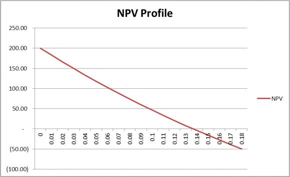
23. Use the formula: NPV =

The figure below shows that the project has a zero NPV at about 13.65%.

Copyright © 2017 McGraw-Hill Education. All rights reserved. No reproduction or distribution without the prior written consent of McGraw-Hill Education.

NPV13.65% = –$36.83

c Est time: 06-10

24.

a. PVOA = C / r

PVOA = $100 / .07

PVOA = $1,428.57

b. PVAD = C / r × (1 + r)

PVAD = $100 / .07 × (1 + .07)

PVAD = $1,528.57

c. To find the present value with payments spread evenly over the year, use the continuously compounded rate that equates to 7% compounded annually. This rate is found using natural logarithms.

PVCC = C / rCC

PVCC = $100 / Ln(1 + .07)

PVCC = $1,478.01

For informational purposes, the continuously compounded rate is:

Ln(1 + .07) = .0677, or 6.77%

The sooner payments are received, the more valuable they are.

Est time: 06-10

Copyright © 2017 McGraw-Hill Education. All rights reserved. No reproduction or distribution without the prior written consent of McGraw-Hill Education.

25.

a. PV = C / r PV = $1 billion / .08

PV = $12.5 billion

b. PV = C / (r – g)

PV = $1 billion / (.08 – .04)

PV = $25.0 billion

c. PV = C × ((1 / r) – {1 / [r (1 + r)t]})

PV = $1 billion × ((1 / .08) – {1 / [.08(1 + .08)20]})

PV = $9.818 billion

d. The continuously compounded equivalent to an annually compounded rate of 8% is approximately 7.7%, which is computed as:

Ln(1.08) = .077, or 7.7%

PV = C × {(1 / r) – [1 / (r × ert)]}

PV = $1 billion × {(1 / .077) – [1 / (.077 – e.077 × 20)]}

PV = $10.206 billion

This result is greater than the answer in Part (c) because the endowment is now earning interest during the entire year.

Est time: 06-10

26. Annual compounding:

Ct = PV × (1 + r)t

C20 = $100 × 1.1520

C20 = $1,636.65

Continuous compounding:

Ct = PV × ert

C20 = $100 × e.15 × 20

C20 = $2,008.55

Est time: 01-05

27. One way to approach this problem is to solve for the present value of:

Copyright © 2017 McGraw-Hill Education. All rights reserved. No reproduction or distribution without the prior written consent of McGraw-Hill Education.

(1) $100 per year for 10 years, and

(2) $100 per year in perpetuity, with the first cash flow at year 11.

If this is a fair deal, these present values must be equal, and thus we can solve for the interest rate (r).

The present value of $100 per year for 10 years is:

PV = C × ((1 / r) – {1 / [r(1 + r)t]})

PV = $100 × ((1 / r) – {1 / [r(1 + r)10]})

The present value, as of year 0, of $100 per year forever, with the first payment in year 11, is:

PV = (C / r) / (1 + r)t

PV = ($100 / r) / (1 + r)10

Equating these two present values, we have:

Using trial and error or algebraic solution, we find that r = 7.18%.

Est time: 06-10

b.

C

C

C

C

c.

C

C

Copyright © 2017 McGraw-Hill Education. All rights reserved. No reproduction or distribution without the prior written consent of McGraw-Hill Education.

The preferred investment is (c) because it compounds interest faster and produces the highest future value at any point in time.

Est time: 06-10

29. First, find the semiannual rate that is equivalent to the annual rate:

1 + r = (1 + r / 2)2

1.08 = (1 + r / 2)2

r / 2 = 1.08.5 – 1

r = .039230, or 3.9230%

PV = C 0 + C × ((1 / r) – {1 / [r(1 + r)t]})

PV = $100,000 + $100,000 × ((1 / .039230) – {1 / [.039230(1 + .039230)9]})

PV = $846,147.28

Est time: 06-10

30.

a. PV = C × ((1 / r) – {1 / [r(1 + r)t]})

PV = ($9,420,713 / 19) × ((1 / .08) – {1 / [.08(1 + .08)19]})

PV = $4,761,724

b. PV = C × ((1 / r) – {1 / [r(1 + r)t]})

$4,200,000 = ($9,420,713 /

Using Excel or a financial calculator, we find that r = 9.81%.

Copyright © 2017 McGraw-Hill Education. All rights reserved. No reproduction or distribution without the prior written consent of McGraw-Hill Education.

Est time: 06-10

32. a. PV = C × ((1 / r) – {1 / [r(1 + r)t]})

C = $2,000,000 / ((1 / .08) – {1 / [.08(1 + .08)15]})

C = $233,659.09

b. r = (1 + R) / (1 + h) – 1

r = 1.08 / 1.04 – 1

r = .0385, or 3.85%

PV = C × ((1 / r) – {1 / [r(1 + r)t]})

C = $2,000,000 / ((1 / .0385) – {1 / [.0385(1 +.0385)15]})

C = $177,952.49

The retirement expenditure amount will increase by 4% annually.

Est time: 06-10

33. a. PV = C × ((1 / r) – {1 / [r(1 + r)t]})

PV = $50,000 × ((1 / .055) – {1 / [.055(1 + .055)12]})

PV = $430,925.89

b. Since the payments now arrive six months earlier than previously:

PV = $430,925.89 × {1 + [(1 + .055).5 – 1]}

PV = $442,617.74

Est time: 06-10

34. Ct = PV × (1 + r)t

Ct = $1,000,000 × (1.035)3

Ct = $1,108,718

Annual retirement shortfall = 12 × (monthly aftertax pension + monthly aftertax Social Security –monthly living expenses)

Annual retirement shortfall = 12 × ($7,500 + 1,500 – 15,000)

Annual retirement shortfall = –$72,000

The withdrawals are an annuity due, so:

PV = C × ((1 / r) – {1 / [r(1 + r)t]}) × (1 + r)

$1,108,718 = $72,000 × ((1 / .035) – {1 / [.035(1 + .035)t]}) × (1 + .035)

14.878127 = (1 / .035) – {1 / [.035(1 + .035)t]}

13.693302 = 1 / [.035(1 + .035)t]

.073028 / .035 = 1.035t

t = ln2.086514 / ln1.035

Copyright © 2017 McGraw-Hill Education. All rights reserved. No reproduction or distribution without the prior written consent of McGraw-Hill Education.

t = 21.38 years

Est time: 06-10 35. a. PV = C / r PV = $2,000,000 / .12 PV = $16,666,667

b.

= $14,938,887

c. PV = C / (r – g) PV = $2,000,000 / (.12 – .03) PV = $22,222,222

d.

b.

C = $17,436.91

r)t]})

Copyright © 2017 McGraw-Hill Education. All rights reserved. No reproduction or distribution without the prior written consent of McGraw-Hill Education.

c. Interest percent of first payment = Interest1 / Payment

Interest percent of first payment = (.06 × $200,000) / $17,436.91

Interest percent of first payment = .6882, or 68.82%

Interest percent of last payment = Interest20 / Payment

Interest percent of last payment = $986.99 / $17,436.91

Interest percent of last payment = .0566, or 5.66%

Without creating an amortization schedule, the interest percent of the last payment can be computed as:

Interest percent of last payment = 1 – {[Payment / (1 + r)] / Payment}

Interest percent of last payment = 1 – [($17,436.91 / 1.06) / $17,436.91]

Interest percent of last payment = .0566, or 5.66%

After 10 years, the balance is:

PV10 = C × ((1 + r) – {1 / [r × (1 + r)t]})

PV10 = $17,436.91 × {1.06 – [1 / (.06 × 1.0610)]}

PV10 = $128,337.19

Copyright © 2017 McGraw-Hill Education. All rights reserved. No reproduction or distribution without the prior written consent of McGraw-Hill Education.

Est time: 16-20

37.

Fraction of loan paid off = (Loan amount – PV10) / Loan amount

Fraction of loan paid off = ($200,000 – 128,337.19) / $200,000

Fraction of loan paid off = .3583, or 35.83%

a. Rule of 72 estimate:

Time to double = 72 / r

Time to double = 72 / 12

Time to double = 6 years

Exact time to double:

Ct = PV × (1 + r)t

t = ln2 / ln1.12

t = 6.12 years

b. With continuous compounding for interest rate r and time period t:

e rt = 2

rt = ln2

Solving for t when r is expressed as a decimal:

rt = .693

t = .693 / r

Est time: 06-10

38. Spreadsheet exercise

Est time: 11-15

39.

a. PV = C / (r – g)

PV = $2,000,000 / [.10 – (–.04)]

PV = $14,285,714

b. PV20 = C21 / (r – g)

PV20 = {$2,000,000 × [1 + (–.04)]20} / [.10 – (–.04)]

PV20 = $6,314,320

PV cash flows 1-20 = PV – PV20 / (1 + r)20

Copyright © 2017 McGraw-Hill Education. All rights reserved. No reproduction or distribution without the prior written consent of McGraw-Hill Education.

Chapter 02 - How to Calculate Present Values

PV cash flows 1-20 = $14,285,714 – ($6,314,320 / 1.1020)

PV cash flows 1-20 = $13,347,131

Est time: 06-10

Copyright © 2017 McGraw-Hill Education. All rights reserved. No reproduction or distribution without the prior written consent of McGraw-Hill Education.

Chapter 2 How to Calculate Present Values

OVERVIEW

This chapter introduces the concept of present value and shows why a firm should maximize the market value of the stockholders’ stake in it. It describes the mechanics of calculating present values of lump sum amounts, perpetuities, annuities, growing perpetuities, growing annuities and unequal cash flows. Other related topics like simple interest, frequent compounding, continuous compounding, and nominal and effective interest rates are discussed. The net present value rule and the rate of return rule are explained in great detail.

LEARNING OBJECTIVES

• To learn how to calculate present value of lump sum cash flows.

• To understand and use the formulas associated with the present value of perpetuities; growth perpetuities; annuities; and growing annuities.

• To understand more frequent compounding including continuous compounding.

• To understand the important difference between nominal and effective interest rates.

• To understand value-additive property and the concept of arbitrage.

• To understand the net present value rule and the rate of return rule.

CHAPTER OUTLINE

Future values and present values

The concepts of future value, present value, net present value (NPV) and the opportunity cost of capital (hurdle rate) are introduced. The authors show, using several numerical examples, that simple projects with rates of return exceeding the opportunity cost of capital have positive net present values. The “Net present value rule” and the “Rate of return rule” are stated here.

This chapter also extends the concept of discounting to assets, which produce a series of cash flows. The possibility of arbitrage restricts the relative values of discount factors DF1, DF2,…. DFt –.The main point is that money machines cannot exist in well-functioning financial markets. Using numerical examples it shows how to calculate PV and NPV of a series of cash flows over a number of periods (years).

Looking for shortcuts – perpetuities and annuities

This section is devoted to developing formulae for perpetuities and annuities. It explains the difference between an ordinary annuity and an annuity due. It also explains how the future value of an annuity is calculated. The present value of an annuity can be thought of as the difference between two perpetuities

Copyright © 2017 McGraw-Hill Education. All rights reserved. No reproduction or distribution without the prior written consent of McGraw-Hill Education.

beginning at different times. Using this simple idea, the formula for the present value of an annuity is derived. The future value of an annuity formula is also derived. These have numerous applications in pension funds, mortgages and valuation of financial assets.

More shortcuts – growing perpetuities and annuities

Some applications need the present value of a perpetual cash flow growing at a constant rate, as well as annuities that grow at a constant rate. The formula for the present value of a growing perpetuity is derived. The present value of a growing annuity can be thought of as the difference between two growing perpetuities starting at different times. Using this simple idea, the formula for the present value of a growing annuity is also derived. These formulas have many applications in the valuation of assets.

How Interest Is Paid and Quoted

This section explains the differences between compound interest and simple interest, as well as the differences between effective annual rates and annual percentage rates. It deals with how each interest rate is used in the market place and the math necessary to move between the two kinds of interest rates.

TEACHING TIPS FOR POWERPOINT SLIDES

Slide 1 - Title slide

Slide 2 – Topics covered

Slide 3

Explain the terms “future value” and “present value”. The concept must be emphasized at this point. Consequently, it may be necessary to spend some time explaining real world examples of how present value and future value relate. A good example to use is retirement planning.

Slide 4

FV = PV× [(1 + r)^ t ]

Define the terms: FV = Future value

PV = Present value

r = interest rate

t = number of years (Periods)

Explain the time value of money and its importance to financial decision making.

Slide 5

Walk through each step in the math process and show how the value increases. If you plan to have your students use a financial calculator, you can skip the details of the basic math. Be aware, students often stumble when doing simple math calculations.

Slide 6

The longer the funds are invested, the greater the advantage with compound interest. Discuss the four examples and be sure to use the phrase “power of compounding.”

Copyright © 2017 McGraw-Hill Education. All rights reserved. No reproduction or distribution without the prior written consent of McGraw-Hill Education.

Slide 7

This slide contains the Present Value formula.

Slide 8

The Discount Factor (DF) is the present value of $1 expected to be received in the future. Here it is appropriate to introduce the use of the financial calculator to solve these problems.

Slide 9

Here we reverse the future value process from earlier. Show students how they can easily move between future value and present value with the basic formulae.

Slide 10

For visual learners, this graph illustrates the reverse of the future value compounding chart shown earlier. It is downwardly sloping, which can confuse students, so it may be necessary to spend time explaining the concept.

Slide 11

Explain how the present value concept discussed earlier is useful in valuing assets.

Cost of the building = $700,000

Sale price in Year –1 = $800,000

Opportunity cost of capital = 7%

Slide 12

Discount future cash flows at the opportunity cost of capital

PV = 800,000/(1.07) = 747,664

NPV = PV – required investment

NPV = 747,664 – 700,000 = 47,664

Explain the difference between PV and NPV. Explain sign conventions for cash flows.

Slide 13

Explain each variable in the equation. It is easy to tell the students that all present values come at a cost. That cost is the initial investment. This may help them easily transition from present value to net present value.

C0 = initial investment for the project. Normally it is a cash outflow and has a negative sign (-)

C1 = cash inflow from the project. Normally it has a positive sign (+)

r = opportunity cost of capital

Positive NPVs increase the value of a firm. Negative NPVs lower the value of a firm.

Slide 14

The concept of risk is introduced here. Briefly explain the idea of risk (lottery vs. bank deposit). Generally, investors do not like risk. In order to induce the investors invest in risky projects, a higher rate of return is needed. Higher rate of return causes lower PVs. Explain the relationship between discount rates and present values. Higher the discount rate, lower the present value.

Copyright © 2017 McGraw-Hill Education. All rights reserved. No reproduction or distribution without the prior written consent of McGraw-Hill Education.

Slide 15 & 16

Explain the relationship between discount rates and net present values. Higher the discount rate, the lower the net present value.

NPV at 12% : NPV = 714,286 - 700,000 = 14,286

NPV at 7% : NPV = 747,664 - 700,000 = 47,664

NPV at 5% : NPV = 761 - 700,000 = 61,904

Slide 17

Net Present Value Rule

Accept if NPV > 0: A very powerful financial decision-making rule. It looks simple but can get complicated quickly. This project is acceptable as the NPV > 0. Make sure that students understand this rule clearly.

Slide 18

This slide explains the rate of return rule.

Slide 19

Multiple cash flows occurring at different time periods can be evaluated using the DCF formula. It is a simple extension of the NPV formula, but can intimidate students because of the extra equations. Show how it is a minor extension of the prior Basic Point Value formula.

Slide 20

The graphic presentation of the net present value of multiple cash flows or sequential cash flows is given here. Here we extend the concept of PV to a series of cash flows by applying value-additive property of present values. These cash flows can be positive (cash inflows) or negative (cash outflows). We merely add the initial cost to make it NPV.

Slide 21

Depending on the type of cash flow you can use the formulas to simplify the calculations. There are formulas that can be used for finding the present values for cash flows with a pattern; for example perpetuities and annuities. Define perpetuity (same cash flow each year forever) and give an example of perpetuity.

Slide 22

Introduce the perpetuity concept as one in which you earn money forever. In doing so, you can easily demonstrate the return an investor earns.

Slide 23

Now, manipulate the formula to get the value of the infinite cash flow given a discount rate. Provide the formula for calculating the present value perpetuity. This formula is obtained using an algebraic technique; sum of an infinite geometric series.

Slide 24

Present value of $1 billion received forever at 10% is: PV = $1/0.1 = $10 billion. Using the formula will simplify the calculations.

Slide 25

The same example is used as in the previous slide, except the modification of time is added. Show the students how the value is reduced if you get the money later. This reinforces the time value of money concepts introduced earlier.

Copyright © 2017 McGraw-Hill Education. All rights reserved. No reproduction or distribution without the prior written consent of McGraw-Hill Education.

Slide 26

This slide provides the formula for the present value of an annuity. An annuity can be thought of as the difference between two perpetuities starting at different times. A slight derivation is presented, can be ignored if it is beyond the scope of the course, with no harm in understanding the broader concept.

Slide 27

This is the PVAF formula. Take some time to explain the variables. If a financial calculator is to be used in class, there is no need to cover the use in detail.

Slide 28

This slide is a more comprehensive example of an annuity and its relationship to perpetuities.

Slide 29

An asset that pays a fixed sum each period for a specified number of periods is called an annuity. For example: the present value of annual payments of $5,000 per year for five years is presented. In addition to the formula, using a financial calculator: PMT = 5,000; I = 7; N = 5; FV = 0 and compute PV = 20,501.

Slide 30

The state lottery pays the jackpot prize in 30 annual installments. If Internet access is available, it might be helpful to pull up an actual national lottery and determine how the lump sum payout was determined. The instructor should first calculate the internal rate of return and provided as a given number to the students.

Slide 31

This is the formula that reverses the PVAF math for future values.

Slide 32

This is an example of the Future Value of an annuity. It is highly recommended this example also be provided with a financial calculator.

Slide 33

This is another example of an annuity. In this case we are determining the payment necessary on a loan.

Slide 34

Has was done for the present value of an annuity earlier, this slide presents the future value of an annuity.

Slide 35

Continuing the theme of the prior slide, I hear we have an example of the future value of an annuity.

Slide 36

This formula is the present value of a perpetuity that is growing at a constant rate, where g is the annual growth rate of the cash flow; and r > g. It is useful and should be explained as a formula the students will use often.

Slide 37

The formula can be used to evaluate a perpetuity starting at any point in time, where g is the annual growth rate of the cash flow; and r > g.

Copyright © 2017 McGraw-Hill Education. All rights reserved. No reproduction or distribution without the prior written consent of McGraw-Hill Education.