
2. MATLABBasics
2.1 (a) The size of array1 is 4 × 5. (b) The value of array1(1,4) is -3.5. (c) array1(:,1:2:5) is a 4 × 3 array consisting of the first, third, and fifth columns of array1:
>> array1(:,1:2:5)
(d) array1([1 3],end) consists of the elements in the first and third rows on the last column of array1:
» array1([1 3],end)
ans = 6.0000 1.3000
2.2 (a) Legal (b) Illegal—names must begin with a letter. (c) Legal (d) Illegal—names must begin with a letter. (e) Illegal—the apostrophe and the question mark are illegal characters.
2.3 (a) This is a three element row array containing the values 2, 5, and 8:
» a = 2:3:8
a = 2 5 8
(b) This is a 3 × 3 element array containing three identical columns:
» b = [a' a' a']
b =
(c) This is a 2 × 2 element array containing the first and third rows and columns of b:
» c = b(1:2:3,1:2:3)
c = 2 2 8 8
(d) This is a 1 × 3 row array containing the sum of a (= [2 5 8]) plus the second row of b (= [5 5 5]):
» d = a + b(2,:)
d = 7 10 13
(e) This is a 1 × 9 row array containing:
» w = [zeros(1,3) ones(3,1)' 3:5']
w =
Note that the expression 3:5' is the same as 3:5, because the transpose operator applies to the single element 5 only: 5' = 5. Both expressions produce the row array [1 3 5]. To produce a column array, we would write the expression as (3:5)', so that the transpose operator applied to the entire vector.
(f) This statement swaps the first and third rows in the second column of array b:
» b([1 3],2) = b([3 1],2)
b = 2 8 2 5 5 5 8 2 8
(g) This statement produces nothing, because even the first element (1) is below the termination condition (5) when counting down:
» e = 1:-1:5
e = Empty matrix: 1-by-0
2.4 (a) This is the third row of the array:
» array1(3,:)
ans =
(b) This is the third column of the array:
» array1(:,3)
(c) This array consists of the first and third rows and the third and fourth columns of array1, with the third column repeated twice:
» array1(1:2:3,[3 3 4])
ans = -2.1000 -2.1000 -3.5000 0.1000 0.1000 -0.4000
(d) This array consists of the first row repeated twice:
» array1([1 1],:)
ans =
2.5
(a) This statement displays the number using the normal MATLAB format:
» disp (['value = ' num2str(value)]); value = 31.4159
(b) This statement displays the number as an integer:
» disp (['value = ' int2str(value)]); value = 31
(c) This statement displays the number in exponential format:
» fprintf('value = %e\n',value); value = 3.141593e+001
(d) This statement displays the number in floating-point format:
» fprintf('value = %f\n',value); value = 31.415927
(e) This statement displays the number in general format, which uses an exponential form if the number is too large or too small.
» fprintf('value = %g\n',value); value = 31.4159
(f) This statement displays the number in floating-point format in a 12-character field, with 4 digits after the decimal point:
» fprintf('value = %12.4f\n',value); value = 31.4159
2.6 The results of each case are shown below.
(a) Legal: This is element-by-element addition.
» result = a + b result = 1 4 -1 6
(b) Legal: This is matrix multiplication. Since eye(2) is the 2 × 2 identity matrix
, the result of the multiplication is just the original matrix a
» result = a * d result = 2 1 -1 4
(c) Legal: This is element by element array multiplication
» result = a .* d result = 2 0 0
(d) Legal: This is matrix multiplication
» result = a * c
(e) Illegal: This is element by element array multiplication, and the two arrays have different sizes.
(f) Legal: This is matrix left division
» result = a \ b result =
(g) Legal: This is element by element array left division: b(i) / a(i)
» result = a .\ b
(h) Legal: This is element by element exponentiation
The solution to this set of equations can be found using the left division operator:
0.6626
-0.1326
-3.0137
2.8355
-1.0852
-0.8360
2.10 A program to plot the height and speed of a ball thrown vertically upward is shown below:
% Script file: ball.m
%
% Purpose:
% To calculate and display the trajectory of a ball
% thrown upward at a user-specified height and speed.
%
% Record of revisions:
% Date Programmer Description of change
% ==== ========== =====================
% 03/03/15 S. J. Chapman Original code
%
% Define variables:
% g -- Acceleration due to gravity (m/s^2)
% h -- Height (m)
% h0 -- Initial height (m)
% t -- Time (s)
% v -- Vertical Speed (m/s)
% v0 -- Initial Vertical Speed (m/s)
% Initialize the acceleration due to gravity g = -9.81;
% Prompt the user for the initial velocity.
v0 = input('Enter the initial velocity of the ball: ');
% Prompt the user for the initial height
h0 = input('Enter the initial height of the ball: ');
% We will calculate the speed and height for the first % 10 seconds of flight. (Note that this program can be
% refined further once we learn how to use loops in a
% later chapter. For now, we don't know how to detect
% the point where the ball passes through the ground
% at height = 0.)
t = 0:0.5:10;
h = zeros(size(t));
v = zeros(size(t));
h = 0.5 * g * t .^2 + v0 .* t + h0;
v = g .* t + v0;
% Display the result
plot(t,h,t,v);
title('Plot of height and speed vs time');
xlabel('Time (s)');
ylabel('Height (m) and Speed (m/s)'); legend('Height','Speed'); grid on;
When this program is executed, the results are:
» ball
Enter the initial velocity of the ball: 20 Enter the initial height of the ball: 10
2.11 A program to calculate the distance between two points in a Cartesian plane is shown below:

% Script file: dist2d.m
% % Purpose:
% To calculate the distance between two points on a % Cartesian plane.
% % Record of revisions:
% Date Programmer Description of change
% ==== ========== =====================
% 03/03/15 S. J. Chapman Original code
%
% Define variables:
% dist -- Distance between points
% x1, y1 -- Point 1
% x2, y2 -- Point 2
% Prompt the user for the input points
x1 = input('Enter x1: ');
y1 = input('Enter y1: ');
x2 = input('Enter x2: ');
y2 = input('Enter y2: ');
% Calculate distance
dist = sqrt((x1-x2)^2 + (y1-y2)^2);
% Tell user disp (['The distance is ' num2str(dist)]);
When this program is executed, the results are:
» dist2d
Enter x1: -3
Enter y1: 2
Enter x2: 6
Enter y2: -6
The distance is 10
2.12 A program to calculate the distance between two points in a Cartesian plane is shown below:
% Script file: dist3d.m
% % Purpose:
% To calculate the distance between two points on a % three-dimensional Cartesian plane. %
% Record of revisions: % Date Programmer Description of change % ==== ========== =====================
% 03/03/15 S. J. Chapman Original code %
% Define variables:
% dist -- Distance between points
% x1, y1, z1 -- Point 1
% x2, y2, z2 -- Point 2
% Prompt the user for the input points
x1 = input('Enter x1: ');
y1 = input('Enter y1: ');
z1 = input('Enter z1: ');
x2 = input('Enter x2: ');
y2 = input('Enter y2: ');
z2 = input('Enter z2: ');
% Calculate distance dist = sqrt((x1-x2)^2 + (y1-y2)^2 + (z1-z2)^2);
% Tell user disp (['The distance is ' num2str(dist)]);
When this program is executed, the results are:
» dist3d
Enter x1: -3
Enter y1: 2
Enter z1: 5
Enter x2: 3
Enter y2: -6
Enter z2: -5
The distance is 14.1421
2.13
A program to calculate power in dBm is shown below:
% Script file: decibel.m
%
% Purpose:
% To calculate the dBm corresponding to a user-supplied
% power in watts.
%
% Record of revisions:
% Date Programmer Description of change
% ==== ========== =====================
% 03/03/15 S. J. Chapman Original code
%
% Define variables:
% dBm -- Power in dBm
% pin -- Power in watts
% Prompt the user for the input power. pin = input('Enter the power in watts: ');
% Calculate dBm dBm = 10 * log10( pin / 1.0e-3 );
% Tell user disp (['Power = ' num2str(dBm) ' dBm']);
When this program is executed, the results are:
» decibel
Enter the power in watts: 10
Power = 40 dBm
» decibel
Enter the power in watts: 0.1
Power = 20 dBm
When this program is executed, the results are:
% Script file: db_plot.m
% % Purpose:
% To plot power in watts vs power in dBm on a linear and
% log scale.
%
% Record of revisions:
% Date Programmer Description of change
% ==== ========== =====================
% 03/03/15 S. J. Chapman Original code
%
% Define variables:
% dBm -- Power in dBm
% pin -- Power in watts
% Create array of power in watts pin = 1:2:100;
% Calculate power in dBm dBm = 10 * log10( pin / 1.0e-3 );
% Plot on linear scale figure(1); plot(dBm,pin);
title('Plot of power in watts vs power in dBm');
xlabel('Power (dBm)');
ylabel('Power (watts)'); grid on;
% Plot on semilog scale figure(2); semilogy(dBm,pin);
title('Plot of power in watts vs power in dBm');
xlabel('Power (dBm)');
ylabel('Power (watts)'); grid on;
When this program is executed, the results are:
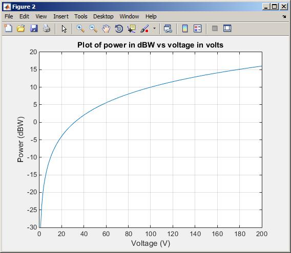
2.14 A program to calculate and plot the power consumed by a resistor as the voltage across the resistor is varied from 1 to 200 volts shown below:

© 2018 Cengage Learning®. All Rights Reserved. May not be scanned, copied or duplicated, or posted to a publicly accessible website, in whole or in part.

% Script file: p_resistor.m
%
% Purpose:
% To plot the power consumed by a resistor as a function
% of the voltage across the resistor on both a linear and % a log scale.
%
% Record of revisions:
% Date Programmer Description of change
% ==== ========== =====================
% 03/03/15 S. J. Chapman Original code
%
% Define variables:
% ir -- Current in the resistor (A)
% pr -- Power in the resistor (W)
% r -- Resistance of resistor (ohms)
% vr -- Voltage across the resistor (V)
% vr_db -- Voltage across the resistor (dBW)
% Set the resistance r = 1000;
% Create array of voltage across the resistor vr = 1:200;
% Calculate the current flow through the resistor ir = vr / r;
% Calculate the power consumed by the resistor in watts pr = ir .* vr;
% Calculate the power consumed by the resistor in dBW pr_db = 10 * log10(pr);
% Plot on linear scale figure(1); plot(vr,pr);
title('Plot of power in watts vs voltage in volts');
xlabel('Voltage (V)');
ylabel('Power (watts)'); grid on;
% Plot on semilog scale figure(2); plot(vr,pr_db);
title('Plot of power in dBW vs voltage in volts');
xlabel('Voltage (V)');
ylabel('Power (dBW)'); grid on;
The resulting plots are shown below.

2.15 (a) A program that accepts a 3D vector in rectangular coordinates and calculates the vector in spherical coordinates is shown below:
% Script file: rect2spherical.m
%
% Purpose:
% To calculate the spherical coordinates of a vector given
% the 3D rectangular coordinates.
%
% Record of revisions:
% Date Programmer Description of change
% ==== ========== =====================
% 03/04/15 S. J. Chapman Original code
%
% Define variables:
% x, y, z -- Rectangular coordinates of vector
% r -- Length of vector
% theta -- Direction of vector (x,y) plane, in degrees
% phi -- Elevation angle of vector, in degrees
% Prompt the user for the input points
x = input('Enter x: ');
y = input('Enter y: ');
z = input('Enter z: ');
% Calculate polar coordinates. Note that "180/pi" converts
% from radians to degrees.
r = sqrt(x^2 + y^2 + z^2); theta = atan2(y,x) * 180/pi; phi = atan2(z,sqrt(x^2 + y^2)) * 180/pi;
% Tell user disp ('The spherical coordinates are:'); disp (['r = ' num2str(r)]); disp (['theta = ' num2str(theta)]); disp (['phi = ' num2str(phi)]);
When this program is executed, the results are:
>> rect2spherical
Enter x: 4
Enter y: 3
Enter z: 0
The spherical coordinates are:
r = 5
theta = 36.8699
phi = 0
>> rect2spherical
Enter x: 4
Enter y: 0
Enter z: 3
The spherical coordinates are:
r = 5
theta = 0
phi = 36.8699
(b) A program that accepts a 3D vector in spherical coordinates (with the angles θ and ϕ in degrees) and calculates the vector in rectangular coordinates is shown below:
% Script file: spherical2rect.m
% % Purpose:
% To calculate the 3D rectangular coordinates of a vector
% given the spherical coordinates.
%
% Record of revisions:
% Date Programmer Description of change
% ==== ========== =====================
% 03/04/15 S. J. Chapman Original code
%
% Define variables:
% x, y, z -- Rectangular coordinates of vector
% r -- Length of vector
% theta -- Direction of vector (x,y) plane, in degrees
% phi -- Elevation angle of vector, in degrees
% Prompt the user for the input points
r = input('Enter vector length r: ');
theta = input('Enter plan view angle theta in degrees: ');
phi = input('Enter elevation angle phi in degrees: ');
% Calculate spherical coordinates. Note that "pi/180" converts
% from radians to degrees.
x = r * cos(phi * pi/180) * cos(theta * pi/180);
y = r * cos(phi * pi/180) * sin(theta * pi/180);
z = r * sin(phi * pi/180);
% Tell user disp ('The 3D rectangular coordinates are:');
disp (['x = ' num2str(x)]);
disp (['y = ' num2str(y)]);
disp (['z = ' num2str(z)]);
When this program is executed, the results are:
>> spherical2rect
Enter vector length r: 5
Enter plan view angle theta in degrees: 36.87
Enter elevation angle phi in degrees: 0
The rectangular coordinates are:
x = 4
y = 3
z = 0
>> spherical2rect
Enter vector length r: 5
Enter plan view angle theta in degrees: 0
Enter elevation angle phi in degrees: 36.87
The rectangular coordinates are:
x = 4
y = 0
z = 3
2.16 (a) A program that accepts a 3D vector in rectangular coordinates and calculates the vector in spherical coordinates is shown below:
% Script file: rect2spherical.m
%
% Purpose:
% To calculate the spherical coordinates of a vector given
% the 3D rectangular coordinates.
%
% Record of revisions:
% Date Programmer Description of change
% ==== ========== =====================
% 03/04/15 S. J. Chapman Original code
% 1. 03/04/15 S. J. Chapman Modified to use cart2sph
%
% Define variables:
% x, y, z -- Rectangular coordinates of vector
% r -- Length of vector
% theta -- Direction of vector (x,y) plane, in degrees
% phi -- Elevation angle of vector, in degrees
% Prompt the user for the input points
x = input('Enter x: ');
y = input('Enter y: ');
z = input('Enter z: ');
% Calculate polar coordinates. Note that "180/pi" converts
% from radians to degrees.
[theta,phi,r] = cart2sph(x,y,z);
theta = theta * 180/pi;
phi = phi * 180/pi;
% Tell user disp ('The spherical coordinates are:'); disp (['r = ' num2str(r)]); disp (['theta = ' num2str(theta)]); disp (['phi = ' num2str(phi)]);
When this program is executed, the results are:
>> rect2spherical
Enter x: 4
Enter y: 3
Enter z: 0
The spherical coordinates are:
r = 5
theta = 36.8699
phi = 0
>> rect2spherical
Enter x: 4
Enter y: 0
Enter z: 3
The spherical coordinates are:
r = 5
theta = 0
phi = 36.8699
(b) A program that accepts a 3D vector in spherical coordinates (with the angles θ and ϕ in degrees) and calculates the vector in rectangular coordinates is shown below:
% Script file: spherical2rect.m
% % Purpose:
% To calculate the 3D rectangular coordinates of a vector % given the spherical coordinates.
% % Record of revisions:
% Date Programmer Description of change
% ==== ========== =====================
% 03/04/15 S. J. Chapman Original code
% 1. 03/04/15 S. J. Chapman Modified to use sph2cart
%
% Define variables:
% x, y, z -- Rectangular coordinates of vector
% r -- Length of vector
% theta -- Direction of vector (x,y) plane, in degrees
% phi -- Elevation angle of vector, in degrees
% Prompt the user for the input points
r = input('Enter vector length r: ');
theta = input('Enter plan view angle theta in degrees: ');
phi = input('Enter elevation angle phi in degrees: ');
% Calculate spherical coordinates. Note that "pi/180" converts % from radians to degrees.
[x,y,z] = sph2cart(theta*pi/180,phi*pi/180,r);
% Tell user
disp ('The 3D rectangular coordinates are:'); disp (['x = ' num2str(x)]); disp (['y = ' num2str(y)]); disp (['z = ' num2str(z)]);
When this program is executed, the results are:
>> spherical2rect
Enter vector length r: 5
Enter plan view angle theta in degrees: 36.87
2.17
Enter elevation angle phi in degrees: 0
The rectangular coordinates are: x = 4
y = 3 z = 0
>> spherical2rect
Enter vector length r: 5
Enter plan view angle theta in degrees: 0
Enter elevation angle phi in degrees: 36.87
The rectangular coordinates are: x = 4 y = 0
z = 3
A program to calculate cosh(x) both from the definition and using the MATLAB intrinsic function is shown below. Note that we are using fprintf to display the results, so that we can control the number of digits displayed after the decimal point:
% Script file: cosh1.m
% % Purpose:
% To calculate the hyperbolic cosine of x.
%
% Record of revisions:
% Date Programmer Description of change % ==== ========== =====================
% 03/04/15 S. J. Chapman Original code %
% Define variables:
% x -- Input value
% res1 -- cosh(x) from the definition
% res2 -- cosh(x) from the MATLAB function
% Prompt the user for the input power. x = input('Enter x: ');
% Calculate cosh(x)
res1 = ( exp(x) + exp(-x) ) / 2; res2 = cosh(x);
% Tell user fprintf('Result from definition = %14.10f\n',res1); fprintf('Result from function = %14.10f\n',res2);
When this program is executed, the results are:
» cosh1 Enter x: 3
Result from definition = 10.0676619958
Result from function = 10.0676619958
A program to plot cosh x is shown below:
% Script file: cosh_plot.m
% % Purpose:
% To plot cosh x vs x.
%
% Record of revisions:
% Date Programmer Description of change
% ==== ========== =====================
% 03/04/15 S. J. Chapman Original code
%
% Define variables:
% x -- input values
% coshx -- cosh(x)
% Create array of power in input values x = -3:0.1:3;

% Calculate cosh(x) coshx = cosh(x);
% Plot on linear scale plot(x,coshx); title('Plot of cosh(x) vs x'); xlabel('x'); ylabel('cosh(x)'); grid on;
The resulting plot is shown below. Note that the function reaches a minimum value of 1.0 at x = 0.
2.18 A program to calculate the energy stored in a spring is shown below:
% Script file: spring.m
%
% Purpose:
% To calculate the energy stored in a spring.
% % Record of revisions:
% Date Programmer Description of change
% ==== ========== =====================
% 11/14/07 S. J. Chapman Original code
%
% Define variables:
% energy -- Stored energy (J)
% f -- Force on spring (N)
% k -- Spring constant (N/m)
% x -- Displacement (m)
% Prompt the user for the input force and spring constant. f = input('Enter force on spring (N): '); k = input('Enter spring constant (N/m): ');
% Calculate displacement x x = f/k;
% Calculate stored energy energy = 0.5 * k * x^2;
% Tell user
fprintf('Displacement = %.3f meters\n',x); fprintf('Stored energy = %.3f joules\n',energy);
When this program is executed, the results are as shown below. The second spring stores the most energy.
» spring
Enter force on spring (N): 20
Enter spring constant (N/m): 200
Displacement = 0.100 meters
Stored energy = 1.000 joules
» spring
Enter force on spring (N): 30
Enter spring constant (N/m): 250
Displacement = 0.120 meters
Stored energy = 1.800 joules
» spring
Enter force on spring (N): 25
Enter spring constant (N/m): 300
Displacement = 0.083 meters
Stored energy = 1.042 joules
» spring
Enter force on spring (N): 20
Enter spring constant (N/m): 800