Finite mathematics for business economics life sciences and social sciences 13th edition barnett sol by ngoc.hunter708

Finite Mathematics for Business Economics Life Sciences and Social Sciences 13th Edition Barnett Solutions Manual Visit to Download in Full: https://testbankdeal.com/download/finite-mathematics-for-bu siness-economics-life-sciences-and-social-sciences-13th-edition-barnett-solutions-ma nual/

10. The table specifies a function, since for each domain value there corresponds one and only one range value.

12. The table does not specify a function, since more than one range value corresponds to a given domain value.

(Range values 1, 2 correspond to domain value 9.)

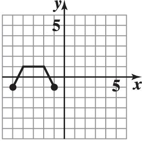
14. This is a function.

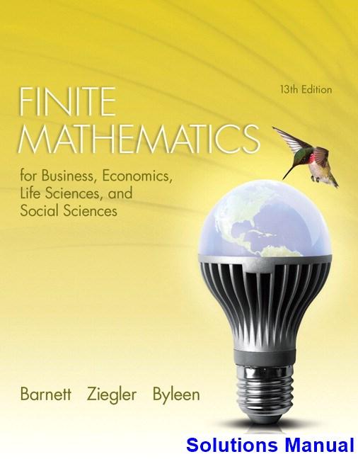
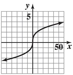
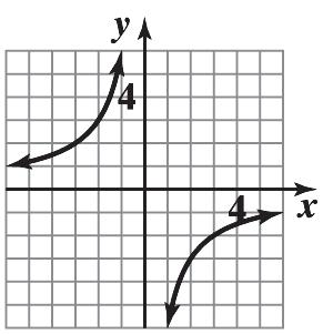
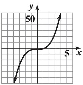
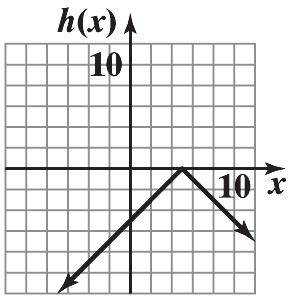
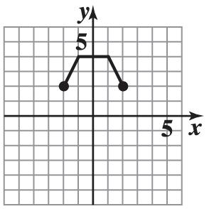
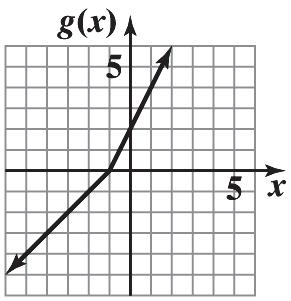
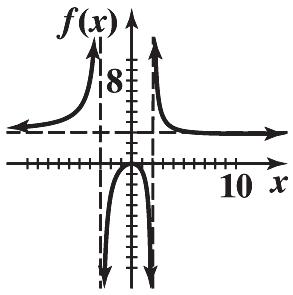
16. The graph specifies a function; each vertical line in the plane intersects the graph in at most one point.

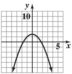
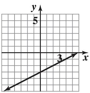
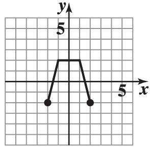
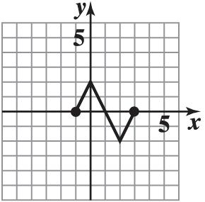
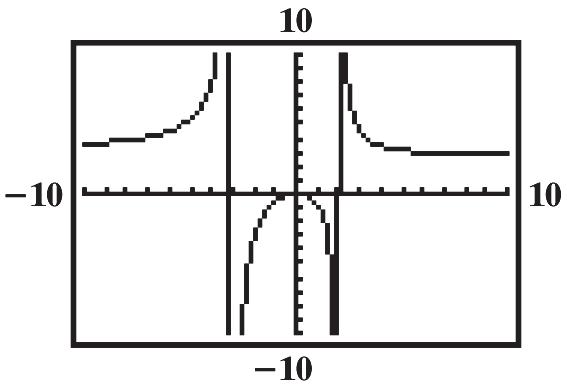
18. The graph does not specify a function. There are vertical lines which intersect the graph in more than one point. For example, the y-axis intersects the graph in two points.

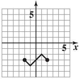
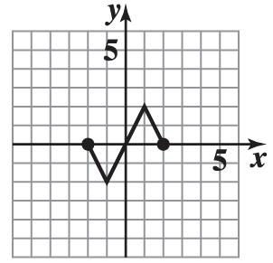
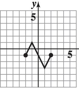
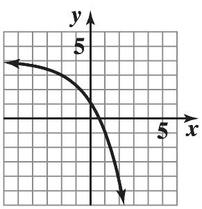
20. The graph does not specify a function.

EXERCISE 2-1 2-1

AND

GRAPHS EXERCISE 2-1

2. 4. 6. 8.

103 yx  is linear. 24. 2 8 xy is neither linear nor constant. 26. 2222 333333 which is consta. 3 t 4 n xxxx y    28. 9260 xy is linear. 30. 32. Finite Mathematics for Business Economics Life Sciences and Social Sciences 13th Edition Barnett Visit TestBankDeal.com to get complete for all chapters

22.

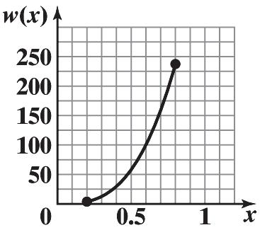
. Since the denominator is bigger than 1, we note that the values of f are between 0 and 3. Furthermore, the function f has the property that f(–x) = f(x). So, adding points x = 3, x = 4,

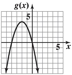
. Solving for y we have:

This equation specifies a function. The domain is R, the set of real numbers.

. Solving for y we have:

This equation specifies a function. The domain is all real numbers except 0.

Solving for y we have:

This equation does not define y as a function of x. For example, when x = 0, y=

. Solving for y we have: 31/6 and.

 

This equation specifies a function. The domain is all nonnegative real numbers, i.e., 0 x

2-2 CHAPTER 2 FUNCTIONS AND GRAPHS

34. 36.

x 

x –5 –4 –3 –2 –1 0 1 2 3 4 5 F(x) 2.78 2.67 2.45 2 1 0 1 2 2.45 2.67 2.78

38. f(x) = 2 2 3 2 x

= 5, we have:

42.

44.

46.

48.

50.

52. 5 x  54.

6721 xy

6 7216and3. 7 yxyx 

The sketch is: 40. y = f(4) = 0

y = f(–2) = 3

= 3, x < 0 at x = –4, –2

f(x) = 4 at x = 5

All real numbers

All real numbers except x = 2

Given



2 2 4 4and. x xyxy x  

56. Given ()4xxy

58.

22 9. xy

222 9and 9.yxyx 

Given





3. 60. Given 3 0 xy

yxyx

 62. 2 (5)(5)425421 f  64. 222 (2)(2)44444 fxxxxxx  66. 22 (10)(10)41004 fxxx 68.  2 ()44 fxxx 70. 2222 (3)()(3)44541 ffhhhh  72. (3)(3)496456222 fhhhhhh  74. (3)(3)(3)4(3)4(964)(94)62222 fhfhhhhh   

82. Given A =  w = 81.

Thus, w = 81

. Now P = 2

The domain is  > 0.

84. Given P = 2  + 2w = 160 or  + w = 80 and  = 80 – w.

Now A =  w = (80 – w)w and A = 80w–w 2

The domain is 0 < w< 80. [Note: w < 80 since w  80 implies   0.]

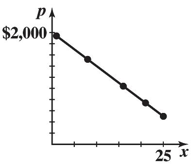
86. (A)

(B) p(11) = 1,340 dollars per computer p(18) = 920 dollars per computer

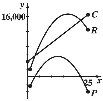
88. (A) R(x) = xp(x) = x(2,000 – 60x) thousands of dollars

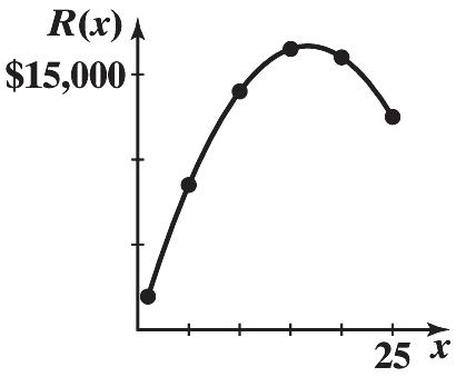
Domain: 1 ≤ x ≤ 25

(B) Table 11 Revenue

EXERCISE 2-1 2-3 Copyright

76. (A) ()3()9339 fxhxhxh  (B)     ()()339393 fxhfxxhxh  (C) ()()3 3 fxhfxh hh   78. (A) 2 22 22 ()3()5()8 3(2)558 363558 fxhxhxh xxhhxh xxhhxh    (B)     222 2 ()()363558358 635 fxhfxxxhhxhxx xhhh   (C) 2

hh   80. (A)

h 

()()635 635fxhfxxhhhxh

f(x + h) = x 2 + 2xh + h2 + 40x + 40h (B) f(x + h) – f(x) = 2xh + h2 + 40h (C) ()() fxhfx

= 2x + h + 40

2  + 2 81      = 2  + 162  .



w =

x(thousands) R(x)(thousands) 1 $1,940 5 8,500 10 14,000 15 16,500 20 16,000 25 12,500 (C)

90. (A) P(x) = R(x) – C(x)

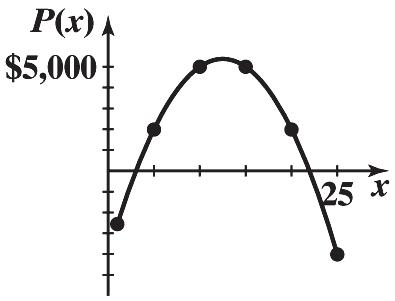
= x(2,000 – 60x) – (4,000 + 500x) thousand dollars

= 1,500x – 60x 2 – 4,000

Domain: 1 ≤ x ≤ 25

(B) Table 13 Profit

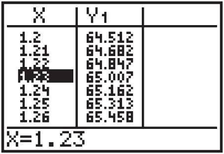
92. (A) 1.2 inches

(B) Evaluate the volume function for x = 1.21, 1.22, …, and choose the value of x whose volume is closest to 65.

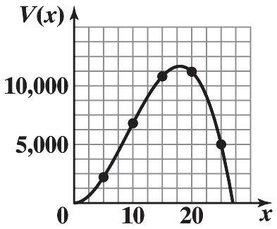
94. (A) V(x) = x 2 (1084) x

(B) 0 < x < 27

96. (A) Given 5v – 2s = 1.4. Solving for v, we have:

v = 0.4s + 0.28.

If s = 0.51, then v = 0.4(0.51) + 0.28 = 0.484 or 48.4%.

(B) Solving the equation for s, we have: s = 2.5v – 0.7.

If v = 0.51, then s = 2.5(0.51) – 0.7 = 0.575 or 57.5%.

EXERCISE 2-2

2. ()412fxx Domain: all real numbers; range: all real numbers.

4. ()3 fxx  Domain: [0,)  ; range: [3,)  .

6. ()52fxx Domain: all real numbers; range: (,2]. 

2-4

CHAPTER 2 FUNCTIONS AND GRAPHS

x (thousands) P

(thousands) 1 –$2,560 5 2,000 10 5,000 15 5,000 20 2,000 25 –4,000 (C)

(x)

x V(x) 5 2,200 10 6,800 15 10,800 20 11,200 25 5,000 (D)

8. 3 ()2010 fxx  Domain: all real numbers; range: all real numbers.

EXERCISE 2-2 2-5

10. 12. 14. 16. 18.

22.

20.

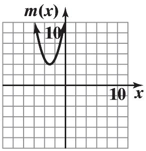
26. The graph of h(x) = –|x – 5| is the graph of y = |x| reflected in the x axis and shifted 5 units to the right. 24. 28. The graph of m(x) = (x + 3)2 + 4 is the graph of y = x 2 shifted 3 units to the left and 4 units up.

30. The graph of g(x) = –6 + 3 x is the graph of y = 3 x shifted 6 units down.

32. The graph of m(x) = –0.4x 2 is the graph of y = x 2 reflected in the x axis and vertically contracted by a factor of 0.4.

34. The graph of the basic function y = |x| is shifted 3 units to the right and 2 units up. y = |x – 3| + 2

36. The graph of the basic function y = |x| is reflected in the x axis, shifted 2 units to the left and 3 units up.

Equation: y = 3 – |x + 2|

38. The graph of the basic function 3 x is reflected in the x axis and shifted up 2 units. Equation: y = 2 – 3 x

40. The graph of the basic function y = x 3 is reflected in the x axis, shifted to the right 3 units and up 1 unit.

Equation: y = 1 – (x – 3)3

2-6 CHAPTER 2 FUNCTIONS AND GRAPHS

42. g(x) = 3 3 x  + 2 44. g(x) = –|x – 1| 46. g(x) = 4 – (x + 2)2 48. g(x) = 1if 1 22if 1 xx xx      50. h(x) = 102if020 400.5if20 xx xx     

54. The graph of the basic function y = x is reflected in the x axis and vertically expanded by a factor of 2. Equation: y = –2x

56. The graph of the basic function y = |x| is vertically expanded by a factor of 4. Equation: y = 4|x|

58. The graph of the basic function y = x 3 is vertically contracted by a factor of 0.25. Equation: y = 0.25x 3 .

60. Vertical shift, reflection in y axis.

Reversing the order does not change the result. Consider a point (a,b) in the plane. A vertical shift of k units followed by a reflection in y axis moves (a,b) to (a, b + k) and then to (–a, b + k). In the reverse order, a reflection in y axis followed by a vertical shift of k units moves (a,b) to (–a,b) and then to (–a,b + k). The results are the same.

62. Vertical shift, vertical expansion.

Reversing the order can change the result. For example, let (a,b) be a point in the plane. A vertical shift of k units followed by a vertical expansion of h (h > 1) moves (a,b) to (a,b + k) and then to (a,bh + kh). In the reverse order, a vertical expansion of h followed by a vertical shift of k units moves (a,b) to (a,bh) and then to (a,bh + k); (a,bh + kh) ≠ (a,bh + k).

64. Horizontal shift, vertical contraction.

Reversing the order does not change the result. Consider a point (a,b) in the plane. A horizontal shift of k units followed by a vertical contraction of h (0 < h < 1) moves (a,b) to (a + k,b) and then to (a + k,bh). In the reverse order, a vertical contraction of h followed by a horizontal shift of k units moves (a,b) to (a,bh) and then to (a + k,bh). The results are the same.

66. (A) The graph of the basic function y = x is vertically expanded by a factor of 4.

68. (A) The graph of the basic function y = x 2 is reflected in the x axis, vertically contracted by a factor of 0.013, and shifted 10 units to the right and 190 units up.

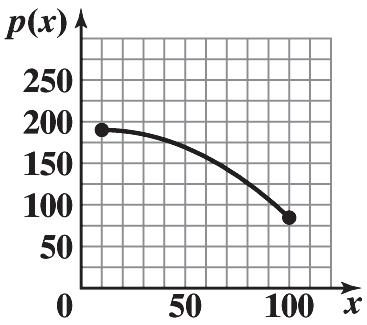
(B) (B)

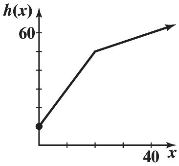
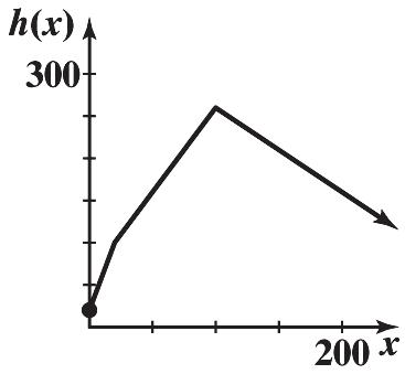
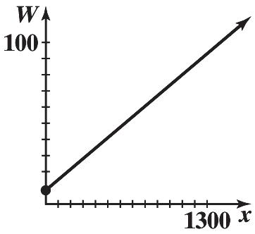
70. (A) Let x = number of kwh used in a winter month. For 0 ≤ x ≤ 700, the charge is 8.5 + .065x. At x = 700, the charge is $54. For x > 700, the charge is 54 + .053(x – 700) = 16.9 + 0.053x. Thus,

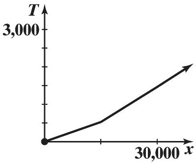
72. (A) Let x = taxable income.

If 0 ≤ x ≤ 15,000, the tax due is $.035x. At x = 15,000, the tax due is $525. For 15,000 < x ≤ 30,000, the tax due is 525 + .0625(x – 15,000) = .0625x –

(B)        

(x) = 0.035if 015,000 0.0625412.5 if 15,00030,000 0.0645472.5if 30,000

T(35,000) = $1,785

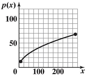
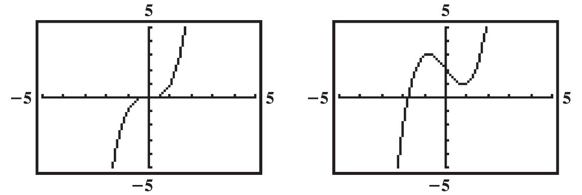
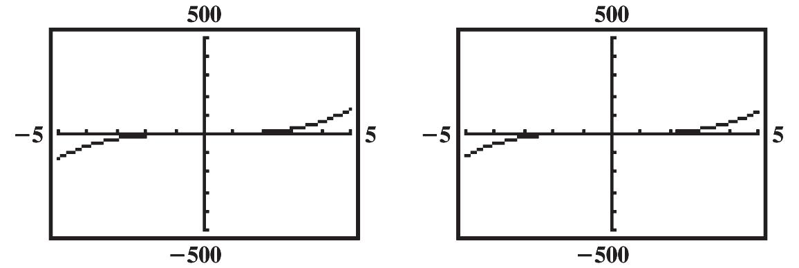
74. (A) The graph of the basic function y = x 3 is vertically expanded by a factor of 463.

76. (A) The graph of the basic function y = 3 x is reflected in the x axis and shifted up 10 units.

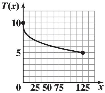
(B) (B)

2 16 xx 

(12)8 xx

2-8 CHAPTER 2 FUNCTIONS AND GRAPHS

W(x)

8.5.065if

16.90.053if

xx xx      (B)

0700

700

412.5. For x > 30,000, the tax due is 1,462.5 + .0645(x –30,000) = .0645x – 472.5. Thus, xx xx xx

EXERCISE 2-3 2.

(standard form) 4. 2 128

(standard form)

 

(8)64 x

(1236)836 xx

2 6464 16 xx

(completing the square) 2

 (vertex form) 2

(completing the square)

2 (6)44

(vertex form)

6. 2 31821 xx (standard form)

3(6)21

3(699)21(completing the square)

3(3)2127

2 2 2 2

3(3)6(vertex form)

x xx x  

5()11 5()11(completing the square) 5() (vertex form)

3 3 11 5()

x x

99 44 345 24 2 3 1 24



12. The graph of n(x) is the graph of y = x 2 reflected in the x axis, then shifted right 4 units and up 7 units; 2 ()(4)7.nxx

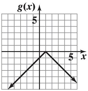
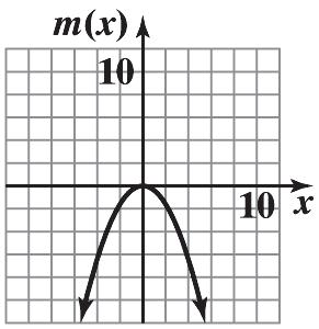
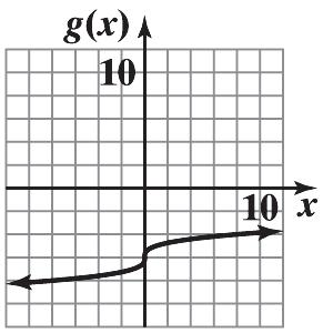
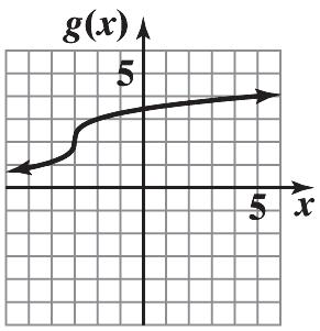
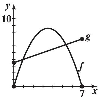
14. (A) g (B) m (C) n (D) f

16. (A) x intercepts: –5, –1; y intercept: –5 (B) Vertex: (–3, 4)

18. (A) x intercepts: 1, 5; y intercept: 5 (B) Vertex: (3, –4)

20. g(x) = –(x + 2)2 + 3

(

x + 2)2 = 3

(B) Vertex: (–2, 3) (C) Maximum: 3 (D) Range: y ≤ 3 or (–∞, 3]

22. n(x) = (x – 4)2 – 3

–

– 4

= 4 – 3 , 4 + 3

(B) Vertex: (4, –3) (C) Minimum: –3 (D) Range: y ≥ –3 or [–3, ∞)

EXERCISE 2-3 2-9

  

x x 

8. 2 51511 xx  (standard form) 2 2 2

10. The graph of g(x) is the graph of y = x 2 shifted right 1 unit and down 6 units; 2 ()(1)6.gxx

x +

x =

(A) x intercepts: –(x + 2)2 + 3 = 0

2 =

–2 – 3 , –2 + 3

y intercept: –1

= ±

(A) x intercepts: (x – 4)2 – 3 = 0

4)2 = 3

y intercept: 13

2-10

CHAPTER 2 FUNCTIONS AND GRAPHS

24. y = –(x – 4)2 + 2 26. y = [x – (–3)]2 + 1 or y = (x + 3)2 + 1 28. g(x) = x 2 – 6x + 5 = x 2 – 6x + 9 – 4 = (x – 3)2 – 4 (A) x intercepts: (x – 3)2 – 4 = 0 (x – 3)2 = 4 x – 3 = ±2 x = 1, 5 y intercept: 5 (B) Vertex: (3, –4) (C) Minimum: –4 (D) Range: y ≥ –4 or [–4, ∞) 30. s(x) = –4x 2 – 8x – 3 = –4 2 3 2 4 xx     = –4 2 1 21 4 xx        = –4 2 1 (1) 4 x        = –4(x + 1)2 + 1 (A) x intercepts: –4(x + 1)2 + 1 = 0 4(x + 1)2 = 1 (x + 1)2 = 1 4 x + 1 = ± 1 2 x = –3 2 , –1 2 y intercept: –3 (B) Vertex: (–1, 1) (C) Maximum: 1 (D) Range: y ≤ 1 or (–∞, 1] 32. v(x) = 0.5x 2 + 4x + 10 = 0.5[x 2 + 8x + 20] = 0.5[x 2 + 8x + 16 + 4] = 0.5[(x + 4)2 + 4] = 0.5(x + 4)2 + 2 (A) x intercepts: none y intercept: 10 (B) Vertex: (–4, 2) (C) Minimum: 2 (D) Range: y ≥ 2 or [2, ∞) 34. g(x) = –0.6x 2 + 3x + 4 (A) g(x) = –2: –0.6x 2 + 3x + 4 = –2 0.6x 2 – 3x – 6 = 0 x = –1.53, 6.53 (B) g(x) = 5: –0.6x 2 + 3x + 4 = 5 –0.6x 2 + 3x – 1 = 0 0.6x 2 – 3x + 1 = 0 x = 0.36, 4.64

–0.6x 2 + 3x – 4 = 0

x 2 – 3x + 4 = 0

No solution

36. Using a graphing utility with y = 100x – 7x 2 – 10 and the calculus option with maximum command, we obtain 347.1429 as the maximum value.

38. m(x) = 0.20x 2 – 1.6x – 1 = 0.20(x 2 – 8x – 5) = 0.20[(x – 4)2 – 21] = 0.20(x – 4)2 – 4.2

(A) x intercepts: 0.20(x – 4)2 – 4.2 = 0 (

– 4)2 = 21

x – 4 = ± 21

x = 4 – 21 = –0.6, 4 + 21 = 8.6;

intercept: –1

(A) x intercepts:

x + 3)2 + 4.65 = 0

x + 3)2 = 31 x + 3 = ± 31

EXERCISE 2-3 2-11

0.6

Minimum:

40. n(x)

–0.15

3.3

–0.15(x 2 + 6x – 22) = –0.15[(x + 3)2 – 31] = –0.15(x + 3)2 + 4.65

(B) Vertex: (4, –4.2) (C)

–4.2 (D) Range: y ≥ –4.2 or [4.2,) 

x 2 – 0.90

–0.15(

Maximum:

42. x = –1.27, 2.77 44. –0.88 ≤ x ≤ 3.52 46. x < –1 or x > 2.72

(

x = –3 – 31 = –8.6,–3 + 31 = 2.6; y intercept: 3.30 (B) Vertex: (–3, 4.65) (C)

4.65 (D) Range: x ≤ 4.65 or (,4.65] 

48. f is a quadratic function and max f(x) = f(–3) = –5

Axis: x = –3

Vertex: (–3, –5)

x intercepts: None

56.

58.

2-12

CHAPTER 2 FUNCTIONS AND GRAPHS

Range: y ≤ –5 or (–∞, –5]

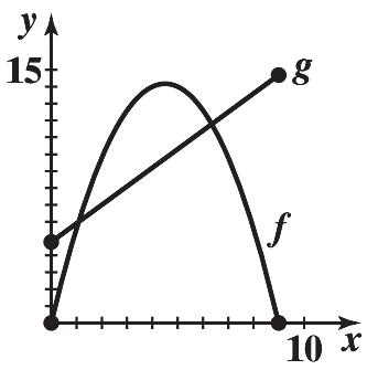
50. (A) (B) f(x) = g(x): –0.7x(x – 7) = 0.5x + 3.5 –0.7x 2 + 4.4x – 3.5 = 0 x = 2 4.4(4.4)4(0.7)(3.5) 1.4  = 0.93, 5.35 (C) f(x) > g(x) for 0.93 < x < 5.35 (D) f(x) < g(x) for 0 ≤ x < 0.93 or 5.35 < x ≤ 7 52. (A) (B) f(x) = g(x): –0.7x 2 + 6.3x = 1.1x + 4.8 –0.7x 2 + 5.2x – 4.8 = 0 0.7x 2 – 5.2x + 4.8 = 0 x =  2 5.2(5.2)4(0.7)(4.8) 1.4  = 1.08, 6.35 (C) f(x) > g(x)

1.08

6.35

f(x) < g(x) for 0 ≤ x < 1.08 or 6.35 < x ≤ 9

for

< x <

(D)

–axis.

54. A quadratic with no real zeros will not intersect the x



Such an equation will have 2 40.bac



Such an equation will have 0. k a

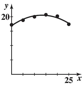
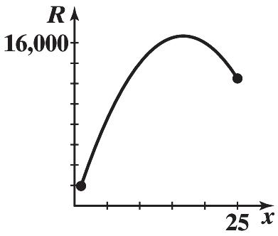
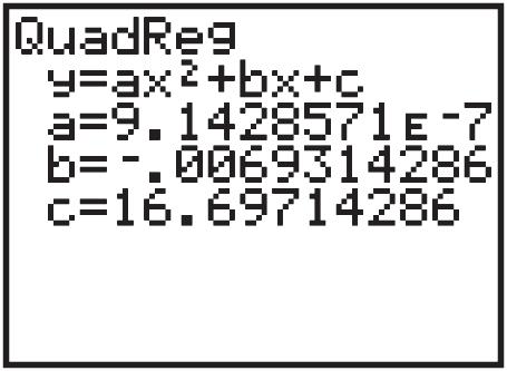
EXERCISE 2-3 2-13 Copyright © 2015 Pearson Education, Inc. 60. 22 22 22 () (2) 2 axbxcaxhk axhxhk axahxahk    Equating constant terms gives 2 kcah  . Since h is the vertex, we have 2 b h a  . Substituting then gives 2 4 4 kcah acb a   f(x) = –0.0169x 2 + 0.47x + 17.1 (A) Mkt Share() 017.217.1 518.819.0 1020.020.1 1520,720.3 2020.219.7 2517.418.3 3016.416.0 xfx (B) (C) For 2020, x = 40 and f(40) = –0.0169(30)2 + 0.47(40) + 17.1 = 8.9% For 2025, x = 45 and f(45) = –0.0169(45)2 + 0.47(45) + 17.1 = 4.0% (D) Market share rose from 17.2% in 1980 to a maximum of 20.7% in 1995 and then fell to 16.4% in 2010. 64. Verify 66. (A) (B) R(x) = 2,000x – 60x 2 = 2 100 60 3 xx    = 2 10025002500 60 399 xx        = 2 502500 60 39 x            = 2 50 60 3 x    + 50,000 3 16.667 thousand computers(16,667 computers); 16,666.667 thousand dollars ($16,666,667)

200060(50/3) $1,000

(C)

(B) R(x) = C(x)

x(2,000 – 60x) = 4,000 + 500x 2,000x – 60x 2 = 4,000 + 500x 60x 2 – 1,500x + 4,000 = 0

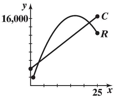
6x 2 – 150x + 400 = 0

x = 3.035, 21.965

Break-even at 3.035 thousand (3,035) and 21.965 thousand (21,965)

(B) and (C) Intercepts and break-even points: 3,035 computers and 21,965 computers

(D) and (E) Maximum profit is $5,375,000 when 12,500 computers are produced. This is much smaller than the maximum revenue of $16,666,667. 72.

For x = 2,300, the estimated fuel consumption is y = a(2,300)2 + b(2,300) + c = 5.6 mpg.

2-14 CHAPTER 2 FUNCTIONS

AND GRAPHS

 

2,000

60 50 3    = $1,000

68. (A)

50 3 

–

70. (A) P(x) = R(x) – C(x) = 1,500x – 60x 2 – 4,000

Solve:

(

1,000(0.04

40 – 1000x 2 = 30 1000x 2 = 10 x 2 = 0.01 x = 0.10 cm 40 00.2 0

x) =

– x2) = 30

74.

()7212 fxx 

EXERCISE 2-4 2.

(A) Degree: 1



x x x  

x-intercept: x= –6

y-intercept: 72

4. 3 ()(5)fxxx

(A) Degree: 4

(B) 3 (5)0 0,5 xx x  

x-intercepts: 0,5

y-intercept: 0

6. 2 ()45 fxxx

(A) Degree: 2

(B) (5)(1)0 1,5 xx x  

x-intercepts: –1, 5

y-intercept: –5

8. 23 ()(4)(27) fxxx

(A) Degree: 5

(B) 23 (4)(27)0 xx 2,2,3 x 

x-intercepts: 2,2,3 x 

y-intercept: –108

10. 26 ()(3)(84) fxxx

(A) Degree: 8

(B)  (3)840 xx

1 2 3, x 

x-intercepts: 3,1/2

EXERCISE 2-4 2-15

(B) 72120 1272 6

y-intercept: 36,864

12. (A) Minimum degree: 2

(B) Negative – it must have even degree, and positive values in the domain are mapped to negative values in the range.

14. (A) Minimum degree: 3

(B) Negative – it must have odd degree, and positive values in the domain are mapped to negative values in the range.

16. (A) Minimum degree: 4

(B) Positive – it must have even degree, and positive values in the domain are mapped to positive values in the range.

18. (A) Minimum degree: 5

(B) Positive – it must have odd degree, and positive values in the domain are mapped to positive values in the range.

20. A polynomial of degree 7 can have at most 7 x-intercepts.

22. A polynomial of degree 6 may have no x intercepts. For example, the polynomial 6 ()1fxx has no x- intercepts.

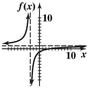
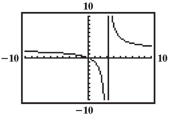
24. (A) Intercepts:

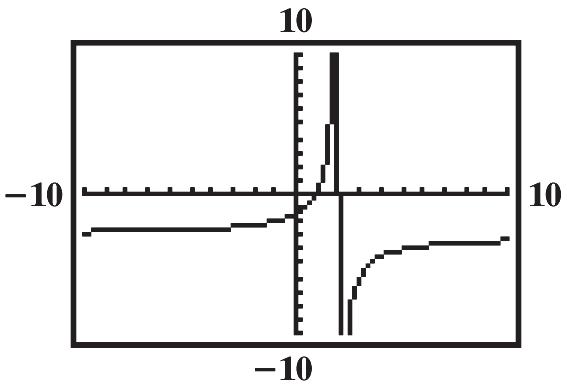
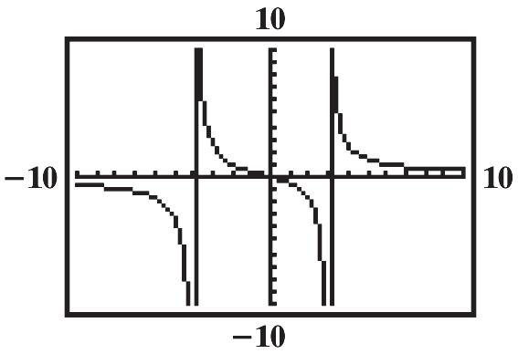
(B) Domain: all real numbers except x = –3

(C) Vertical asymptote at x = –3 by case 1 of the vertical asymptote procedure on page 90. Horizontal asymptote at y = 1 by case 2 of the horizontal asymptote procedure on page 90.

(D) (E)

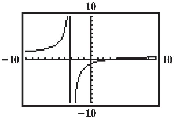
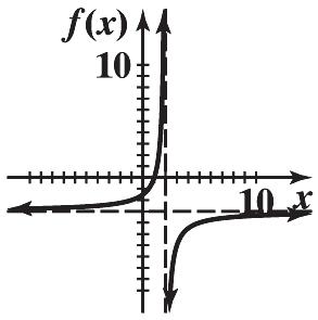
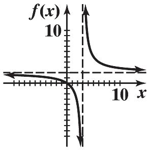
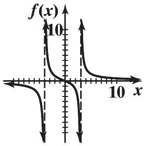
26. (A) Intercepts:

(B) Domain: all real numbers except x = 3.

(C) Vertical asymptote at x = 3 by case 1 of the vertical asymptote procedure on page 90. Horizontal asymptote at y = 2 by case 2 of the horizontal asymptote procedure on page 90.

2-16 CHAPTER 2 FUNCTIONS

AND GRAPHS

x-intercept(s): 30 3 x x   (3, 0) y-intercept: 03 (0)1 03 f   (0, –1)

-intercept(s): 20 0 x x   (0, 0) y-intercept: 2(0) (0)0 03 f  (0, 0)

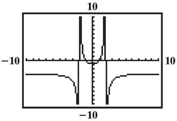
(B) Domain: all real numbers except 2 x 

(C) Vertical asymptote at x = 2 by case 1 of the vertical asymptote procedure on page 90. Horizontal asymptote at y = –3 by case 2 of the horizontal asymptote procedure on page 90.

EXERCISE 2-4 2-17

(E)

(D)

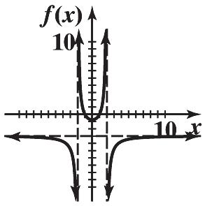
28. (A) Intercepts:

(E) 30. (A) (B) x-intercept: 330 1 x x   (1, 0) y-intercept: 33(0)3 (0) 022 f  3 0, 2    

(D)

34. 6 4 y  , by case 2 for horizontal asymptotes on page 90.

36. 1 2 y  , by case 2 for horizontal asymptotes on page 90.

38. 0 y  , by case 1 for horizontal asymptotes on page 90.

40. No horizontal asymptote, by case 3 for horizontal asymptotes on page 90.

42. Here we have denominator 22 (4)(16)(2)(2)(4)(4) xxxxxx  . Since none of these linear terms are factors of the numerator, the function has vertical asymptotes at x = 2, x = –2, x = 4, and x = –4.

44. Here we have denominator 2 78(1)(8)xxxx  . Also, we have numerator

2 87(1)(7)xxxx  . By case 2 of the vertical asymptote procedure on page 90, we conclude that the function has a vertical asymptote at x = –8.

46. Here we have denominator 32232(32)(2)(1) xxxxxxxxx  . We also have numerator

2 2(2)(1)xxxx  . By case 2 of the vertical asymptote procedure on page 90, we conclude that the function has a vertical asymptotes at x = 0 and x = 2.

48. (A) Intercepts:

(B) Vertical asymptote when 2 6(2)(3)0xxxx ; so, vertical asymptotes at x = 2, x = –3. Horizontal

2-18 CHAPTER 2 FUNCTIONS AND GRAPHS

32. (A) (B)

asymptote 3

x-intercept(s): 2 30 0 x x   (0, 0) y-intercept: (0)0 f  (0, 0)

y 

(C)

50. (A) Intercepts:

Vertical asymptotes when 2 40 x  ; i.e. at x = 2 and x = –2. Horizontal asymptote at 3 y  (C) (D) 52. (A) Intercepts:

12(4)(3)0xxxx

EXERCISE 2-4 2-19

(B)



(D) x-intercept(s): 2 2 1 330 33 x x x    (1,0), (–1,0) y-intercept: 3 (0) 4 f  3 0, 4    x-intercept(s): 5100 2 x x   (2,0) y-intercept: 105 (0) 126 f  (0,5/6)

(B) Vertical asymptote when

; i.e. when x = – 4 and when x = 3. Horizontal asymptote at y = 0. (C)

54. 2 ()(2)(1)2 fxxxxx 

()(1)(1)123 fxxxxxxxx 

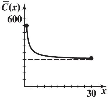
58. (A) We want () Cxmxb  . Fixed costs are $300 b  per day. Given (20)5,100 C  we have

(B)

(D) Average cost tends towards $240 as production increases.

2-20 CHAPTER 2 FUNCTIONS AND

GRAPHS



56. 

(20)3005,100 204800 240 ()240300 m m m Cxx    

()240()240300300 Cxx Cx xxx   (C)

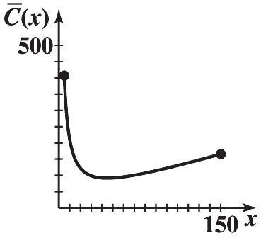
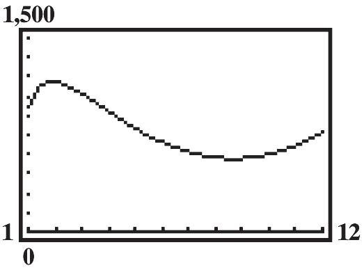
60. (A) 2 22,000 () xx Cx x   (B)

62. (A) 32 203602,3001,000

(B)

64. (A)

(B) (42)156 y

eggs

66. (A) The horizontal asymptote is y = 55.

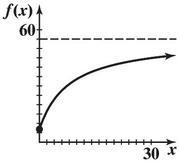
(B)

68. (A)

(B) This model gives an estimate of 2.5 divorces per 1,000 marriages.

EXERCISE 2-5

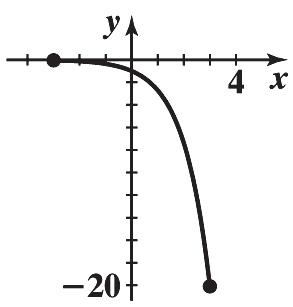
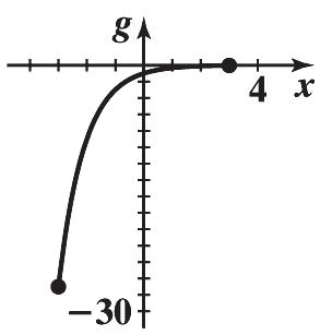
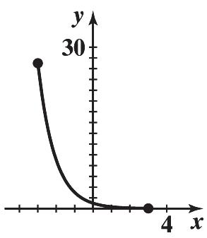
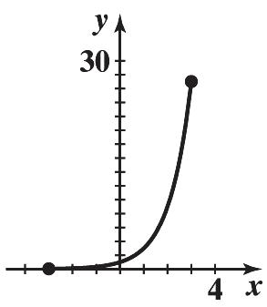
2. A. graph g B. graph f C. graph h D. graph k

EXERCISE 2-5 2-21

() xxx Cx x  



12. The graph of g is the graph of f shifted 2 units to the right.

14. The graph of g is the graph of f reflected in the x axis.

16. The graph of g is the graph of f shifted 2 units down.

18. The graph of g is the graph of f vertically contracted by a factor of 0.5 and shifted 1 unit to the right.

20. A. ()2yfx B. (3)yfx

2-22 CHAPTER 2

FUNCTIONS AND GRAPHS

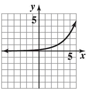
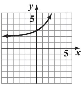
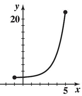
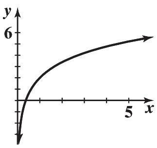
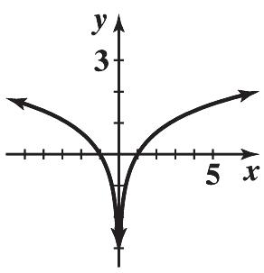
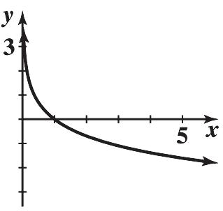
4 3;[3,3] x y  xy –3 1 27 –1 1 3 0 1 1 3 3 27 6. 3;[3,3] x y  xy –3 27 –1 3 0 1 1 1 3 3 1 27 8. ()3;[3,3] x gx  x ()gx –3 –27 –1 –3 0 –1 1 1 3 3 1 27 10 ;[3,3] x ye xy –3 0.05 –1 0.37 0 –1 1 2.72 3 20.09



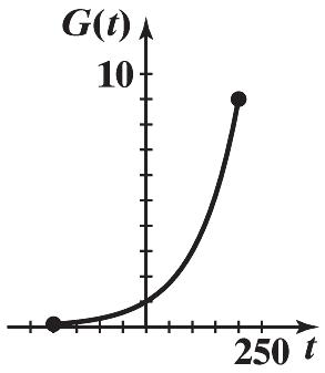
EXERCISE 2-5 2-23

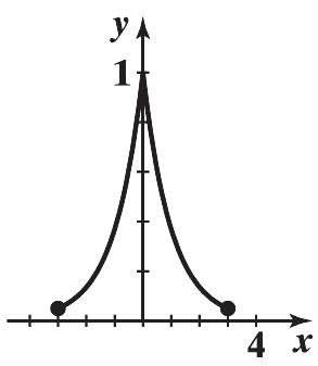
C. 2()4yfx D. 4(2)yfx 22. 100 ()3;[200,200]Gtt x ()Gt –200 1 9 –100 1 3 0 1 100 3 200 9 24. 2 2;[1,5] x ye xy –1 2.05  0 2.14  1 2.37  3 4.72  5 22.09  26. ;[3,3] x ye xy –3 0.05  –1 0.37  0 1 1 0.37  3 0.05  28. 2, a  2 b  for example. The exponential function property: For 0, x  xxab  if and only if ab  assumes 0 a  and 0. b  30. 55342 342 2 2 xx xx x x     32. 2 23 2 2 77 23 230 (3)(1)0 1,3 xx xx xx xx x       34. 55 (1)(21) 121 32 2 3 xx xx x x     36. 1050 e(105)0 1050(since 0) 1/2 xx x x xee x xe x     38. 2 2 2 90 (9)0 (9)0(since 0) 3,3 xx x x xee ex xe x     40. 4 4 0for all ; 0has no solutions. x x eex ee   42. 31 311 0 311 2/3 x x ee ee x x    

CHAPTER 2 FUNCTIONS AND GRAPHS

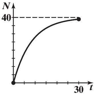
The maximum number of boards an average employee can be expected to produce in 1 day is 40.

(A) The average salary in 2022: (32) y  $20,186,000.

(B) The model gives an average salary of (7) y  $1,943,000 in 1997.

2-24

44. ()(3);[0,3] x mxx  x ()mx 0 0 1 1 3 2 2 9 3 1 9 46. 200 ;[0,5] 13 t N e   xN 0 50 1 95.07  2 142.25  3 174.01  4 ≈ 189.58 5 196.04  48. (0.0435)(7) 0.3045 (24,000) (24,000) (24,000)(1.35594686) $32,542.72 rt APe Ae Ae A A      50. (A) (52)(0.5) 0.06 52 26 (1) 4000(1) 4000(1.0011538462) 4000(1.030436713) $4121.75 rmt m AP A A A A      (B) (52)(10) 0.06 52 520 (1) 4000(1) 4000(1.0011538462) 4000(1.821488661) $7285.95 rmt m AP A A A A      52. (365)(17) 0.055 365 6205 (1) 40,000(1) 40,000(1.0001506849) 40,000(2.547034043) $15,705 rmt m AP P P P P      54. (A) (4)(5) 0.0135 4 20 (1) 10,000(1) 10,000(1.003375) 10,000(1.069709) $10,697.09 rmt m AP A A A A      (B) (12)(5) 0.0130 12 60 (1) 10,000(1) 10,000(1.00108333) 10,000(1.067121479) $10,671.21 rmt m AP A A A A      (C) (365)(5) 0.0125 365 1825 (1) 10,000(1) 10,000(1.000034247) 10,000(1.06449332) $10,644.93 rmt m AP A A A A      56. 0.12 40(1);[0,30]Net  xN 0 0 10 27.95  20 36.37  30 38.91 

58.

expectancy for a person born in 2025: (55)81.5

36. False; an example of a polynomial function of odd degree that is not one–to–one is 3 ().

fxxx

38. True; the graph of every function (not necessarily one–to–one) intersects each vertical line exactly once.

40. False; 1 x is in the domain of f, but cannot be in the range of g.

42. True; since g is the inverse of f, then (a, b) is on the graph of f if and only if (b, a) is on the graph of g

Therefore, f is also the inverse of g.

EXERCISE 2-6 2-25

60. (A) 0.00942(50) (50)62 o IIe % (B) 0.00942(100) (100)39 o IIe % 62. (A) 0.032 94.Pet  (B) Population in 2025: 0.032(13) (13)94142,000,000;Pe Population in 2035: 0.032(23) (23)94196,000,000Pe . 64. Life

y 

EXERCISE 2-6 2. 5 2 log325322    4. 0 log101 ee    6. 3 2 9 3 log27279 2    8. 2 6 366log362    10. 2 3 27 2 927log9 3    12. log x MbbMx    14. 5 1010 log100,000log105  16. 1 1 33 3 loglog31  18. 0 44 log1log40  20. 5 lne5  22. logloglog  bbb FGFG 24. 15 log15log  bbww 26. 3 3 log log log  R P P R 28. 2 2 log2 2 4    x x x 30. 3 3 log27 327 33 3     y y y y 32. 2 22 log2    be eb eb 34. 1 2 25 1 log 2 25 5    x x x

years.



(1)(0)(1)0. fff

44. 2 2 3 2 loglog272log2log3 3 loglog27log2log3 loglog9log4log3 (9)(4) loglog 3 loglog12 12       bbbb bbbb bbbb bb bb x x x x x x 46. 1 3 2 1 log3log2log25log20 2 loglog2log25log20 loglog8log5log20 (8)(5) loglog 20 loglog2 2       bbbb bbbb bbbb bb bb x x x x x x

Since the domain of a logarithmic function is (0,),  omit the negative solution. Therefore, the

shifted to the left 2 units. 56. The domain of logarithmic function is defined for positive values only. Therefore, the domain of the function is

x or 1.

x The range of a logarithmic function is all real numbers. In interval notation the domain is (1,)

and the range is (,).

2-26 CHAPTER 2 FUNCTIONS AND GRAPHS

48. 2 2 2 log(2)loglog24 log(2)log24 log(2)log24 224 2240 (6)(4)0 6,4        bbb bb bb xx xx xx xx xx xx x

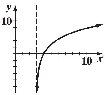
4.  x 50. 1010 10 1 log(6)log(3)1 6 log1 3 6 10 3 10(3)6 10306 4         xx x x x x xx xx x 52. 3 log(2) 32 32    y y yx x x xy 53 27 3 17 9 2 5 3 1 1 0 1 1 7 2 25 3 54. The graph of 3 log(2)yx is the graph of 3 log  yx

10

 58. A. log72.6041.86096  B. log0.0330411.48095  C. ln40,25710.60304  D. ln0.00592635.12836  60. A. 12.0832 log2.0832 log(2.0832)10 121.1156 x x x    B. 11.1577 log1.1577 log(1.1577)10 0.0696 x x x    C. 13.1336 ln3.1336 ln(3.1336)e 22.9565 x x x   

solution





Based on the graph above, the function is decreasing on the interval (,0)

and increasing on the interval (0,).

Based on the graph above, the function is increasing on the interval (0,).

EXERCISE 2-6 2-27

D. 14.3281 ln4.3281 ln(4.3281)e 0.0132 x x x    62. 10153 log10log153 2.1847    x x x 64. 0.3059 lnln0.3059 1.1845    x x e e x 66. 4 4 1.022 ln1.02ln2 4ln1.02ln2 ln2 4ln1.02 8.7507      t t t t t 68. ln;0yxx xy 0.5 0.69  1 0 2 0.69 4 1.39 5 1.61

interval (0,).  70. ln  yx xy 5 1.61  2 0.69  1 0 2 0.69  5 1.61 

Based

the graph above, the function is decreasing on the



 72. 2ln2yx xy 0.5 0.61  1 2 2 3.39  4 4.77  5 5.22 



74. 4ln(3)

Based on the graph above, the function is increasing on the interval (3,). 

76. It is not possible to find a power of 1 that is an arbitrarily selected real number, because 1 raised to any power is 1. 78.

A function f is “smaller than” a function g on an interval [a, b] if ()()  fxgx for  axb Based on the graph above, 3 log  xxx for 116.  x

(A)

ln2 ln1.0958 7.58       t t t PP t t t

It will take approximately 8 years for the original amount to double.

(1). rmt m AP

It will take approximately 5.17 years for $5000 to grow to $7500 if compounded semiannually.

(B) 12 0.08 12 12 12

75005000(1) 1.5(1.0066667)

5.09       t t t t t t

It will take approximately 5.09 years for $5000 to grow to $7500 if compounded monthly.

2-28 CHAPTER 2 FUNCTIONS AND GRAPHS

80. Use the compound interest formula: (1). At Pr The problem is asking for the original amount to double, therefore 2.  AP 2(10.0958) 2(1.0958) ln2ln(1.0958) ln2ln(1.0958)

2 0.08 2 2 2

82. Use the compound interest formula:

75005000(1)

ln1.5 2ln1.04 5.17       t t t t t t

1.5(1.04) ln1.5ln(1.04) ln1.52ln(1.04)

ln1.5ln(1.0066667) ln1.512ln(1.0066667) ln1.5 12ln1.0066667

84. Use the compound interest formula: .  Art Pe

It will take approximately 29.84 years for $17,000 to grow to $41,000 if compounded continuously.

86. Equilibrium occurs when supply and demand are equal. The models from Problem 85 have the demand and supply functions defined by 256.465915924.03812068ln yx and 127.808528120.01315349ln,

yx respectively. Set both equations equal to each other to yield:

256.465915924.03812068ln127.808528120.01315349ln

384.27444444.05127417ln

384.274444 ln 44.05127417

Substitute the value above into either equation.

256.465915924.03812068ln

256.465915924.03812068ln(6145)

256.465915924.03812068(8.723394022) 46.77

Therefore, equilibrium occurs when 6145 units are produced and sold at a price of $46.77.

. Therefore, according to the model, the total production in the year 2024 will be approximately 12,628 million bushels.

EXERCISE 2-6 2-29

0.0295

41 17 41 17 41,00017,000 lnln ln0.0295 ln 0.0295 29.84       t t t e e e t t t

0.0295 0.0295 41 17

41 17



6145      x xx x x ee x

384.274444 ln 44.05127417

   

yx y y y

88. (A) 13 3 16 0 10 10log10log10log1030 10  I N I (B) 10 6 16 0 3.1610 10log10log10log3.161065 10   I N I (C) 8 8 16 0 10 10log10log10log1080 10  I N I (D) 1 15 16 0 10 10log10log10log10150 10  I N I 90. 2024: t =

y 

124; (124)12,628

If 10% of the original amount is still remaining, the skull would be approximately 18,569 years old.

2-30 CHAPTER 2

FUNCTIONS AND GRAPHS

92. 0.000124 0 0.000124 00 0.000124 0.000124 0.1 0.1 ln0.1ln ln0.10.000124 18,569       t t t t AAe AAe e e t t

Name ________________________________

Date __ Class

Section 2-1 Functions

Goal: To evaluate function values and to determine the domain of functions

The domain of the following functions will be the set of real numbers unless it meets one of the following conditions:

1. The function contains a fraction whose denominator has a variable. The domain of such a function is the set of real numbers EXCEPT the values of the variable that make the denominator zero.

2. The function contains an even root (square root , fourth root 4 , etc.). The domain of such a function is limited to values of the variable that make the radicand (the part under the radical) greater than or equal to 0.

1. Evaluate the following function at the specified values of the independent variable and simplify the results.

Finite Mathematics Chapter 2 2-1

()45 f xx a) (1)4(1)5 (1)45 (1)1 f f f    b) (3)4(3)5 (3)125 (3)17 f f f    c) (1)4(1)5 (1)445 (1)49 fxx fxx fxx    d) 11 45 44 1 15 4 1 4 4 f f f               In problems 2–10

for 2 ()1fxx and ()4gxx 2. ()(3)(3)(3) 10(1) ()(3)9 f gfg fg    2 (3)(3)1 (3)91 (3)10 f f f    (3)34 (3)1 g g  

evaluate the given function

Finite Mathematics Chapter 2 2-2 Copyright © 2015 Pearson Education, Inc. 3. 2 2 ()(2)(2)(2) 41(24) ()(2)425 fgcfcgc cc fgccc    2 2 (2)(2)1 (2)41 fcc fcc   (2)24gcc 4. ()(4)(4)(4) (17)(8) ()(4)136 fgfg fg    2 (4)(4)1 (4)161 (4)17 f f f    (4)44 (4)8 g g   5. (0) (0) (0) 1 4 1 (0) 4 f f gg f g          2 (0)(0)1 (0)01 (0)1 f f f    (0)04 (0)4 g g   6. 2(2)2(6) 2(2)12 g g   (2)24 (2)6 g g   7. 3(4)2(1)3(17)2(5) 5110 3(4)2(1)61 fg fg    2 (4)(4)1 (4)161 (4)17 f f f    (1)14 (1)5 g g   8. (3)(2)10(2) (1)2 12 2 (3)(2) 6 (1) fg f fg f    2 (3)(3)1 (3)91 (3)10 f f f    2 (1)(1)1 (1)11 (1)2 f f f    (2)24 (2)2 g g  

In problems 11–18 find the domain of each function.

11. 5 () 2

The domain is restricted by the denominator. Since it cannot equal zero, the domain is all real numbers except 2.

12. 2 () 37 x fx

The domain is restricted by the denominator. Since it cannot equal zero, the domain is all real numbers except 7 3

13. 4 ()12 htt

The domain is restricted by the radicand since it has an even root. Since the radicand must be greater than or equal to zero, the domain is 1 . 2 t 

14. 2 ()12 gxx 

There are no restrictions on the domain, therefore the domain is all real numbers.

Finite Mathematics Chapter 2

2-3

9. (1)(1)5(5) (1)(1) 1 ghgh hh h h ghg h      (1)14 (1)5 ghh ghh   (1)14 (1)5 g g   10. 2 2 (2)(2)45(5) 4 (2)(2) 4 fhfhh hh hh h fhf h h       2 2 2 (2)(2)1 (2)441 (2)45 fhh fhhh fhhh    2 (2)(2)1 (2)41 (2)5 f f f   



gx x

x  



15. 3 ()4fxx

There are no restrictions on the domain since it has an odd root, therefore the domain is all real numbers.

16. ()3hww

The domain is restricted by the radicand since it has an even root. Since the radicand must be greater than or equal to zero, the domain is 3. w 

17. 32 ()2517 fxxxx

There are no restrictions on the domain, therefore the domain is all real numbers.

18. 3 2 () 5 x gx 

There are no restrictions on the domain since there is no variable in the denominator, therefore the domain is all real numbers.

Finite Mathematics Chapter 2 2-4

Section 2-2 Elementary Function: Graphs and Transformations

Goal: To describe the shapes of graphs based on vertical and horizontal shifts and reflections, stretches, and shrinks

Basic Elementary Functions:

() f xx  Identity function

2 () hxx  Square function

3 () mxx  Cube function

() nxx  Square root function

3 () pxx  Cube root function

() gxx  Absolute value function

In problems 1–14 describe how the graph of each function is related to the graph of one of the six basic functions. State the domain of each function. (Do not use a graphing calculator and do not make a chart.)

The graph is the square function that is shifted down 4 units. There are no restrictions on the domain, therefore, the domain is all real numbers.

The graph is the square root function that is shifted up 5 units. The domain is restricted by the radicand since it has an even root. Since the radicand must be greater than or equal to zero, the domain is 0. x 

The graph is the square root function that is reflected over the x–axis. The domain is restricted by the radicand since it has an even root. Since the radicand must be greater than or equal to zero, the domain is 0. x 

Finite Mathematics Chapter 2

2-5

Name ________________________________ Date ______________ Class ____________

1. 2 ()4gxx 2. ()5fxx 3. () f xx 

4. 3 ()2fxx

The graph is the cube root function that is shifted 2 units to the right. There are no restrictions on the domain since it has an odd root, therefore the domain is all real number.

5. 2 ()53gxx

The graph is the square function that is shifted to the right 5 units and down 3 units. There are no restrictions on the domain, therefore, the domain is all real numbers.

6. 2 ()1fxx

The graph is the square function that is reflected over the x–axis and shifted up 1 unit. There are no restrictions on the domain, therefore, the domain is all real numbers.

7. ()24gxx

The graph is the square root function that is shifted 4 units to the right, reflected over the x–axis, and shifted 2 units up. The domain is restricted by the radicand since it has an even root. Since the radicand must be greater than or equal to zero, the domain is 4. x 

8. ()5hxx

The graph is the absolute value function that is shifted 5 units to the left. There are no restrictions on the domain, therefore, the domain is all real numbers.

9. 3 ()3gxx

The graph is the cube root function that is shifted 3 units down. There are no restrictions on the domain since it has an odd root, therefore the domain is all real number.

10. ()24fxx

The graph is the absolute value function that is shifted 2 units to the left and 4 units down. There are no restrictions on the domain, therefore, the domain is all real numbers.

11. ()32hxx

The graph is the absolute value function that is shifted 3 units to the right, reflected over the x–axis, and shifted 2 units up. There are no restrictions on the domain, therefore, the domain is all real numbers.

Finite Mathematics Chapter 2 2-6

12. 3 ()2fxx

The graph is the cube function that is shifted 2 units up. There are no restrictions on the domain, therefore, the domain is all real numbers.

13. 3 ()(2)4fxx

The graph is the cube function that is shifted 2 units to the left, reflected over the x–axis, and then shifted 4 units up. There are no restrictions on the domain, therefore, the domain is all real numbers.

14. 3 ()34 hxx

The graph is the cube root function that is shifted 4 units to the right, reflected over the x–axis, and then shifted 3 units up. There are no restrictions on the domain since it has an odd root, therefore the domain is all real numbers.

In Problems 15–23 write an equation for a function that has a graph with the given characteristics.

15. The shape of 3 yx  shifted 6 units right.

16. The shape of yx  shifted 4 units down.

17. The shape of y x  reflected over the x-axis and shifted 2 units up.

18. The shape of 2 yx  shifted 2 units right and 4 units up.

2 (2)4yx

19. The shape of 3 yx  reflected over the x-axis and shifted 1 unit up.

Finite Mathematics Chapter 2 2-7

(6)3

yx

4 yx

2 yx

3 1 yx 

20. The shape of 2 yx  reflected over the x-axis and shifted 3 units down.

2 3 yx

21. The shape of yx  shifted 4 units left.

4 yx

22. The shape of 3 yx  shifted 6 units right and 2 units down.

23. The shape of yx  shifted 6 units right and 5 units up.

Finite Mathematics Chapter 2 2-8



3 (6)2yx

65 yx

Name ________________________________

Date __ Class

Section 2-3 Quadratic Functions

Goal: To describe functions that are quadratic in nature

Quadratic Functions:

Standard form of a quadratic: 2 () f xaxbxc  where a,b,c are real and 0. a 

Vertex form of a quadratic: 2 ()() f xaxhk

where 0 a  and (,) hk is the vertex.

Axis of symmetry: x h 

Minimum/Maximum value:

If 0, a  then the turning point (or vertex) is a minimum point on the graph and the minimum value would be k.

If 0, a  then the turning point (or vertex) is a maximum point on the graph and the maximum value would be k.

For 1–8 find: a. the domain

b. the vertex

c. the axis of symmetry

d. the x-intercept(s)

e. the y-intercept

f. the maximum or minimum value of the function then: g. Graph the function.

h. State the range.

i. State the interval over which the function is decreasing.

j. State the interval over which the function is increasing.

Finite Mathematics Chapter 2 2-9



a. The function is a quadratic, therefore the domain is all real numbers.

b. The function is in vertex form, therefore the vertex is (1, – 3).

c. The axis of symmetry is the x–value of the vertex, therefore the axis of symmetry is 1. x 

d. The x-intercepts are found by setting ()0.fx 

Therefore, the x-intercepts are (13,0)  and (13,0).

e. The y-intercepts are found by setting 0. x 

Therefore, the y-intercept is (0, –2).

f. The graph opens upward, therefore the graph has a minimum value which is the ycoordinate of the vertex or –3.

h. The graph has a minimum value of –3, therefore the range is 3. y 

i. Based on the graph, the function is decreasing over the interval (,1). 

j. Based on the graph, the function is increasing over the interval (1,). 

Finite Mathematics Chapter 2

2-10





2 ()13fxx

2 2 2 ()13 0213 022

using the quadratic equation 13 fxx xx xx x    

Solve

   2 2 2 ()13 (0)013 (0)13 (0)2 fxx f f f    

a. The function is a quadratic, therefore the domain is all real numbers.

b. The function is in vertex form, therefore the vertex is (2, 4).

c. The axis of symmetry is the x–value of the vertex, therefore the axis of symmetry is 2. x 

d. The x-intercepts are found by setting ()0.fx 

Solving the above equation by the quadratic equation will result in complex roots, therefore no x-intercepts are present.

e. The y-intercepts are found by setting 0. x 

Therefore, the y-intercept is (0, 8).

f. The graph opens upward, therefore the graph has a minimum value which is the ycoordinate of the vertex or 4.

h. The graph has a minimum value of 4, therefore the range is 4. y 

i. Based on the graph, the function is decreasing over the interval (,2). 

j. Based on the graph, the function is increasing over the interval (2,). 

Finite Mathematics Chapter 2 2-11

2. 



2 ()24fxx

2 2 2 ()24 0444 048 fxx xx xx   

   2 2 2 ()24 (0)024 (0)24 (0)8 fxx f f f    

3. 2 ()7

fxx

b. The function in vertex form is 2 ()(0)7fxx , therefore the vertex is (0, 7).

c. The axis of symmetry is the x–value of the vertex, therefore the axis of symmetry is 0. x 

fxx x x

2 2 ()7

2 2 ()7 (0)07 (0)07 (0)7 fxx f f f    

Therefore, the y-intercept is (0, 7).

f. The graph opens downward, therefore the graph has a maximum value which is the y-coordinate of the vertex or 7.

h. The graph has a maximum value of 2, therefore the range is 0. y 

i. Based on the graph, the function is decreasing over the interval (0,). 

j. Based on the graph, the function is increasing over the interval (,0). 

Finite Mathematics Chapter 2

2-12

a. The function is a quadratic, therefore the domain is all real numbers.

  

d. The x-intercepts are found by setting ()0.fx 

Solve using the quadratic equation

Therefore, the x-intercepts are (7,0)and (7,0).

e. The y-intercepts are found by setting 0. x 

2 ()11fxx

a. The function is a quadratic, therefore the domain is all real numbers.

b. The function is in vertex form, therefore the vertex is (1, –1).

c. The axis of symmetry is the x–value of the vertex, therefore the axis of symmetry is 1. x 

d. The x-intercepts are found by setting ()0.fx 

Solving the above equation by the quadratic equation will result in complex roots, therefore no x-intercepts are present.

e. The y-intercepts are found by setting 0. x 

Therefore, the y-intercept is (0, –2).

f. The graph opens downward, therefore the graph has a maximum value which is the y-coordinate of the vertex or –1.

h. The graph has a maximum value of –1, therefore the range is 1. y 

i. Based on the graph, the function is decreasing over the interval (1,). 

j. Based on the graph, the function is increasing over the interval (,1). 

Finite Mathematics Chapter 2

2-13





2 2 2 ()11 0211 022 fxx xx xx   

   2 2 2 ()11 (0)011 (0)11 (0)2 fxx f f f    