Introduction
Background
The autonomous vehicle is a supercomputer running on the road. The perception of Objects from the image: road, other vehicles, bicycles, pedestrians, and traffic signs. Datasets like the Cityscapes dataset have low quality/Coarsely segmented images. On the other hand, the GTAV dataset has fine-segmented Render-Elements. Using API calls we can get the Render Elements in any location in the game such as GTA.
In our project, we will apply the semantic segmentation process on Autonomous vehicles as an Urban Scene Segmentation using Deep Learning. So, labels in our project will be something that interacts with vehicles, like people, roads, trees, buildings, etc.
The common in such semantic segmentation projects is using Deep Learning Networks like U-Net, Deep lab series, Seg-Net, FCN …etc.
So, in our project we used “Multi-target knowledge transfer approach to multi-target U”. It's a frame of Multi-Target Adversarial Frameworks for the Domain Adaptation in Semantic Segmentation.in practice, as in urban Scene for autonomous vehicles, the perception system is often put to test in various scenarios including different cities, weathers or lighting conditions. To deal with multiple test distributions
We trained multiple models for all target domains and adaptively activated one at test time. So, our source dataset is GTA5, and the targets are Mapillary Vistas and Cityscapes datasets.
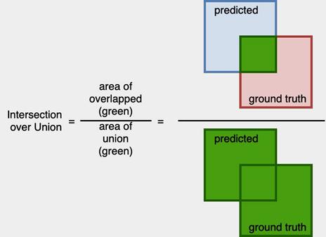
The accuracy metric we used is the Intersection over Union (IoU).
Problem Statement
There are three problems we had to solve in our project, including the generalization of the Model, and the data set labeling:
01-MANUAL
LABELING OF LARGE DATASETS:
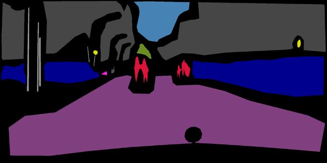
The supervised approach requires a lot of annotated data. The pixel-level labeling of large datasets [such as Cityscapes] is extremely costly due to the amount of human effort required [Manual Labeling]. Like in Figure 3.a
02-DEALING WITH DIFFERENT CONTEXTS IN SELF-DRIVING
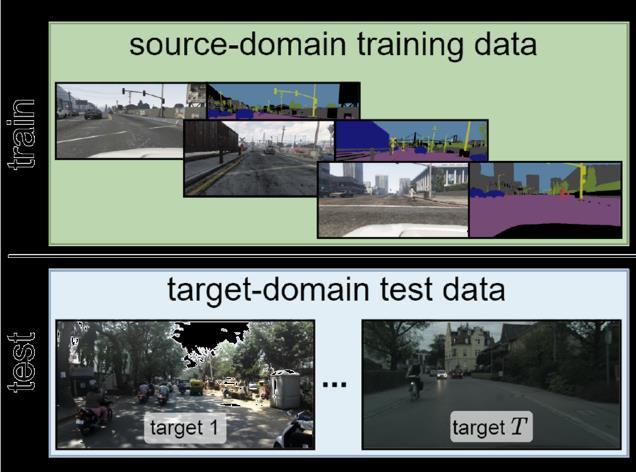
In the context of self-driving cars, the perception system is often put to test in various scenarios including different cities, weathers, or lighting conditions. There is a distribution shift under different contexts, as we see in Figure3.b, the source is from one Domain and multi-target So this will be a problem if the model is ungeneralizable.
CARS:
03-LITERATURE DEALS WITH MULTIPLE CONTEXTS AS A SINGLE-TARGET:
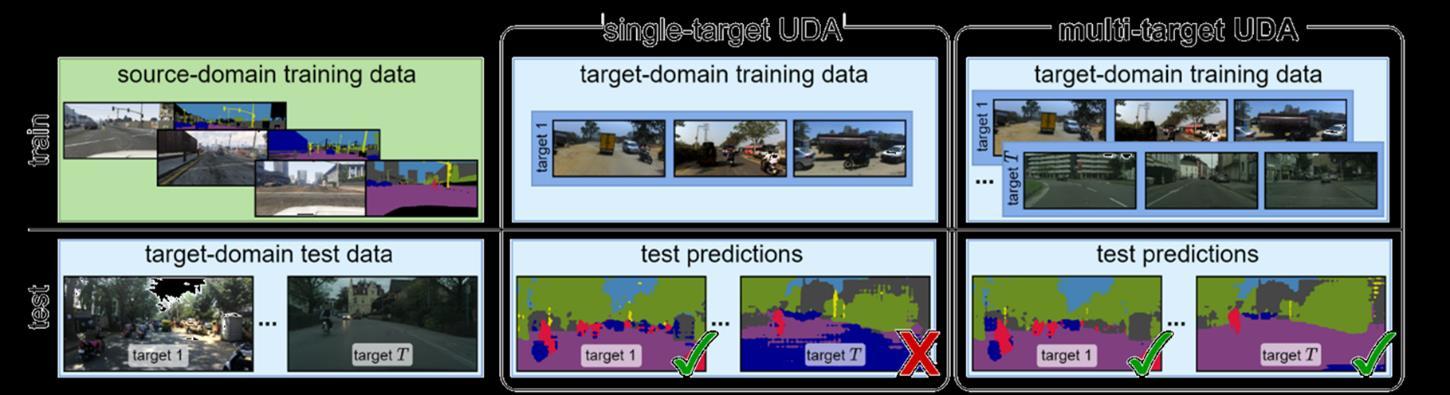
Most previous works address the single-target setting whose goal is to adapt from source to a particular target domain of interest. To deal with multiple test distributions, one can adopt single-target techniques by either:
▪ Training multiple models for all target domains and adaptively activating one at test time → This Strategy raises storage issues for embedded platforms.
▪ Merging all target data and treating them as being drawn from a single target distribution. → This Strategy overlooks distribution shifts across different target domains.
Fig3.a: Coarsely segmented image.
Fig3.b: Different contexts/target domains
Our Objectives
In this work, we address the task of unsupervised domain adaptation (UDA) for semantic segmentation in presence of multiple target domains: our objective is to train a single model that can handle all these domains at test time. Such a multi-target adaptation is crucial for a variety of scenarios that real-world autonomous systems must handle. It is a challenging setup since one face not only the domain gap between the labeled source set and the unlabeled target set but also the distribution shifts existing within the latter among the different target domains
01- UNSUPERVISED DOMAIN ADAPTATION [UDA]:
Train a Single Model that can handle MULTIPLE domains at test time. Train a model on an unlabeled target domain (real-world urban scenes) [Mapillary + Cityscapes], by leveraging a fully labeled source domain (e.g. Synthetic data).
02- IMAGE SEGMENTATION:
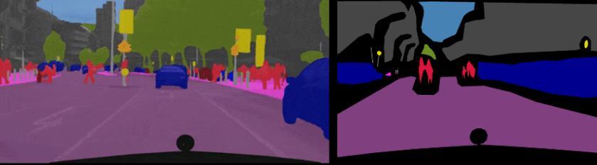
Semantic Segmentation: classifies each pixel in the image and represents different categories to color. We propose generating labels for the unlabeled large datasets to be used in future supervised learning tasks.
03- SELF-DRIVING CAR IN CARLA SIMULATOR:
Train a Self-Driving Car agent by segmenting the RGB Camera image streaming from an urban scene in the CARLA simulator to simulate the autonomous behavior of the car inside the game utilizing the Reinforcement learning technique Deep Q-Network [DQN].
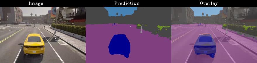
Fig4.a: Dealing with the problem using different UDA methods.
Fig4.b: Image Segmentation
Fig4.c: DQN_car agent inside Carla simulator
Datasets
We build our experiments on Three Urban driving datasets, one being synthetic, and the others being recorded in various geographic locations. We standardize the label set with 7 super classes, common to all datasets: → [Flat, construction, object, nature, sky, human, and vehicle].
01- GTA5 (GRAND THEFT AUTO 5) DATASET:
is a dataset of 24966 synthetic images sized 52 GB and 5000 synthetic images, sized 10 GB, the images have been rendered using the open-world video game Grand Theft Auto 5 and are all from the car perspective in the streets. The dataset is synthetic images with pixel-level semantic annotation with 19 classes that are compatible with the ones of the Cityscapes dataset in American-style virtual cities.
02- CITYSCAPES DATASET:
contains labeled urban scenes from 50 cities in Europe, split in training and validation sets of 5000 annotated images with fine annotations and 20 000 annotated images with coarse annotations, with 35 classes such as humans, cars, road, sky, etc. It has a large number of dynamic objects and several seasons (spring, summer, and fall) by Varying scene layout and background.
03- MAPILLARY DATASET:
is a dataset that is 5x larger than the total amount of fine annotations for Cityscapes and contains images from 190 countries around the world, it is composed of 25,000 high-resolution images annotated in a dense and finegrained style by using polygons for delineating individual objects, with 66 object categories with additional, instance-specific labels for 37 classes. Though all contain urban scenes, the datasets have different labeling policies and semantic granularity. We standardize the label set with 7 super classes, common to all datasets: flat, construction, object, nature, sky, human, and vehicle.
Literature and our Old Trials
Most recent works in UDA for semantic segmentation, adopt an adversarial training strategy either at feature level or output level. Some works also include Style Transfer or Image Translation to obtain target-looking source images while keeping source annotation.
We have tried two experiments before settling to the current setup.
▪
▪
PIX2PIX Image-to-Image Translation.
PIX2PIX-HD Image-to-Image Translation.
As shown in Figure 6.a the pix2pix or image2image translation is based on GANS architecture which is composed of the Generator (G) and discriminator (D). Simply, the generator generates fake images to fool the discriminator. But the discriminator tries to discriminate the fake image by comparison with the real image to decide if the generated image is synthesized or real
GAN Architectue: [ Generator + Discriminator]
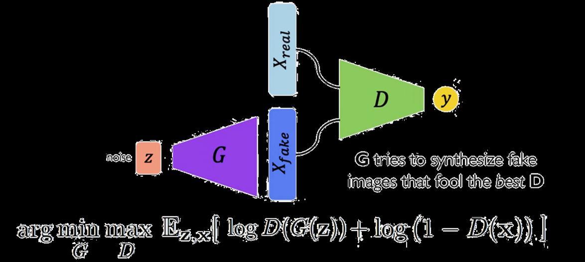
The total loss Function of generator and discriminator. Fig6.a -
Conditional GAN:
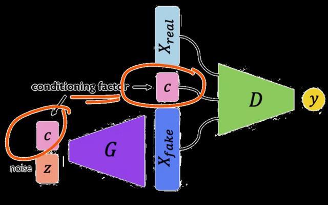
In conditional GAN is the same idea as the standard GAN except that the generator will generate the image based on a Condition. The Generator and b both receive some additional conditioning input information. This could be the class of the current image or some other property. The result of pix2pix was not that good to dig in, as we see in figure 7-a-2, so we tried also the pix2pix HD as the improvement of pix2pix, but unfortunately, the results were not satisfied because the colors are merged in together because it's based on style transfer. And you can see the results in figure 7-b-2.
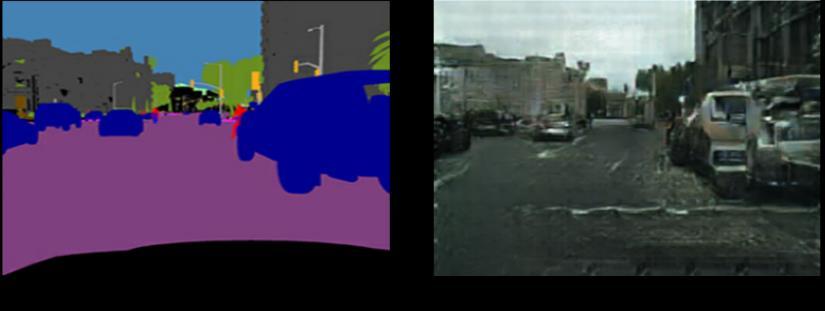
01- PIX2PIX Image-to-Image Translation:
It was not promising as shown below in this result. The syntenic image did not look to be real one however it looks it exists in the Cityscapes distribution.
02- PIX2PIX-HD:
It was not promising as well. As shown below in this result, the syntenic image did not look to be real and it seems to be worse than the Pix2Pix Also, the result is over smoothed as it is based on the CycleGAN repo.
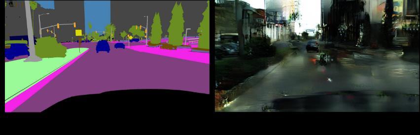
Fig7-a
Fig7-b
Methodology
we used deeplap-v2 as our model it is built upon the resnet-101 backbone initialized with ImageNet pre-trained weights, conducted with Pytorch, the deep Lab pipeline as it appears in figure 8-a
DEEP LAP V2
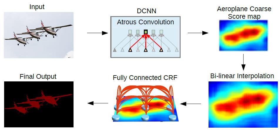
It uses ResNet-101:
▪ Atrous Convolution.
▪ Atrous Spatial Pyramid Pooling (ASPP) – [New in V2].
▪ Fully Connected Conditional Random Field (CRF).
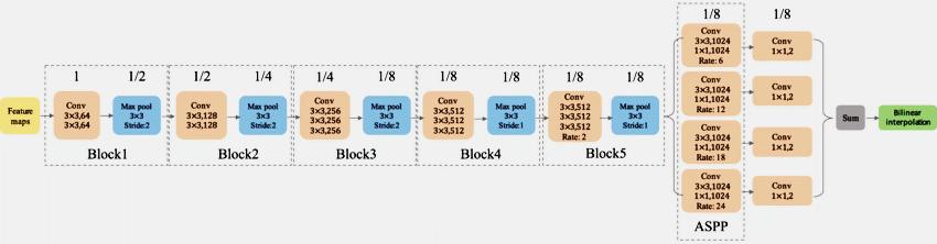
- explain the backbone of deep lab version-2 model.
Fig8-a: Deeplap V2 Pipeline
Fig8-b
01-
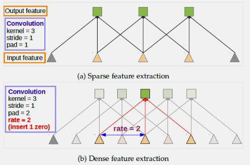
Atrous Convolution:
▪ It is also called “algorithme à trous” and “hole algorithm”.
▪ It is also called “dilated convolution”.
▪ It is commonly used in wavelet transform and right now it is applied in convolutions for deep learning.
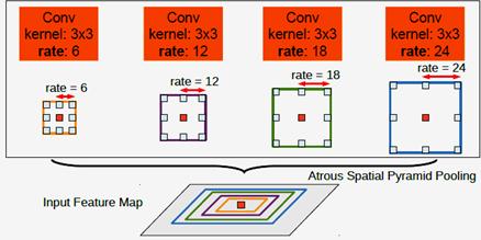
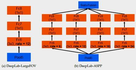
02- Atrous Spatial Pyramid Pooling (ASPP):
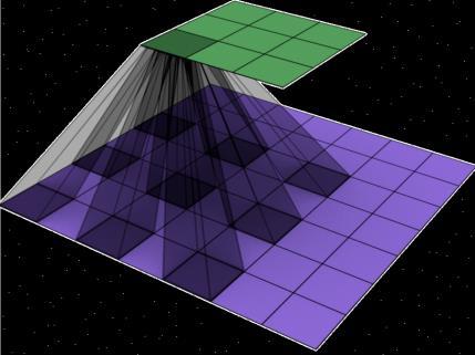
▪ ASPP is an atrous version of SPP, in which the concept has been used in SPPNet.
▪ In ASPP, parallel atrous convolution with different rates are applied in the input feature map, and fuse together.
▪ As objects of the same class can have different scales in the image, → ASPP helps to account for different object scales which can improve the accuracy.
03- Fully Connected Conditional Random Field (CRF):
▪ Fully Connected CRF is applied at the network output after bilinear interpolation.
▪ It is the weighted sum of two kernels:
▪ The first kernel depends on pixel value difference and pixel position difference, which is a Bilateral filter that has the property of preserving edges.
▪ The second kernel only depends on pixel position difference, which is a Gaussian filter
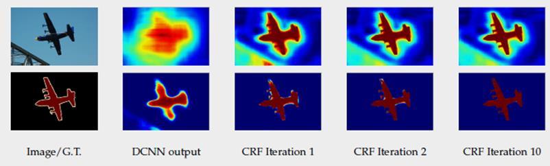
Fig9-a-1: Atros Convolution
Fig9-a-2: : Atros Convolution
Fig9-b-1: ASPP
Fig9-b-2: ASPP
Fig10-a: CRF
Adversarial Adaptation to Multiple Targets
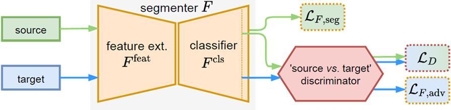
As we decided to work with two models Baseline and MTKT, Our first Model `Baseline` strategy is to merge all target datasets into a single one and then deal as a single target. Figure 11-a.
# BASELINE – AdvEnt:
▪ The Segmenter F is decoupled into a Feature Extractor [Ffeat] followed by a Pixelwise Classifier [Fcls].
▪ Handle ONLY one Source Domain and one Target Domain
▪ In Multiple Target Domains, we merge all target datasets into a single one
▪ It utilizes an existing single-source single-target UDA framework.
# Multi-Target Knowledge Transfer [MTKT] - Multiple Teachers – Single Student Approach:
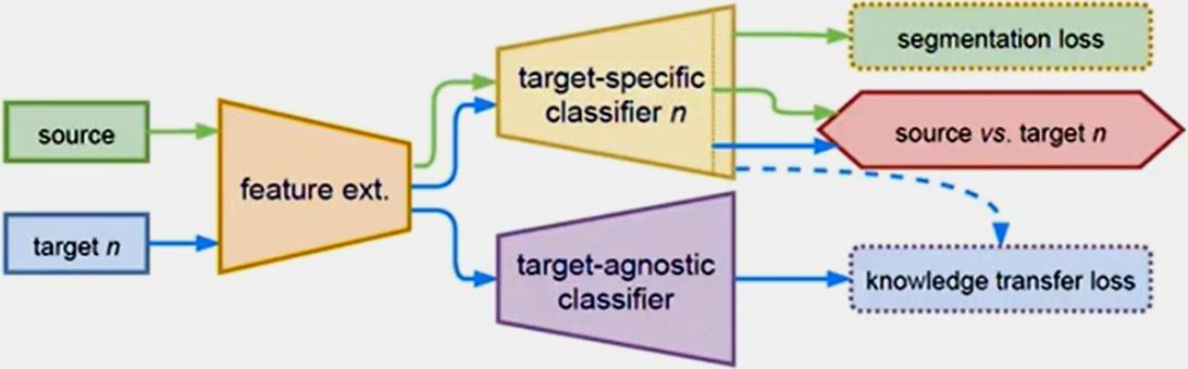
In our second model `MTKT` is a multi-target knowledge transfer, which has a target-specific teacher for each specific target that learns a target-agnostic model thanks to a multiteacher/single-student distillation mechanism. See Figure 11-a.
There are two types of classifier branches:
▪ Target-specific branches [Multiple Teachers]: → Each one handles one specific [source-target] domain shift.
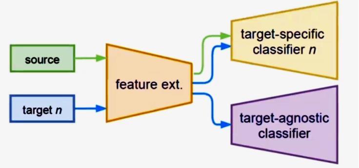
Fig11-a: Baseline Architecture
Fig11-b: Target-specific branches [Multiple Teachers]
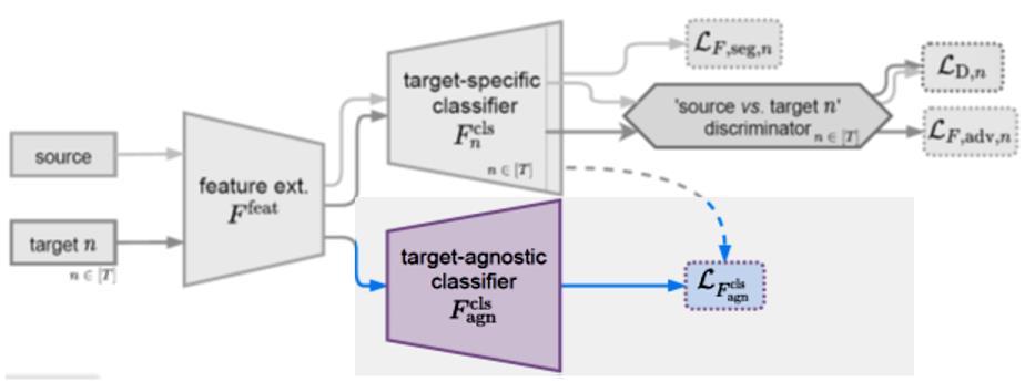
▪ Target-agnostic branch [One Student]: → It fuses all the knowledge transferred from the target-specific branches
Target-agnostic branch [One Student]
LOSS FUNCTIONS
#1 Adversarial Discriminator Loss:
▪ The Discriminator [D] is a fully-convolutional binary classifier with parameters (φ).
▪ It classifies the Segmenter’s output (Qx) into either: class 1 (source) or 0 (target)
EQN-1: Discriminator Loss Function
Targets [Cityscapes + Mapillary]
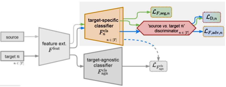
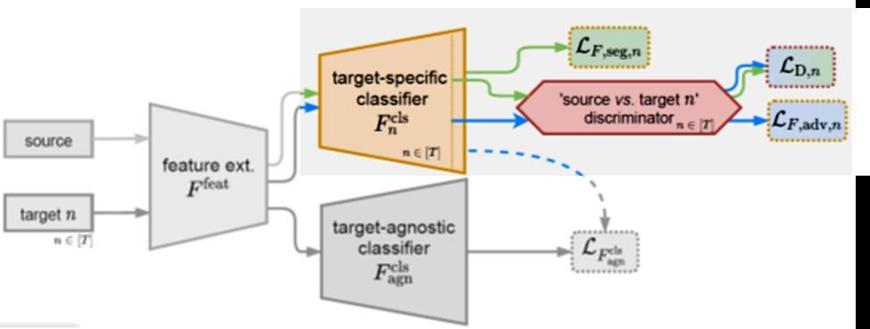
MTKT Target Specific Classifiers [Teachers], and the discriminators [one for each target]
Fig11-b:
Fig12-a:
#2 Segmentor Loss:
▪ The Segmenters [Fcls-n] is trained over its parameters (θ) NOT Only to minimize the supervised segmentation loss LF, seg on source-domain data.
▪ But also, to fool the discriminator D via minimizing an adversarial loss LF, adv.
▪ The weight [λ adv] balancing the two terms.
▪ During training, one alternately minimizes the two losses LD and LF.

EQN-2: Segmentor Loss Function
Fig13 2 Target-specific classifiers + 2 Discriminators.
#3 Knowledge Transfer Loss:
▪ The Agnostic classifier [Fcls-agn] is trained over its parameters to minimize over the segmenter’s parameters (including feature extractors).
▪ The [Student] fuses all the knowledge transferred from the T-target-specific classifiers [Teachers] via minimizing the Kullback-Leibler divergence between teachers’ and student’s predictions on target domains.

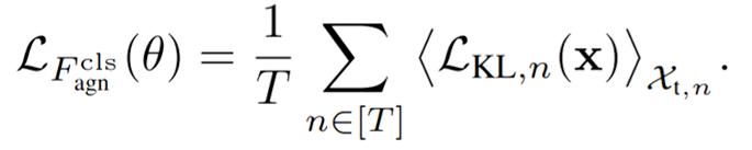
EQN3-a: Kullback Libler Divergence between the student’s prediction and teacher’s predictions
EQN3-b: Knowledge Transfer Loss using the Kullback Libler Divergence between the student and each teacher predictions
Fig14: MTKT Target Agnostic Classifier [Student]
Implementation Details
We preferred using PyTorch as our Framework, as we mentioned before we used the pretrained Deep Lab Model version 2,
The below table shows the implementation details that we used in our experiment:
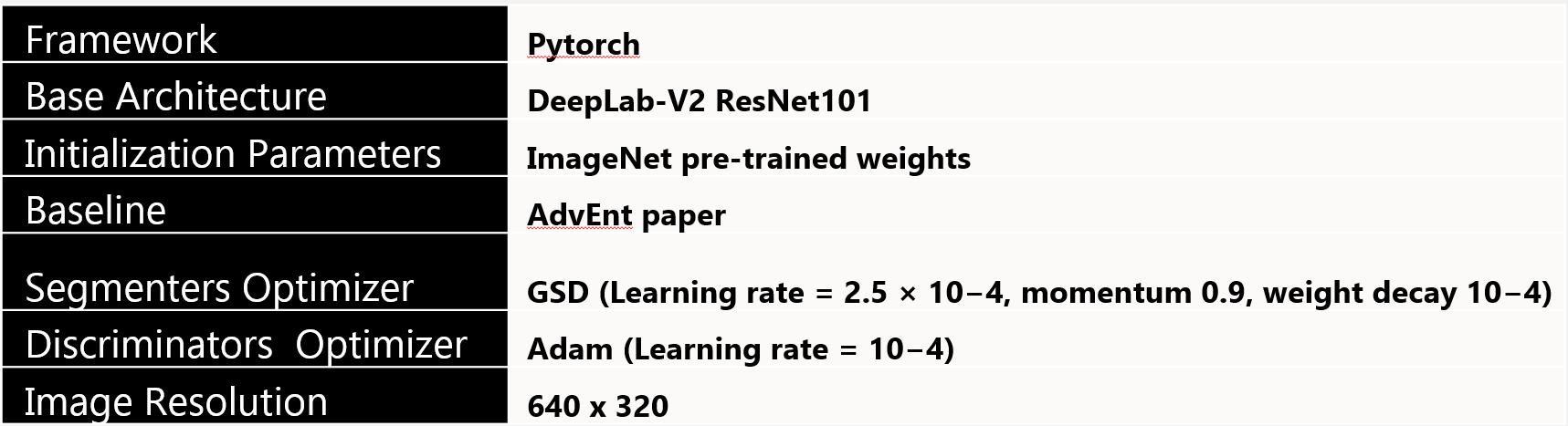
The important point here is the target-specific branches, which is the teacher as figure 13 explains. We try to learn the feature with 20000 iterations
▪ In MTKT, we “warm-up”the Target-specific branches for 20,000 iterations before training the Target-agnostic branch.
▪ The warm-up step avoids the distillation of noisy target predictions in the early phase, which helps stabilize Target-agnostic training.
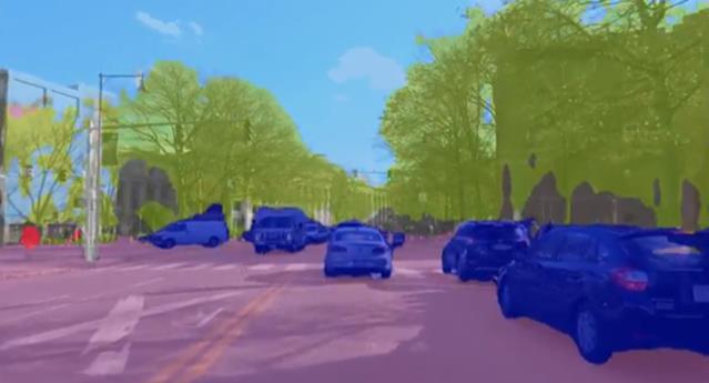
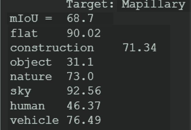
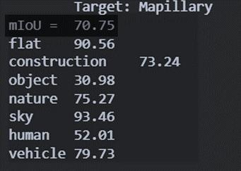
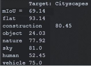
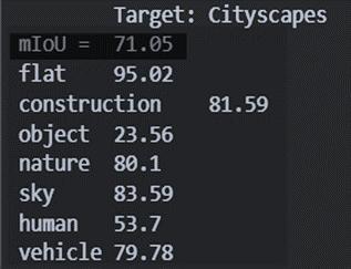
In all tested scenarios, the MTKT approach consistently outperforms baselines
Evaluation Metrics - Intersection over Union [ IoU ]
As shown in figure 16-a-2, the IoU is the intersection of predicted and Ground Truth over the union between them.
Mapillary
BASELINE
MTKT
Cityscapes
IoU Score
Features that we care more about
Fig16-a-1: Result of the segmentation model.
Fig16-b-1: Summary Statistics on the Mapillary Datasets
Fig16-b-2: Summary Statistics on the Cityscapes Datasets
Fig16-a-2: Intersection over Union [IoU]
Predict Images with Coarse Segmentation in Cityscapes
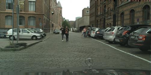
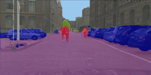
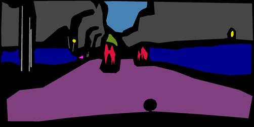
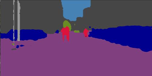
The RGB image in fig 17-a-1 is one of the 20000 images from the Cityscapes dataset. The ground truth of the RGB image is coarsely segmented, so as our model predicted the fine annotated segmentation that appears in figure 17-a-2. We propose that to use it as ground truth instead of coarse segmentation GT.
MTKT Outperforms the Baseline clearly in some examples:
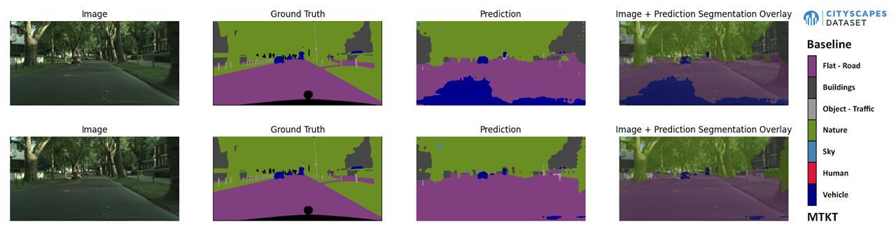
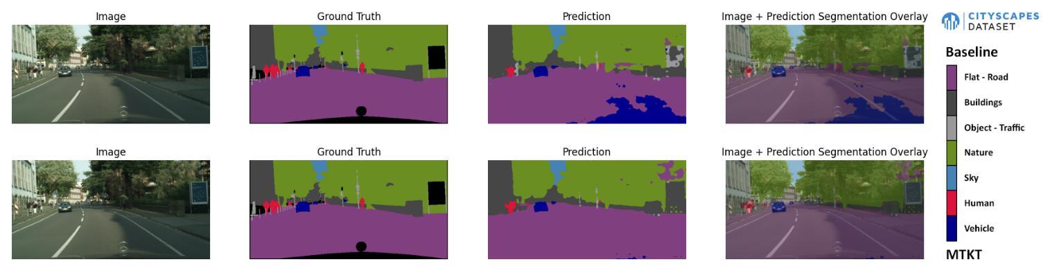
Fig17-a-2
Fig17-a-1 Coarse Segmentation Our Segmentation
Fig17-b-1: Comparison between Baseline and MTKT on Cityscapes test dataset.
Fig17-b-2: Comparison between Baseline and MTKT on Mapillary test dataset.
Comparison between BASELINE vs MTKT:
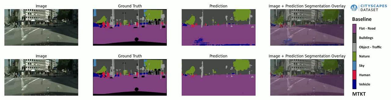
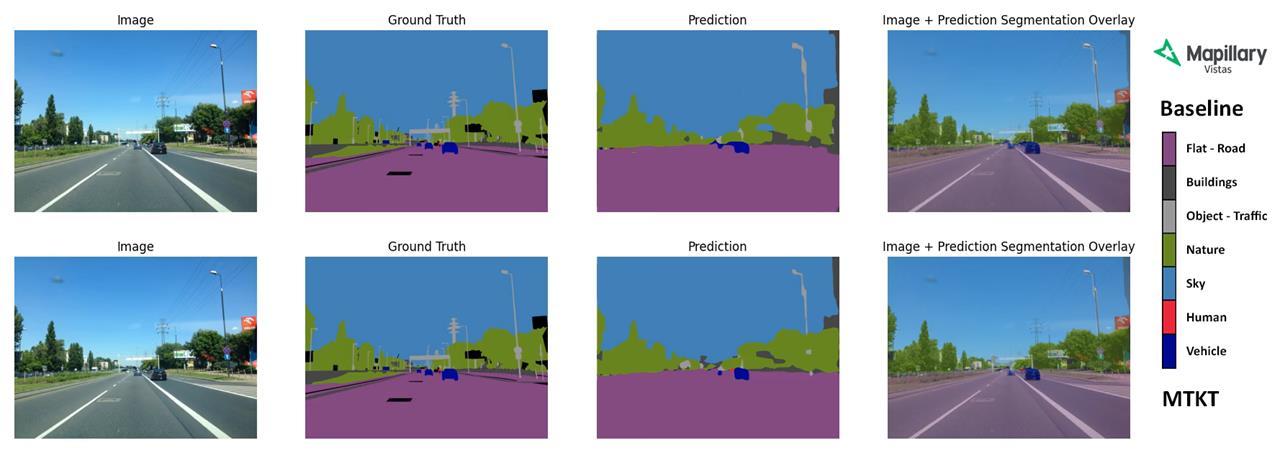
We can notice the difference between the two models, the MTKT performs better than the baseline Our Segmentation of a Video example from Cityscapes:
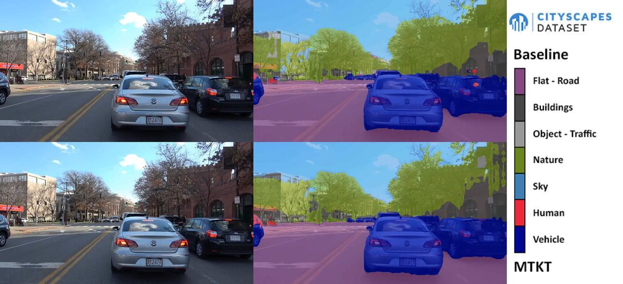
Fig18-a Comparison between Baseline and MTKT on Cityscapes test dataset.
Fig19 Video Segmentation using Baseline and MTKT
Fig18-b Comparison between Baseline and MTKT on Mapillary test dataset.
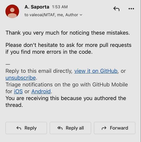
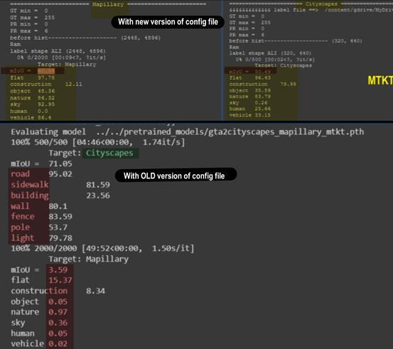
Our Contribution and Accepted Pull-Request on Valeo France Repo:
There was a bug in the configuration file in the code of the main value branch repo, and we pulled a request to merge on the main branch for Value France.
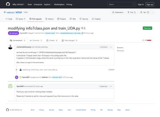
The Difference between our IoU, and their IoU
Deployment
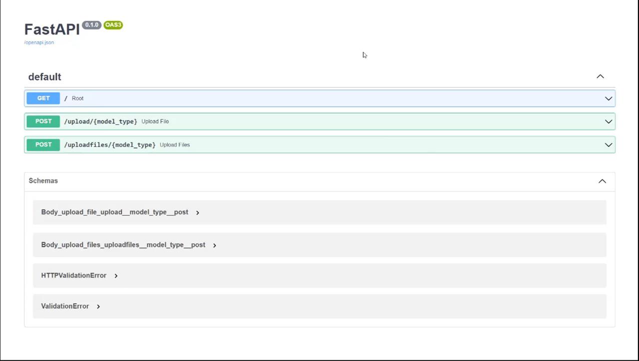
This project is a Web API for Urban Scene Segmentation for Autonomous Car, using two models `Baseline` and `MTKT`, that can handle unsupervised domain adaptation (UDA) problem for multi-target datasets.
In FastAPI documentation we propose our two functions that we use to segment labeled images and unlabeled images, and we make a web client that propose the Two functions also



Reinforcement learning in our project
Deep Reinforcement Learning – DQN in Carla:
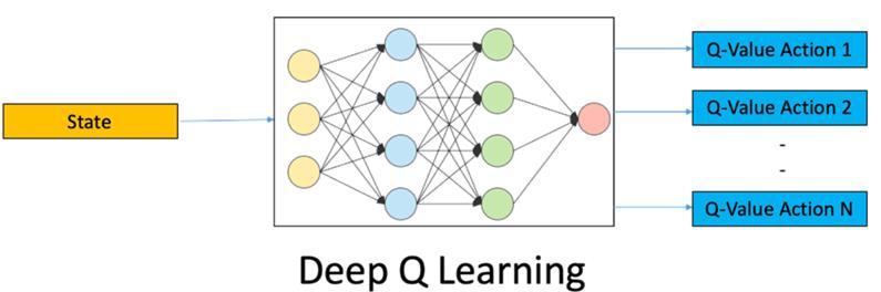
▪ In deep Q-learning, we use a Neural Network to approximate the Q-value function, which is called a Deep Q Network [DQN].
▪ This function maps a state [Input] to the Q-values of all the actions that can be taken from that state [Output].
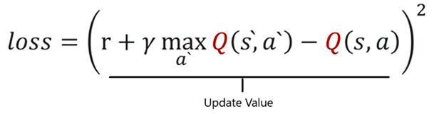
DQN Algorithm:
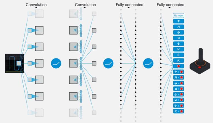
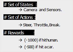
Fig22-a: Deep Q-Learning
Fig23-a: DQN Architecture
Fig23-b: Sample of the Set of states, actions, and rewards
DQN Algorithm and Architecture Components
1. Feed the DQN Agent with the preprocessed segmented urban scene image (state s) and it returns the Q-values of all possible actions in the state [different values for throttle, steer].
2. Select an Action using the Epsilon-Greedy Policy
a. With the probability epsilon, we select a random action a.
b. With the probability 1-epsilon, we select an action that has a maximum Q-value, such as a = argmax(Q(s,a,w)).
3. Perform this Action in a state s and move to a new state s’ to receive a reward.
a. This state s’ is the next image.
b. We store this transition in our Replay Buffer as <s,a,s’>

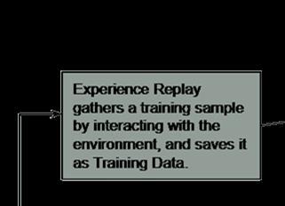

Fig23-c: Replay Memory in the DQN
4. Next, sample some Random Batches of transitions from the Replay Buffer.
5. Calculate the Loss → which is just the squared difference between target-Q and predicted-Q.
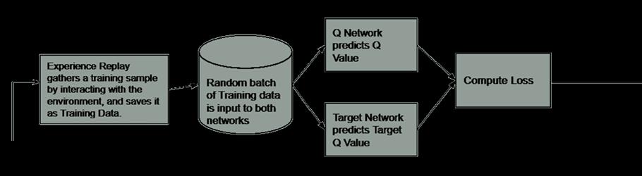

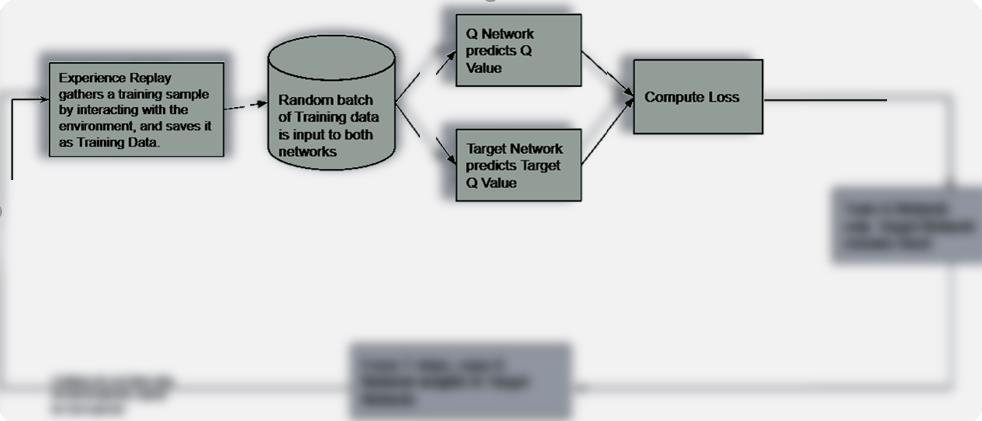
Fig24-a: Q-Network and Target Network
Fig24-b: Update the DQN Network’s parameters
7. After every C iteration, copy our actual network weights to the Target network weights.
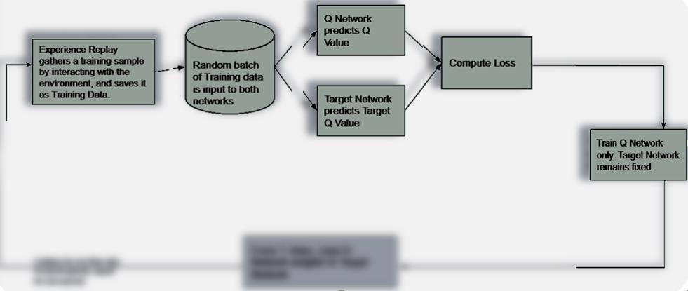
8. Repeat these steps for M number of episodes.
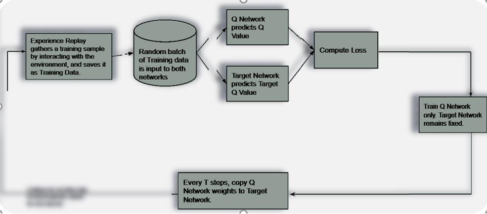
Fig25-a: Update the Target Network using the DQN Network’s parameters
Fig25-b: Repeat the previous steps over certain number of epochs
DQN Architecture Components
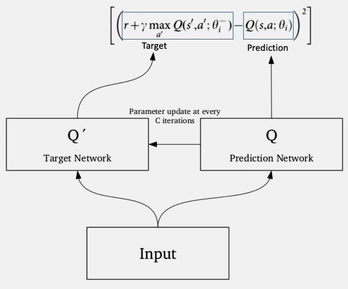
#1 Target Network:
▪ The Target network is identical to the Q network.
▪ The Target network takes the Next State from each data sample and predicts the best Q-value out of all actions that can be taken from that state which is the Target Q-Value
▪ The Target network is NOT-trained and remains fixed, so no Loss is computed.
▪ After every C iteration, the Target Network is updated by the Agent Network weights.
#2 Experience Replay:
▪ Experience Replay interacts with the Environment to generate data to train the QNetwork.
▪ It selects an ε-greedy action from the current state, executes it in the environment, and gets back a reward and the next state.
▪ Save Transitions ( St, At, Rt+1, St+1) into buffer and sample batch B.
▪ Use batch B to train the agent
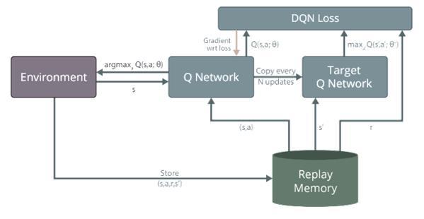
Fig26: DQN Network Target Network
Fig27: Experience Replay
#3 Epsilon Greedy Policy:
▪ Deep Q-Network starts with arbitrary Q-value estimates and explores the using the → ε-greedy policy.
▪ With the probability epsilon, we select a Random Action a.
▪ With the probability 1-epsilon, we select an action that has a maximum Q-value such as: → a = argmax(Q(s,a,w))
▪ It balances the Exploration/Exploitation.
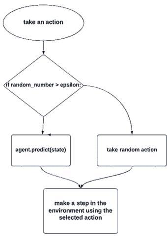
Fig28: Epsilon Greedy Policy
Our CARLA Simulator
CARLA provides open digital assets (urban layouts, buildings, vehicles) that were created for this purpose and can be used freely. The simulation platform supports flexible specification of sensor suites, environmental conditions, full control of all static and dynamic actors, maps generation, and much more.
- This project shows how to train a Self-Driving Car agent by segmenting the RGB Camera image streaming from an urban scene in the CARLA simulator to simulate the autonomous behavior of the car inside the game, utilizing the Reinforcement Learning technique Deep QNetwork [DQN].
DQN Agent inside CARLA Simulator:
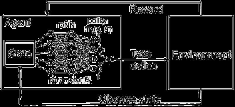
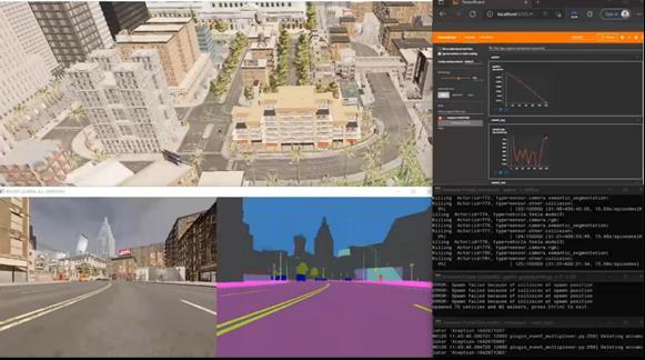
Fig29-a: Full Architecture of the DQN using Carla Simulator
Fig29-b: The training process of the DQN Agent inside Carla and Visualizing the rewards on the top right
Future Works
▪ We recommend trying the same framework on other domains [real urban datasets].
▪ Try with another base model such as Deep lap V3, ProDA ,
▪ Or with another faster base model architecture, to be replaced the Deep lab version-2 even the model is less accuracy but will be Faster, and to be tested on the both models: baseline, and MTKT.
▪ Impalement Different Deep Reinforcement learning algorithms such as the Actor-Critic and Game-GAN, and utilize the parallel processing.
References
[1] S.Kim, J.Philion, A.Torralba , S.Fidler, “DriveGAN: Towards a Controllable High-Quality Neural Simulation,” Computer Vision and Pattern Recognition ; Robotics, Apr 2021, Available: arXivLabs, https://arxiv.org/abs/2104.15060 . [Accessed November 2021].
[2]P.Mody, “List of Semantic Segmentation Models for Autonomous Vehicles,” playment.io,March. 6, 2018.[Online].Available:https://www.playment.io/blog/semantic-segmentation-models-autonomous-vehicles . [Accessed November 2021].
[3]C.Trivedi, “How to create realistic Grand Theft Auto 5 graphics with Deep Learning,” freeCodeCamp,August.1,2018.[Online].Available:https://www.freecodecamp.org/news/how-to-create-realisticgrand-theft-auto-5-graphics-with-deep-learning-cc092c4a69f0/ [Accessed November 2021].
[4] D.Mwiti, K.(Yi) Li, “Image Segmentation in 2021: Architectures, Losses, Datasets, and Frameworks, ”neptune.ai,Dec.21,2021.[Online].Available:https://neptune.ai/blog/image-segmentation.[Accessed November 2021].
[5]T.Wang, M.Liu, J.Zhu, A.Tao, J.Kautz, B.Catanzaro, “High-Resolution Image Synthesis and Semantic Manipulation with Conditional GANs,” Computer Vision and Pattern Recognition; Graphics; Machine Learning, Nov 30, 2017 , Available: arXivLabs,https://arxiv.org/abs/1711.11585. [Accessed November 2021].
[6] J.Brownlee, “How to Develop a Conditional GAN (cGAN) From Scratch, ”machinelearningmastery com,September 1, 2020.[Online].Available:https://machinelearningmastery.com/how-to-develop-a-conditional-generativeadversarial-network-from-scratch/.[Accessed October 2021].
[7]G.Giacaglia,“HowTransformersWork, ”towardsdatascience.com,Mar 11, 2019· .[Online].Available:https://towardsdatascience.com/transformers-141e32e69591.[Accessed November 2021].
[8]M.Phi, “Illustrated Guide to LSTM and GRU’s: A step by step explanation, ”towardsdatascience.com, Sep 24, 2018. [Online]. Available:https://towardsdatascience.com/illustrated-guide-to-lstms-and-gru-s-a-step-bystep-explanation-44e9eb85bf21.[Accessed October 2021].
[9]V.Perez, “Transformers in Computer Vision: Farewell Convolutions!, ”towardsdatascience.com, November 23, 2020. [Online]. Available:https://towardsdatascience.com/transformers-in-computer-vision-farewellconvolutions-f083da6ef8ab. [Accessed November 2021].
[10]A.Saporta, T.Hung, M.Cord, P.Perez, “Multi-Target Adversarial Frameworks for Domain Adaptation in Semantic Segmentation,” Computer Vision and Pattern Recognition ; Robotics, Apr 2021, Available: Valeo.ai, https://arxiv.org/pdf/2108.06962.pdf . [Accessed December 2021].
[11]S.Richter, V.Vineet, S.Roth, V.Koltun, “Playing for Data: Ground Truth from Computer Games,” Aug.7,2016,Available:paperswithcode.com,https://paperswithcode.com/paper/playing-for-data-ground-truthfrom-computer [Accessed December 2021].
[12]T.Wang, M.Liu, J.Zhu, A.Tao, J.Kautz, B.Catanzaro, “Image-to-Image Translation with Conditional Adversarial Networks,” Nov 26, 2018, Available:paperswithcode.com,https://paperswithcode.com/paper/imageto-image-translation-with-conditional. [Accessed December 2021].
[13] J.Zhu, T.Park, P.Isola, A.Efros, “Unpaired Image-to-Image Translation using Cycle-Consistent Adversarial Networks,” Aug 24, 2020, Available:paperswithcode.com,https://paperswithcode.com/paper/unpaired-image-toimage-translation-using. [Accessed November2021].
[13]M.Uriˇcˇa´rˇ , P.Kr´ıˇzek ˇ , D.Hurych , I.Sobh, S.Yogamani, P.Denny, “Yes, we GAN: Applying Adversarial Techniques for Autonomous Driving,” March 15, 2019, Available: arXivLabs, https://arxiv.org/abs/1902.03442 [Accessed November2021].
[14]H.Huang , E.Tseng, P.Chiang , C.Lin, “Urban Scene Segmentation for Autonomous Vehicles,” March 15, 2019, Available: noiselab.ucsd.edu, http://noiselab.ucsd.edu/ECE228_2018/Reports/Report8.pdf. [Accessed November2021].
[15]N.Gählert, N.Jourdan, M.Cordts, U.Franke, J.Denzler, “Cityscapes 3D: Dataset and Benchmark for 9 DoF Vehicle Detection,” June 14, 2020, Available:Mercedes-Benz AG, arXivLabs, https://arxiv.org/abs/2006.07864 [Accessed November2021].
[16]A.Garcia, S.Escolano, S.Oprea, V.Martinez, J.Rodriguez, “A Review on Deep Learning TechniquesApplied Semantic Segmentation,” April 22, 2017, Available: arXivLabs, https://arxiv.org/abs/1704.06857 [Accessed November2021].
[17]A.Vaswani, N.Shazeer, N.Parmar, J.Uszkoreit, L.Jones, A.Gomez, L.Kaiser, I.Polosukhin, “Attention Is All You Need,” December 6, 2017, Available: arXivLabs, https://arxiv.org/abs/1706.03762. [Accessed November2021].
[18]C.Finn, P.Christiano, P.Abbeel, S.Levine, “A Connection between Generative Adversarial Networks, Inverse Reinforcement Learning, and Energy-Based Models,” November 25, 2018, Available: arXivLabs, https://arxiv.org/abs/1706.03762. [Accessed October 2021].