Issuu

Applied Numerical Methods with MATLAB for Engineers and Scientists 2nd Edition

Steven Chapra 007313290X

9780073132907

Download solution manual at: https://testbankpack.com/p/solution-manual-for-applied-numerical-methods-withmatlab-for-engineers-and-scientists-2nd-edition-steven-chapra-007313290x9780073132907/

CHAPTER 14

14.1 The data can be tabulated and the sums computed as

which can be solved for the coefficients yielding the following best-fit polynomial F

Here is the resulting fit:

PROPRIETARY MATERIAL © The McGraw-Hill Companies, Inc. All rights reserved. No part of this Manual may be displayed, reproduced or distributed in any form or by any means, without the prior written permission of the publisher, or used beyond the limited distribution to teachersand educatorspermitted by McGraw-Hill for their individual course preparation. If you are a student using this Manual, you are using it without permission.

⎤ 0

i x y x 2 x 3 x 4 xy x 2 y 1 10 25 100 1000 10000 250 2500 2 20 70 400 8000 160000 1400 28000 3 30 380 900 27000 810000 11400 342000 4 40 550 1600 64000 2560000 22000 880000 5 50 610 2500 125000 6250000 30500 1525000 6 60 1220 3600 216000 12960000 73200 4392000 7 70 830 4900 343000 24010000 58100 4067000 8 80 1450 6400 512000 40960000 116000 9280000 Σ 360 5135 20400 1296000 87720000 312850 20516500

⎡ 8 360 20400 ⎧a ⎫ ⎪ ⎪ 5135 ⎢ 360 20400 1296000 ⎥⎨a1 ⎬=⎨ 312850 ⎬ ⎢ ⎣20400 1296000 87720000⎥ ⎦ a2 20516500⎪ ⎭

Normal equations:

12202

= 178 4821 +16

v + 0 037202v

2000 1500 1000

The predicted values can be used to determinedthe sum of the squares. Note that the mean of the y values is 641.875.

i x y ypred (y y)2 (y ypred)2 1 10 25 -13.5417 380535 1485 2 20 70 158.8393 327041 7892 3 30 380 338.6607 68579 1709 500 0 -500 0 20 40 60 80 100

The coefficient of determination can be computed as r 2 = 1808297 213793 =0.88177

1808297

The model fits the trend of the data nicely, but it has the deficiency that it yields physically unrealistic negative forces at low velocities.

14.2 The sum of the squares of the residuals for this case can be written as

The partial derivatives of this function with respect to the unknown parameters can be determined as

Setting the derivative equal to zero and evaluating the summations gives

i i i i i i i i i i i i 4 40 550 525.9226 8441 580 5 50 610 720.625 1016 12238 6 60 1220 922.7679 334229 88347 7 70 830 1132.351 35391 91416 8 80 1450 1349.375 653066 10125 Σ 1808297 213793

n 2 2 S r =∑(yi − a1xi − a2 xi ) i=1

∂S r = 2∑[(y a x a x 2 )x ] ∂a1 i 1 i 2 i i ∂S r = 2∑[(y a x a x 2 )x 2 ] ∂a2 i 1 i 2 i i

( x 2 )a +( x 3 )a = x y ∑ i 1 ∑ i 2 ∑ i i ( x 3 )a +( x 4 )a = x 2 y ∑ i 1 ∑ i 2 ∑ i i which can be

∑x y ∑x 4 ∑x 2 y ∑x 3 a = 1 ∑ x 2 ∑ x 4 (∑ x 3 )2 i i i ∑x 2 ∑x 2 y ∑x y ∑x 3 a = 2 ∑ x 2 ∑ x 4 (∑ x 3 )2 i i i

solved for

The model can be tested for the data from Table 12.1.

Therefore, the best-fit model is

The fit, along with the original data can be plotted as

14.3 The data can be tabulated and the sums computed as

x y x 2 x 3 x 4 xy x 2 y 10 25 100 1000 10000 250 2500 20 70 400 8000 160000 1400 28000 30 380 900 27000 810000 11400 342000 40 550 1600 64000 2560000 22000 880000 50 610 2500 125000 6250000 30500 1525000 60 1220 3600 216000 12960000 73200 4392000 70 830 4900 343000 24010000 58100 4067000 80 1450 6400 512000 40960000 116000 9280000 Σ 20400 1296000 87720000 312850 20516500 a = 312850(87720000) 20516500(1296000) 1 20400(87720000) (1296000)2 =7.771024 a = 20400(20516500) 312850(1296000) 2 20400(87720000) (1296000) =0.119075

y =7.771024

0.119075x 2

x +

2500 2000 1500 1000 500 0 0 20 40 60 80 100

i x y x 2 x 3 x 4 x 5 x 6 xy x 2 y x 3 y 1 3 1.6 9 27 81 243 729 4.8 14.4 43.2 2 4 3.6 16 64 256 1024 4096 14.4 57.6 230.4 3 5 4.4 25 125 625 3125 15625 22 110 550 4 7 3.4 49 343 2401 16807 117649 23.8 166.6 1166.2 5 8 2.2 64 512 4096 32768 262144 17.6 140.8 1126.4 6 9 2.8 81 729 6561 59049 531441 25.2 226.8 2041.2

solved for the coefficients yielding the following best-fit

The predicted values can be used to determined the sum of the squares. Note that the mean of the y values is 3.3.

i x y ypred (y y)2 (y ypred)2 1 3 1.6 1.83213 2.8900 0.0539 2 4 3.6 3.41452 0.0900 0.0344 3 5 4.4 4.03471 1.2100 0.1334 4 7 3.4 3.50875 0.0100 0.0118 5 8 2.2 2.92271 1.2100 0.5223 6 9 2.8 2.4947 0.2500 0.0932 7 11 3.8 3.23302 0.2500 0.3215 8 12 4.6 4.95946 1.6900 0.1292 Σ 7.6000 1.2997 1 7 11 3.8 121 1331 14641 161051 1771561 41.8 459.8 5057.8 8 12 4.6 144 1728 20736 248832 2985984 55.2 662.4 7948.8 Σ 59 26.4 509 4859 49397 522899 5689229 204.8 1838.4 18164 Normal equations: ⎡ 8 59 509 4859 ⎤⎧a0 ⎫ ⎧ 26.4 ⎫ ⎢ 59 509 4859 49397 ⎥⎪a ⎪ ⎪ 204 8 ⎪ ⎢ 509 4859 49397 522899 ⎥⎨a ⎬=⎨1838.4⎬ ⎢4859 49397 522899 5689229⎥⎪ 2 ⎪ ⎪18164⎪ ⎣ ⎦⎩a3 ⎭ ⎩ ⎭ which can

polynomial y = 11 4887 + 7.143817x 1.04121x 2 + 0.046676x 3 Here is the resulting fit: 8 6 4 2 0 0 5 10 15 -2

The coefficient of determination can be computed as

r 2 = 7 6 1 2997 =0 829 7.6

14.4

function p = polyreg(x,y,m)

% polyreg(x,y,m):

% Polynomial regression.

% input:

% x = independent variable

% y = dependent variable

% m = order of polynomial

% output:

% p = vector of coefficients

n = length(x); if length(y)~=n, error('x and y must be same length'); end for i = 1:m+1 for j = 1:i

k = i+j-2;

s = 0; for l = 1:n

s = s + x(l)^k;

end

A(i,j) = s;

A(j,i) = s; end

s = 0; for l = 1:n

s = s + y(l)*x(l)^(i-1);

end

b(i) = s;

end

p = A\b';

Test solving Prob. 14.3:

14.5 Because the data is curved, a linear regression will undoubtedly have too much error. Therefore, as a first try, fit a parabola,

4 5 7 8 9 11 12]; >> y = [1.6 3.6 4.4 3.4 2.2 2.8 3.8 4.6]; >> polyreg(x,y,3)

-11.4887 7.1438 -1.0412 0.0467

= [3

ans =

>> format long

>> T = [0 5 10 15 20 25 30];

>> c = [14.6 12.8 11.3 10.1 9.09 8.26 7.56];

>> p = polyfit(T,c,2)

p = 0.00439523809524 -0.36335714285714 14.55190476190477

Thus, the best-fit parabola would be

c =14 55190476 0 36335714T + 0 0043952381T 2

We can use this equation to generate predictions corresponding to the data. When these values are rounded to the same number of significant digits the results are

Thus, although the plot looks good, discrepancies occur in the third significant digit.

We can, therefore, fit a third-order polynomial

>> p = polyfit(T,c,3)

p = -0.00006444444444 0.00729523809524 -0.39557936507936 14.60023809523810

Thus, the best-fit cubic would be

c =14.600238095 0.395579365T + 0.007295238T 2 0.000064444T 3

16 12 8 4 0 0 5

10 15 20 25 30

T c-data c-pred rounded 0 14.6 14.55190 14.6 5 12.8 12.84500 12.8 10 11.3 11.35786 11.4 15 10.1 10.09048 10.1 20 9.09 9.04286 9.04 25 8.26 8.21500 8.22 30 7.56 7.60690 7.61

We can use this equation to generate predictions corresponding to the data. When these values are rounded to the same number of significant digits the results are

Thus, the predictions and data agree to three significant digits.

14.6 The multiple linear regression model to evaluate is

The [Z] and y matrices can be set up using MATLAB commands in a fashion similar to Example 14.4,

>> format long

>> t = [0 5 10 15 20 25 30];

>> T = [t t t]';

>> c = [zeros(size(t)) 10*ones(size(t)) 20*ones(size(t))]';

= [ones(size(T)) T c];

The coefficients can be evaluated as

>> a = Z\y

a = 13.52214285714286

-0.20123809523810

-0.10492857142857

Thus, the best-fit multiple regression model is

o =13.52214285714286 0.20123809523810T 0.10492857142857c

We can evaluate the prediction at T = 12 and c = 15 and evaluate the percent relative error as

>> cp = a(1)+a(2)*12+a(3)*15

cp = 9.53335714285714

>> ea = abs((9.09-cp)/9.09)*100

T c-data c-pred rounded 0 14.6 14.60020 14.6 5 12.8 12.79663 12.8 10 11.3 11.30949 11.3 15 10.1 10.09044 10.1 20 9.09 9.09116 9.09 25 8.26 8.26331 8.26 30 7.56 7.55855 7.56

o = a0 + a1T + a2c

>> y = [14.6 12.8 11.3 10.1 9.09 8.26 7.56 12.9 11.3 10.1 9.03 8.17 7.46 6.85 11.4 10.3 8.96 8.08 7.35 6.73 6.2]';

= 4.87741631305987

Thus, the error is considerable. This can be seen even better by generating predictions for all the data and then generating a plot of the predictions versus the data. A one-to-one line is included to show how the predictions diverge from a perfect fit.

The cause for the discrepancy is because the dependence of oxygen concentration on the unknowns is significantly nonlinear. It should be noted that this is particularly the case for the dependency on temperature.

14.7 The multiple linear regression model to evaluate is y

The [Z] matrix can be set up as in

= 0:5:30;

Then, the coefficients can be generated by solving Eq.(14.10)

>> format long >> a = (Z'*Z)\[Z'*y]

a = 14.02714285714287

-0.33642328042328 0.00574444444444

2 3

16 12 8 4 4

12 16

= a0

a1T + a2T + a3T + a4c

>> T

>> T = [T T T]'; >> c = [0 0 0 0 0 0 0 10 10 10 10 10 10 10 20 20 20 20 20 20 20]'; >> o = [1 1 1 1 1 1 1 1 1 1 1 1 1 1 1 1 1 1 1 1 1]'; >> y = [14.6 12.8 11.3 10.1 9.09 8.26 7.56 12.9 11.3 10.1 9.03 8.17 7.46 6.85 11.4 10.3 8.96 8.08 7.35 6.73 6.2]'; >> Z = [o T T.^2 T.^3 c];

-0.00004370370370

-0.10492857142857

Thus, the least-squares fit is

y =14.027143 0.336423T + 0.00574444T 2 0.000043704T 3 0.10492857c

The model can then be used to predict values of oxygen at the same values as the data. These predictions can be plotted against the data to depict the goodness of fit.

>> yp = Z*a

>> plot(y,yp,'o')

Finally, the prediction can be made at T = 12 and c = 15,

>> a(1)+a(2)*12+a(3)*12^2+a(4)*12^3+a(5)*15

ans = 9.16781492063485

which compares favorably with the true value of 9.09 mg/L.

14.8 The multiple linear regression model to evaluate is

y = a0 + a1x1 + a2 x2

The [Z] matrix can be set up as in

>> x1 = [0 1 1 2 2 3 3 4 4]';

>> x2 = [0 1 2 1 2 1 2 1 2]';

>> y = [15.1 17.9 12.7 25.6 20.5 35.1 29.7 45.4 40.2]';

>> o = [1 1 1 1 1 1 1 1 1]';

>> Z = [o x1 x2 y];

Then, the coefficients can be generated by solving Eq.(14.10)

>> a = (Z'*Z)\[Z'*y]

a = 14.4609 9.0252

-5.7043

Thus, the least-squares fit is

y =14.4609 + 9.0252x1 5.7043x2

The model can then be used to predict values of the unknown at the same values as the data. These predictions can be used to determine the correlation coefficient and the standard error of the estimate.

>> yp = Z*a

>> SSR = sum((yp - y).^2)

SSR = 4.7397

>> SST = sum((y - mean(y)).^2)

SST = 1.0587e+003

>> r2 = (SST - SSR)/SST

r2 = 0.9955

>> r = sqrt(r2)

r = 0.9978

>> syx = sqrt(SSR/(length(y)-3))

syx = 0.8888

14.9 The multiple linear regression model to evaluate is

log Q = logα 0 +α1 log(D) +α 2 log(S)

The [Z] matrix can be set up as in

>> D = [.3 .6 .9 .3 .6 .9 .3 .6 .9]';

>> S = [.001 .001 .001 .01 .01 .01 .05 .05 .05]';

>> Q = [.04 .24 .69 .13 .82 2.38 .31 1.95 5.66]';

>> o = [1 1 1 1 1 1 1 1 1]';

>> Z = [o log10(D) log10(S)]

Then, the coefficients can be generated by solving Eq.(14.10)

>> a = (Z'*Z)\[Z'*log10(Q)]

Thus, the least-squares fit is

+ 2.6279log(D) + 0.5320log(S) Taking the inverse logarithm gives

14.10 The linear regression model to evaluate is

The unknowns can be entered and the [Z] matrix can be set up as in

Then, the coefficients can be generated by solving Eq.(14.10)

Thus, the least-squares fit is

The fit and the data can be plotted as

pp = Z*a;

plot(t,p,'o',t,pp)

= 1.5609 2.6279 0.5320

logQ

Q =101.5609 D2.6279S 0.5320 =36.3813D2.6279S 0.5320

=1.5609

p(t) = Ae 1.5t + Be 0.3t

0 05

+ Ce

>> p = [6 4.4 3.2 2.7 2 1.9 1.7 1.4 1.1]'; >> t = [0.5 1 2 3 4 5 6 7 9]'; >> Z =

exp(-0.05*t)];

[exp(-1.5*t) exp(-0.3*t)

a = 4.1375 2.8959 1.5349

p(t) = 4.1375e 1.5t + 2.8959e 0.3t +1.5349e 0.05t

a = (Z'*Z)\[Z'*p]

14.11 First, an M-file function must be created to compute the sum of the squares, function f = fSSR(a,Im,Pm) Pp = a(1)*Im/a(2).*exp(-Im/a(2)+1); f = sum((Pm-Pp).^2);

The data can then be entered as

>> I = [50 80 130 200 250 350 450 550 700]; >> P = [99 177 202 248 229 219 173 142 72];

The minimization of the function is then implemented by

>> a = fminsearch(@fSSR, [200, 200], [], I, P)

a = 238.7124 221.8239

The best-fit model is therefore P = 238.7124 I e 221.8239

I +1 221.8239

The fit along with the data can be displayed graphically.

>> Pp = a(1)*I/a(2).*exp(-I/a(2)+1);

>> plot(I,P,'o',I,Pp)

14.12 First, an M-file function must be created to compute the sum of the squares, function f = fSSR(a,xm,ym) yp = a(1)*xm.*exp(a(2)*xm); f = sum((ym-yp).^2);

The data can then be entered as

The minimization of the function is then implemented by

>> a = fminsearch(@fSSR, [1, 1], [], x, y)

a = 9.8545 -2.5217

The best-fit model is therefore y =9.8545xe 2.5217 x

The fit along with the data can be displayed graphically.

>> yp = a(1)*x.*exp(a(2)*x); >> plot(x,y,'o',x,yp)

1.3 1.5 1.7 1.9]; >> y = [0.75 1.25 1.45 1.25 0.85 0.55 0.35 0.28 0.18];

= [.1 .2 .4 .6 .9

14.13 (a) The model can be linearized by inverting it, 1 = K 1 + 1 v0 k m [S]3 k m

If this model is valid, a plot of 1/v0 versus 1/[S]3 should yield a straight line with a slope of K/km and an intercept of 1/km. The slope and intercept can be implemented in MATLAB using the Mfile function linregr (Fig. 12.12),

>> S = [.01 .05 .1 .5 1 5 10 50 100];

>> v0 = [6.078e-11

>> a = linregr(1./S.^3,1./v0)

a =

These results can then be used to compute km and K,

>> km=1/a(2)

km = 2.415474419523452e-005

>> K=km*a(1)

K = 0.39741170517893

Thus, the best-fit model is v0 = 2.415474 ×10 5[S]3 0.39741+[S]3

7.595e-9 6.063e-8 5.788e-6 1.737e-5 2.423e-5 2.43e-5 2.431e-5 2.431e-5];

1.0e+004

1.64527391375701 4.13997346408367

The fit along with the data can be displayed graphically. We will use a log-log plot because of the wide variation of the magnitudes of the values being displayed,

>> v0p = km*S.^3./(K+S.^3);

>> loglog(S,v0,'o',S,v0p)

(b) An M-file function must be created to compute the sum of the squares,

function

f = fSSR(a,Sm,v0m)

v0p = a(1)*Sm.^3./(a(2)+Sm.^3);

f = sum((v0m-v0p).^2);

The data can then be entered as >>

100];

The minimization of the function is then implemented by

>> format long

>> a = fminsearch(@fSSR, [2e-5, 1], [], S, v0)

a = 0.00002430998303

The best-fit model is therefore 2 431×10 5[S]3

v0 = 0.399763+[S]3

0.39976314533880

>> v0 = [6.078e-11 7.595e-9 6.063e-8 5.788e-6 1.737e-5 2.423e-5 2.43e-5 2.431e-5

S = [.01 .05 .1 .5 1 5 10 50

2.431e-5];

The fit along with the data can be displayed graphically. We will use a log-log plot because of the wide variation of the magnitudes of the values being displayed,

>> v0p = a(1)*S.^3./(a(2)+S.^3);

>> loglog(S,v0,'o',S,v0p)

14.14 (a) We regress y versus x to give

y = 20.6 + 0.494545x

The model and the data can be plotted as

(b) We regress log10y versus log10x to give log10 y = 0 99795 + 0 385077 log10 x

Therefore, α2 = 100.99795 = 9.952915 and β2 = 0.385077, and the power model is

y =9.952915x 0.385077

The model and the data can be plotted as

50 40 30 20 y = 0.4945x + 20.6 R2 = 0.8385 10 0 0 10 20 30 40 50 60

= 9 9529x0 3851

1 =0 019963+ 0.197464 1

Therefore, α3 = 1/0.01996322 = 50.09212 and β3 = 0.19746357(50.09212) = 9.89137, and the saturation-growth-rate model is

y =50.09212 x 9.89137+ x

The model and the data can be plotted as

(d) We employ polynomial regression to fit a parabola

y = 0.01606x 2 +1.377879x +11.76667

The model and the data can be plotted as

30 50 40 30 20 y

10 R2

0 0 10 20 30 40 50 60

= 0 9553

50 40 x y = 50.092 20 x + 9.891369 10 R2 = 0.98919 0 0 10 20 30 40 50 60

Comparison of fits: The linear fit is obviously inadequate. Although the power fit follows the general trend of the data, it is also inadequate because (1) the residuals do not appear to be randomly distributed around the best fit line and (2) it has a lower r 2 than the saturation and parabolic models.

The best fits are for the saturation-growth-rate and the parabolic models. They both have randomly distributed residuals and they have similar high coefficients of determination. The saturation model has a slightly higher r 2. Although the difference is probably not statistically significant, in the absence of additional information, we can conclude that the saturation model represents the best fit.

be displayed, reproduced or distributed in any form or

any means,

the prior written permission

the

or used

the limited distribution to teachersand educators

by McGraw-Hill for their individual

preparation.

are a student

50 40 30 20 y = -0 0161x2 + 1 3779x + 11 767 10 R2 = 0 98 0 0 10 20 30 40 50 60

without

publisher,

beyond

permitted

course

If you

using this Manual, you are using

without permission.

14.15 Linear regression gives 200 160 120 80 40 0 y = 5.8x + 60 R2 = 0.9755 0 5 10 15 20 Polynomial regression yields a best-fit parabola 200 160 120 y = 0 15067x2 + 2 78661x + 68 03571 R2 = 0.99795 80 40 0 0 5 10 15 20 Exponential model:

The linear model is inadequate since it does not capture the curving trend of the data. At face value, the parabolic and exponential models appear to be equally good. However, knowledge of bacterial growth might lead you to choose the exponential model as it is commonly used to simulate the growth of microorganism populations. Interestingly, the choice matters when the models are used for prediction. If the exponential model is used, the result is

B = 67.306e0.0503(40) = 503.3317

For the parabolic model, the prediction is

B = 0.15067t 2 + 2.78661t + 68.03571 = 420.5721

Thus, even though the models would yield very similar results within the data range, they yield dramatically different results for extrapolation outside the range.

14.16 The sum of the squares of the residuals for this case can be written as

The partial derivatives of this function with respect to the unknown parameters can be determined as

2 200 160 120 80 40 0 y = 67.306e0.0503x R2 = 0.9979 0 5 10 15 20

n 2 S r =∑(yi a1xi a2 xi ) i=1

∂S r = 2∑[(y a x a x 2 )x ] ∂a1 i 1 i 2 i i ∂S r = 2∑[(y a x a x 2 )x 2 ] ∂a2 i 1 i 2 i i

the

( x 2 )a +( x 3 )a = x y ∑ i 1 ∑ i 2 ∑ i i ( x 3 )a +( x 4 )a = x 2 y ∑ i 1 ∑ i 2 ∑ i i

Setting

derivative equal to zero and evaluating the summations gives

which can be solved for

The model can be tested for the data from Table 13.1.

a = 312850(87720000) 20516500(1296000)

1 20400(87720000) (1296000)

2 =7.771024

a = 20400(20516500) −312850(1296000)

2 20400(87720000) (1296000) =0.119075

Therefore, the best-fit model is y =7.771024x + 0.119075x 2

The fit, along with the original data can be plotted as 2500

14.17 (a) The data can be plotted as

i i i i i i i i i i i i ∑x y ∑x 4 ∑x 2 y ∑x 3 a = 1 ∑ x 2 ∑ x 4 (∑ x 3 )2 i i i ∑x 2 ∑x 2 y ∑x y ∑x 3 a = 2 ∑ x 2 ∑ x 4 (∑ x 3 )2 i i i

2000 1500 1000 500 0 0 20 40 60 80 100

regression yields

14.18 The equation can be expressed in the form of the general linear least-squares model,. PV 1= A 1 + A 1 RT 1 V V 2

>> R=82.05;T=303;

>> P=[0.985 1.108 1.363 1.631]';

>> V=[25000 22200 18000 15000]';

>> y=P.*V/R/T-1;

>> Z=[1./V 1./V.^2];

>> a=(Z'*Z)\(Z'*y)

a = -231.67 -1.0499e+005

2 2.0E-03 1.5E-03 1 0E-03 5.0E-04 0.0E+00 0 10 20 30 40 (b) Linear

3 3 μ=1.519×10 3 + 1 307×10 1.519×10 (7.5 5) =1.413×10 3 10 5

Polynomial

2.0E-03 1.5E-03 y = 5.48342E-07x2 - 4.94934E-05x + 1.76724E03 R2 = 9.98282E-01 1.0E-03 5.0E-04 0.0E+00 0 10 20 30 40 This leads to a

of μ=5.48342×10 7 (7 5)2 4.94934×10 5(7.5) +1.76724×10 3 =1.4269×10 3

interpolation yields.

(b)

prediction

Alternatively, nonlinear regression can also be used to evaluate the coefficients. First, a function can be set up to compute the sum of the squares of the residuals,

function f = fSSR1418(a,V,ym) yp=1+a(1)./V+a(2)./V.^2;

f = sum((ym-yp).^2);

Then, the fminsearch function can be employed to determine the coefficients,

>> fminsearch(@fSSR1418,[-200 1],[],V,y) ans = -231.67 -1.0499e+005

14.19 We can use general linear least squares to generate the best-fit equation. The [Z] and y matrices can be set up using MATLAB commands as

>> format long

>> x = [273.15 283.15 293.15 303.15 313.15]';

>> Kw = [1.164e-15 2.950e-15 6.846e-15 1.467e-14 2.929e-14]';

>> y=-log10(Kw);

>> Z = [(1./x) log10(x) x ones(size(x))];

The coefficients can be evaluated as

>> a=inv(Z'*Z)*(Z'*y)

Warning: Matrix is close to singular or badly scaled. Results may be inaccurate. RCOND = 6.457873e-020.

a = 1.0e+003 *

5.18067187500000

0.01342456054688

0.00000562858582

-0.03827636718750

Note the warning that the results are ill-conditioned. According to this calculation, the best-fit model is

We can check the results by using the model to make predictions at the values of the original data

>> yp=10.^-(a(1)./x+a(2)*log10(x)+a(3)*x+a(4))

yp = 1.0e-013 *

0.01161193308242

0.02943235714551

0.06828461729494

10 a

log10 K w = 5180.67

T a + 0.00562859

38.276367

+13.42456log T

T a

0.14636330575049

0.29218444886852

These results agree to about 2 or 3 significant digits with the original data.

14.20 The “Thinking” curve can be fit with a linear model whereas the “Braking” curve can be fit with a quadratic model as in the following plot.

= 5.8783E-03x2 + 9.2063E-04x - 9.5000E-02

2 = 9 9993E-01

= 0.1865x + 0.0800

= 0.9986

A prediction of the total stopping distance for a car traveling at 110 km/hr can be computed as

14.21 The angular frequency can be computed as ω0 = 2π/24= 0 261799. The various summations required for the normal equations can be set up as

The normal equations can be assembled as

100 80 60 40 20 0 y

0 20 40 60 80 100 120 140

d =0.1865(110)+0.0800 +5.8783×10 3(110)2 +9.2063×10 4 (110) 9.5000×10 2 =91.726m

t y cos(ω0t) sin(ω0t) sin(ω0t)cos(ω0t) cos 2(ω0t) sin2(ω0t) ycos(ω0t) ysin(ω0t) 0 7.6 1.00000 0.00000 0.00000 1.00000 0.00000 7.60000 0.00000 2 7.2 0.86603 0.50000 0.43301 0.75000 0.25000 6.23538 3.60000 4 7.0 0.50000 0.86603 0.43301 0.25000 0.75000 3.50000 6.06218 5 6.5 0.25882 0.96593 0.25000 0.06699 0.93301 1.68232 6.27852 7 7.5 -0.25882 0.96593 -0.25000 0.06699 0.93301 -1.94114 7.24444 9 7.2 -0.70711 0.70711 -0.50000 0.50000 0.50000 -5.09117 5.09117 12 8.9 -1.00000 0.00000 0.00000 1.00000 0.00000 -8.90000 0.00000 15 9.1 -0.70711 -0.70711 0.50000 0.50000 0.50000 -6.43467 -6.43467 20 8.9 0.50000 -0.86603 -0.43301 0.25000 0.75000 4.45000 -7.70763 22 7.9 0.86603 -0.50000 -0.43301 0.75000 0.25000 6.84160 -3.95000 24 7.0 1.00000 0.00000 0.00000 1.00000 0.00000 7.00000 0.00000 Sum→ 84.8 2.31784 1.93185 0.00000 6.13397 4.86603 14.94232 10.18401

⎧A ⎫ ⎡ 11 2.317837 1.931852⎤⎪ 0 ⎪ 84.8 ⎢ 2.3178 6 133975 0 ⎥⎨A1 ⎬=⎨14.94232⎬ ⎢ ⎣1.931852 0 4.866025⎥ ⎦ B1 ⎪ ⎩10.18401⎪ ⎭

This system can be solved for A0 = 8.02704, A1 = –0.59717, and B1 = –1.09392. Therefore, the best-fit sinusoid is

pH =8.02704 0.59717 cos(ω0t) 1.09392 sin(ω0t)

The result can also be expressed in the alternate form of Eq. 14.14 by computing the amplitude, C1 = 0.597172 +1.093922 =1.246305

and the phase shift ⎛

θ=arctan⎜ 1.09392 ⎟= 2.070488 ⎝ 0.59717⎠

Therefore, the fit can also be expressed as

pH =8 02704 +1.246305 cos(ω0t + 2.070488)

Consequently, the mean is 8.02704 and the amplitude is 1.246305. The time of the maximum can be computed as

t max = 24 2.070488× 24hr =16 09132hrs 2π

This is equal to about 16:05:29 or 4:05:29 PM. The data and the model can be plotted as

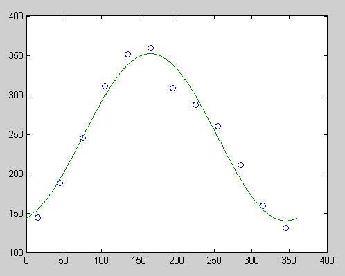
14.22 The coefficients can be determined as >>

a = 246.17 -102.36 27.405

>> tp=[0:360];

>> Rp=a(1)+a(2)*cos(w0*tp)+a(3)*sin(w0*tp);

>> plot(t,T,'o',tp,Rp)

⎞

10 9 8 7 6 0 6 12 18 24

t=[15 45 75 105 135 165 195 225 255 285 315 345]';

R=[144 188 245 311 351 359 308 287 260 211 159 131]';

Z=[ones(size(t))

cos(w0*t) sin(w0*t)]; >> a=(Z'*Z)\(Z'*R)

The value for mid-August can be computed as >> a(1)+a(2)*cos(w0*225)+a(3)*sin(w0*225) ans = 299.17

Applied numerical methods with matlab for engineers and scientists 2nd edition steven chapra solutio

Applied Numerical Methods with MATLAB for Engineers and Scientists 2nd Edition

Steven Chapra 007313290X

9780073132907

CHAPTER 14