
7.1-1.
Introduction to Operations Research 10th
Edition Fred Hillier
Full download at link:
Test Bank: https://testbankpack.com/p/test-bank-forintroduction-to-operations-research-10th-edition-hillier0073523453-9780073523453/
Solution Manual: https://testbankpack.com/p/solutionmanual-for-introduction-to-operations-research-10thedition-hillier-0073523453-9780073523453/
CHAPTER 7: LINEAR PROGRAMMING UNDER UNCERTAINTY
(a) ²% Á% Á% ³ ~ ² ° Á Á ³ , A ~
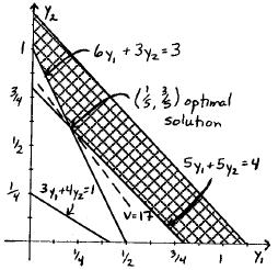
(b) minimize > ~ & b & subject to & b & ‚ & b & ‚ & b & ‚ & Á& ‚
(c) Optimal Solution: ²& Á& ³ ~ ² ° Á ° ³, > ~
7-1
(d) Since the new dual constraint & b & ‚ is violated by ²& Á& ³ ~ ² ° Á ° ³, the current solution is no longer optimal.
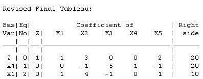
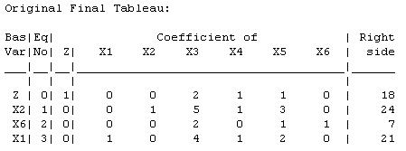
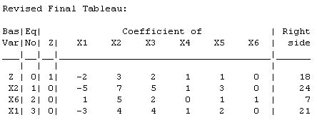
(e) New % column: c c 8 96 7 8 9
c ~
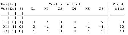
(f) The new primal variable adds a constraint to the dual, & b & ‚ , which is not satisfied by ²& Á& ³ ~ ² ° Á ° ³, so the current solution is no longer optimal.
(g) ~ c ~ c , new column: c ~ new 2 36 7 8c 96 7 8 9
7-2
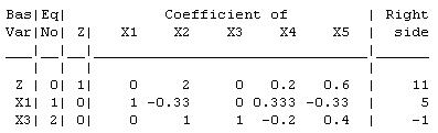
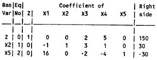
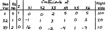
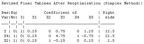
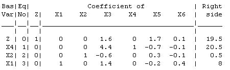
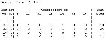
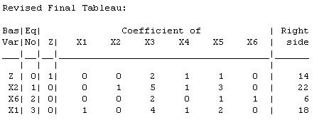
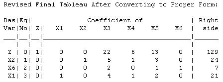
The current basic solution ²c ° Á Á Á Á ³ is infeasible and superoptimal.
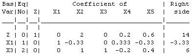
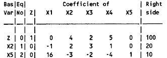
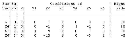
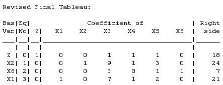
The current basic solution ² Á Á
Á Á ³ is infeasible and superoptimal.
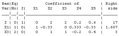
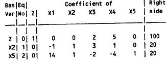
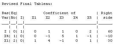
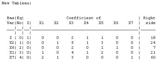
7-3 7.1-2. (a) " ~ c , " ~ ¬ "Ai ~ 2 36c 7 ~ c " i ~ c c ~ c 2 36 7 " i ~ c c ~ 2 New Tableau: 36 7
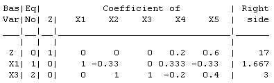
(b) " ~ , " ~ c ¬ "Ai ~ ~ c 2 36 c 7 " i ~ c ~ ° 2 36 c 7 " i ~ c ~ c 2 New Tableau: 36 c 7
c
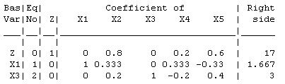
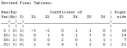
(c) " ~ ¬ "²'i c ³ ~ c
New Tableau:
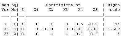
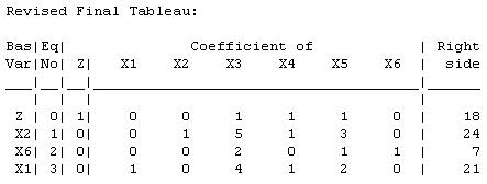
The current basic solution ² ° Á Á Á Á ³ stays optimal.
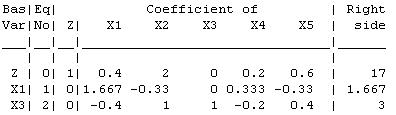
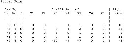
(d) " ~ c ¬ "²'i c ³ ~
New Tableau:
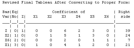
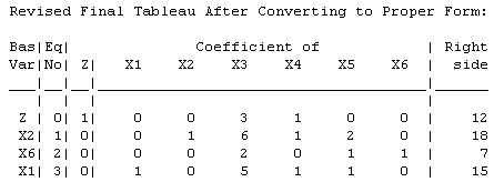
Proper Form:
The current basic solution ² ° Á Á Á Á ³ stays optimal.
(e) " ~ , " ~ c
7-4
¬
c
c 2 36c 7 " i
c
2 36c 7 " i
c ~ c 2 36c 7
"²'i
³ ~ ~
~
~
~
New Tableau:
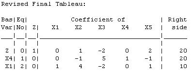
The current basic solution ²
and optimal.
Proper Form:
The current basic solution ² À Á Á À Á Á ³ is feasible and optimal.

7-5
(f) " ~ , " ~ ¬ "²'i c ³ ~ ~ 2 36 7 " i ~ c ~ 2 36 7 " i ~ c ~ c 2
° Á Á Á Á ³ is feasible
New Tableau: 36 7
New Tableau:
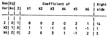
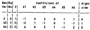
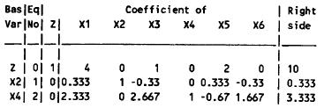
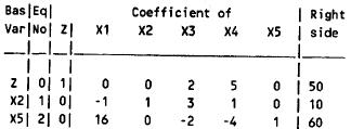
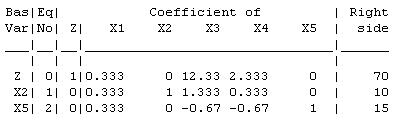
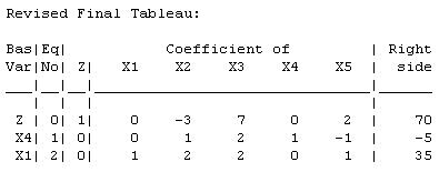
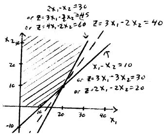
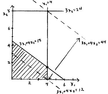
From the tableau, we see that the primal basic solution is feasible, but not optimal.
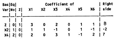
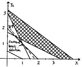
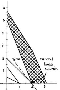
From the graph, we can see the current basic solution is feasible, but not optimal.
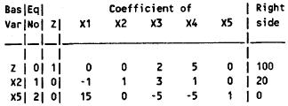
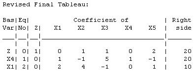
7-6 7.1-3. (a) " ~ c , " ~ ¬ "Ai ~ 6 c 7 ~ c " i ~ c 6 c 7 " i ~ c 6 c 7
~ c ~
New Tableau:
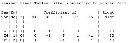
Proper Form:
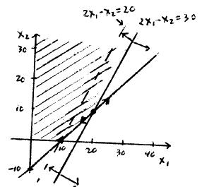
The primal basic solution is both feasible and optimal.
From the graph, we see that the current basic solution is feasible and optimal.

7-7 (b) " ~c ¬ "²'i c ³ ~ " ~ ¬ "²'i c ³ ~ c " ~ ¬ "²'i c ³ ~ c " ~ ¬ "²'i c ³ ~ c
New Tableau:
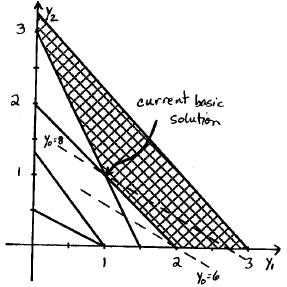
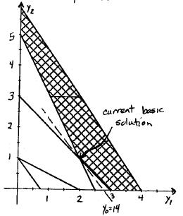
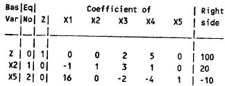
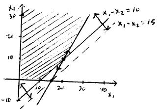
The primal basic solution is infeasible, but satisfies the optimality criterion.
From the graph, the current basic solution is infeasible and superoptimal.
7-8 " " (c) " ~ c , " ~ " ~ ¬ "²'i c ³ ~ c b c ~ c i ~ c 6 c 7 i ~ c 6 c 7 ~ c ~ 6 7
New Tableau:
Proper Form:
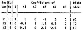
The primal basic solution is feasible and optimal.
From the graph, the current basic solution is feasible and optimal.

7-9 " (d) " ~ , " ~ " ~ ¬ "²'i c ³ ~ c b ~ c " i ~ c ~ 6 7 i ~ c 6 7 6 7 ~ c
7.2-1.
The model Ep(x) is developed to identify a long-term management plan that satisfies the legal requirements andoptimizes PALCO's operations andprofitability.The model consists of a linear program with the objective of maximizing present net worth subject to harvestflow constraints, political and environmental constraints. Detailed sensitivity analysis is performed to "determine the optimal mix of habitat types within each of individual watersheds" [p. 93]. Many instances of the LP problem are run with varying parameters. The financial benefits of this study include an increase of over $398 million in present net worth and of over $29 million in average yearly net revenues. Sustained-yield annualharvest levels have increased. The habitat mix is improved in accordance with political and environmental regulations. A more profitable long-term plan paved the way for improved short- and mid-term plans. Sensitivity analysis enabled PALCO to improve its knowledge base of the ecosystem and to adjust its plans quickly when a change in costs orinregulationsoccurs. Sinceitsdecisionsarenowjustifiedthroughasystematicapproach, PALCO is able to obtain better terms from banks. The study did not only affect PALCO and the habitat controlled by PALCO. It has also "shown that the forest product industries can coexist with wildlife and contribute to their habitats" [p. 104] and "increased quality of life for future generations" [p. 105].
7-10
(a) " ~ , " ~ ¬ "Ai ~ 6 7 ~ " i ~ 6 7 ~ " i ~ c New Tableau: 6 7 ~ c
7.2-2.
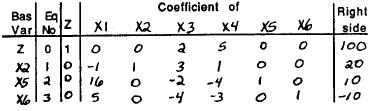
The current basic solution is infeasible and superoptimal.
The current basic solution is infeasible and superoptimal.
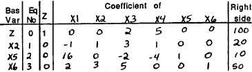
The current basic solution is feasible and optimal.
7-11 6 7 (b) " ~ , " ~ c ¬ "Ai ~ 6 c 7 ~ " i ~ 6 c 7 ~ " i ~ c 6 New Tableau: c 7 ~ c
(c) " ~ c , " ~ ¬ "Ai ~ c ~ c " i ~ 6 c 7 ~ c " i ~ c 6 c 7 ~ New Tableau:
(d) " ~ c ¬ "²'i c ³ ~
New Tableau:
The current basic solution is feasible and optimal.
(e) " ~ , " ~ c " ~ ¬ "²'i c ³ ~ c b ~ "
~ ~
6c 7 6c 7
~ c 6c 7 ~ c
New Tableau:
The current basic solution is feasible and optimal.


7-12
"
i
i
New Tableau:
Proper Form:
The current basic solution is feasible, but not optimal.
New Tableau:
The current basic solution is feasible and optimal.
7-13 " " " (f) " ~ , " ~ " ~ ¬ "²'i c ³ ~ c b ~ " i ~ ~ 6 7 6 7 i ~ c 6 7 ~ c
(g) " ~ , " ~ " ~ ¬ "²'i c ³ ~ c b ~ i ~ 6 7 ~ 6 7 i ~ c 6 7 ~ c
(h) New Tableau and Proper Form:
The current basic solution is infeasible and superoptimal.
7-14 " " 6 7
(i) " ~ , " ~ c " ~ ¬ "²'i c ³ ~ b ~ " i ~ ~ 6c 7 6c 7 i ~ c 6c 7 ~ c " ~ , " ~ " ~ ¬ "²'i c ³ ~ b ~ " i ~ ~ 6 7 6 7 i ~ c 6 7 ~ " ~ , " ~ ¬ "Ai ~ ~ " i ~ 6 7 ~ " i ~ c 6 7 ~

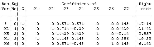
7-15 New Tableau: Proper Form: 7.2-3. " ~ , " ~ c ¬ "Ai ~ 6 c 7 ~ " i ~ 6 c 7 ~ " i ~ c 6 c 7 ~ c 7.2-4. ¬ A ~ b i ‚ b ‚ i ‚ c ‚ c • • °
The current basic solution is superoptimal, but infeasible.
7-16 6 7 " " (a) " ~ c , " ~ ¬ "Ai ~ c ~ " i ~ c 6 c 7 ~ c " i ~ 6 c 7 ~
(b) " ~ c , " ~ c " ~ ¬ "²'i c ³ ~ c b c ~ c i ~ c c 6 c 7 ~ 6c 7 i ~ c 6c 7 ~ c
The current basic solution is feasible, but not optimal.

"
The current basic solution is feasible and optimal.
7-17
(c) " ~ , " ~ " ~ ¬ "²'i c ³ ~ c b ~ " i ~ c ~ 6 7 6 7 i ~ 6 7 ~
The current basic solution is feasible and optimal.
7-18 " i i i (d) " ~ , " ~ " ~ c ¬ "²'i c ³ ~ b ~ " i ~ c ~ c 6 7 6 7 i ~ 6 7 ~
(e) " ~ c ¬ "²' c ³ ~ " ~ c ¬ "²' c ³ ~ " ~ ¬ "²' c ³ ~ c
The current basic solution is feasible, but not optimal.
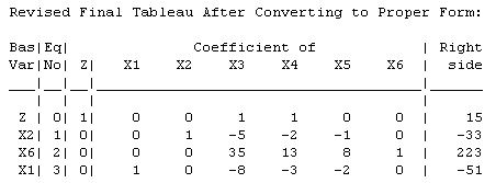
Proper Form:
The current basic solution is infeasible and superoptimal.
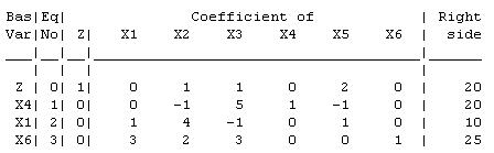
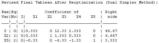
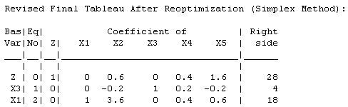
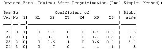
Tableau After Reoptimization:
7-19
(f) New Tableau:
The current basic solution is neither feasible nor optimal.
7-20 " " " " (g) " ~ c , " ~ ¬ "²'i c ³ ~ 6 c 7 ~ c i ~ c 6 c 7 ~ i ~ 6c 7 ~ c ¬ "²'i c ³ ~ 6 7 ~ i ~ c 6 7 ~ c i ~ 6 7 ~ " ~ , " ~ ¬ "Ai ~ 6 7 ~ " i ~ c 6 7 ~ c " i ~ 6 7 ~
7-21 7.2-5. " ~ , " ~ c ¬ "Ai ~ 6 c 7 ~ c " i ~ c 6 c 7 ~ " i ~ 6 Ai² ³ ~ c c 7 ~ c ²% Á% Á% Á% Á% ³ ~ ² c Á Á Á b Á ³ is feasible if c • • . 7.2-6. (a) " ~ c , " ~ , " ~ c pc s ¬ "Ai ~ qc t ~ c " i ~ " i ~ " i ~ pc s qc t pc s qc t pc s qc t ~ c ~ c ~ c
The current basic solution is feasible and optimal. (b)
The current basic solution remains feasible and optimal. (c)
The current basic solution is feasible and optimal.
7-22
" ~ ¬ "²'i c ³ ~ c
¬
c
" ~
"²'i
³ ~ c
The current basic solution remains feasible and optimal.
7-23 (d) " ~ Á " ~ Á " ~ " ~ ¬ "²'i c ³ ~ c b p s p s q t ~ c " i ~ " i ~ " i ~ ~ q t p s ~ q t p s ~ q t
(e) " ~ cÁ " ~ cÁ " ~ " ~ c ¬ "²'i c ³ ~ b pc s c ~ c " i ~ pc s c ~ c q t q t " i ~ pc s c ~ q t " i ~ pc s c ~ c q t " ~ Á " ~ Á " ~
The current basic solution is superoptimal, but infeasible.
7-24 " ~ c ¬ "²'i c ³ ~ b p s p s ~ q t " i ~ " i ~ " i ~ ~ q t p s ~ q t p s ~ q t
The current basic solution is feasible and optimal.
7-25 (f) " ~ ¬ "²'i c ³ ~ c " ~ ¬ "²'i c ³ ~ c " ~ ¬ "²'i c ³ ~ c
" ~ cÁ " ~ Á " ~ pc s ¬ "²'i c ³ ~ q pc s ~ c t " i ~ q ~ c t " i ~ pc s ~ q t " i ~ pc s ~ c q t " ~ Á " ~ Á " ~ p s ¬ "²'i c ³ ~ ~
(g)
7-26 q t
7-27 " i ~ " i ~ " i ~ p s ~ q t p s ~ q t p s ~ q t " ~ Á " ~ Á " ~ p s ¬ "²'i c ³ ~ p s ~ q t " i ~ " i ~ " i ~ ~ q t p s ~ q t p s ~ q t " ~ c , " ~ , " ~ pc s ¬ "Ai ~ q ~ c t " i ~ pc s ~ c q t " i ~ pc s ~ q t " i ~ pc s ~ c q t
The current basic solution is feasible and optimal.

7-28
(h)
The current basic solution is infeasible and superoptimal. Tableau After Reoptimization:
(a) F2-DC, F2-W1 and DC-W2 have the smallest margins for error (100). The greatest effort in estimating the unit shipping costs should be placed on these lanes.
(b)
Cost Allowable Range
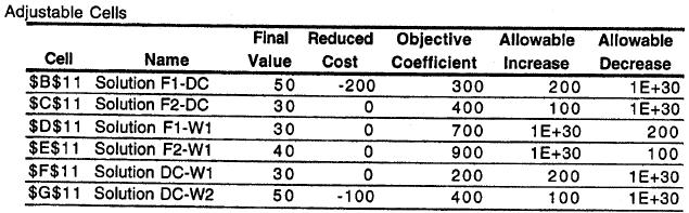
* F1-DC •
* F2-DC •
* F1-W1 ‚
* F2-W1 ‚
* DC-W1 •
* DC-W2 •
(c) The range of optimality for each unit shipping cost indicates how much that shipping cost can change before the optimal shipping quantities change.
(d) Use the 100% rule for simultaneous changes in the objective function coefficients. If the sum of the percentage changes does not exceed 100%, the optimal solution will remain optimal. If it exceeds 100%, then it may or may not be optimal for the new problem.
7-29
7.2-7.
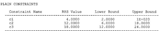
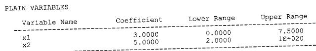
The allowable range for is • • and the one for is c • • c ° .
(b) Increasing by " ( ~ b" )causes the coefficient of % in row 0 of the final tableau to become c" . To make it , add " times row 2 to row 0:
c" b " c ~ b " c" .
For optimality, we need b" ‚ and c" ‚ , so c • " • . Hence, the allowable range for is c ~ • • b ~ Similarly, increasing by "
( ~ c b " )causes the coefficient of % in row 0 of the final tableau to become
c" . To make it , add " times row 1 to row 0:
c" b " c ~ b " c " .
For optimality, we need b" ‚ and c " ‚ , so c • " • ° . Hence, the allowable range for is c c ~c • • c b ° ~c ° .
7-30
7.2-8. (a)
The allowable range for is ‚ .
The allowable range for is • .
(d) If we increase by " , the final right-hand side becomes:
In order to preserve feasibility, " ‚ c , so the allowable range for Similarly, if is increased by " , the final right-hand side becomes: is ‚ .
In order to preserve feasibility, " • , so the allowable range for is • .
7-31 c (c)
:i ~6 c 76
7 ~ 6 7 b 6 7"
b"
.
:i ~ c
b c . 6 c 76 b
7 6 7 6c 7"
~
"
(e) (in MPL)
If we increase by " , the final right-hand side becomes:
Assuming " ~ " ~ , " must satisfy: b " ‚ " ‚ c
c " ‚ " • b " ‚ " ‚ c

c • " • ¯ • •
Assuming " ~ " ~ , " must satisfy:
b " ‚ " ‚ c ‚
Assuming " ~ " ~ , " must satisfy:
b " ‚ " ‚ c
c " ‚ " •
7-32
7.2-9.
p sp b
s i
:i
rc u b
q c tq b" t p s p s p s p s
r u brc u" b " br u" q t q t q t q c t
"
~
~
"
~
7-33 ¯ • • .
The allowable range for is • • .
The allowable range for is ° • .
7-34
The allowable range for is • • 7.2-10.
If we increment by " ( ~ b " ), the coefficient of % in row 0 of the final tableau becomes c" . Add " times row 1 to row 0 to get: 2c" 3 b " ~ 2 b " 3 .
For optimality, we need ² ° ³ b" ‚ , so " ‚ c ° . Hence, the allowable range for is ‚ ° .
The allowable range for is ‚ ° No matter how large gets, ²Á ° ³ stays optimal as long as ‚ ° .
7-35
If we increment by " ( ~ b " ), the coefficient of % in row 0 of the final tableau becomes c" . Add " times row 2 to row 0 to get:
For optimality, we need
, so " ‚ c , so the allowable range for is ‚ . Looking at Figure 6.3, we see that if ~ , A ~ % b % ~ lies exactly on the constraint boundary. Thus, if is decreased any more, ² Á ³ does not remain optimal and the optimal solution becomes ² Á ³. On the other hand, as increases, the objective function gets closer to the horizontal line A ~ % ~ , so for any ‚ , ² Á ³ stays optimal.
7-36 c t q
7.2-11.
2
2 3
² ° ³ b ² ° ³" ‚ and ² ° ³ b ² ° ³" ‚
7.2-12. p c s " p s p s p s (a) i ~r u ‚ b " ‚ q tq " ‚ c ‚ t q t q t p c s p s p s p s i ~ r u " ‚ b r u" ‚ q c tq t q t q c t c • " • • • p c s p c s p s p s i ~r u ‚ b r u" ‚ q c tq" t q t (b) c • " • • • ²Row ³ b " ²Row ³ ‚ c " ‚ and b " ‚ c • " • • • ²Row ³ b " ²Row ³ ‚ b " ‚ c • " •
c" b " b " b " .
3 2 3

7-37 (c)
(in MPL)
7.2-13. p sp b" s p s p s
r i ur u r u r u
r c u
(a) ~ r ur q c tq
" ‚ c ‚ p s
u ‚ r u b r u " ‚ t q t q t s p s p s
p
r r q
i ur b" u r u r u ~ ur tq u ‚ r u b r u " ‚ t q t q t
r c u
" ‚ c ‚ p s s p s p s
r i ur u r u r u
~ r ur u ‚ r u b r u " ‚
c p r c u b "
q c tq
" ‚ c ‚
t q t q t p sp s p s p s
r i ur u r u r u
~ r ur
c u ‚ r u b r c u" ‚
r u r u
q t q t q c t b " q t
c
7-38
7-39 " ‚ c , " • , " • • •
(b) Incrementing by " , the coefficient of % in row 0 of the final tableau becomes ² ° ³c " . In order for the solution to remain optimal, ² ° ³c " ‚ , so
Incrementing by " , the coefficient of % in row 0 of the final tableau becomes c" . Using row 2 to eliminate this coefficient, we get:
To keep optimality, we need:
7-40
• b ~ .
2 3 2 3 c " b
~ 2 b " b " 3
"
.
b " ‚ (c) (in
and b " ‚ " ‚ c ¯ ‚ . 7.2-14. " ~ ¬ "²'i c ³ ~ c " ~ ¬ "²'i c ³ ~ c p " ~ c ¬ "Ai ~ s ~ c p " i ~ c s ~ qc t qc t p " i ~ c s ~ qc t
MPL)
Proper Form:
The current basic solution is feasible and optimal.

7-41 p " i ~ s ~ c
qc t
New Tableau:
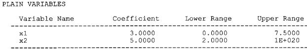
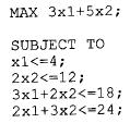
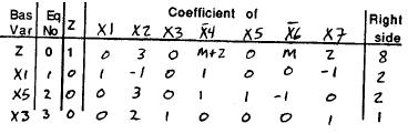
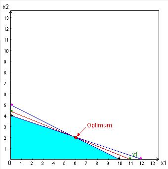
7.3-1. (a) Unit Profit Activity 1 $2.00 Activity 2 $5.00 Resource Usage Resource 1 1 2 Totals 10 Available <= 10 Resource 2 1 3 12 <= 12 Total Profit $22.00 Solution 6 2 Variable Cells Cell Name $B$9 Solution X1 $C$9 Solution X2 Final Reduced Objective Allowable Allowable Value Cost Coefficient Increase Decrease 6 0 2 0 5 0 333333333 2 0 5 1 1
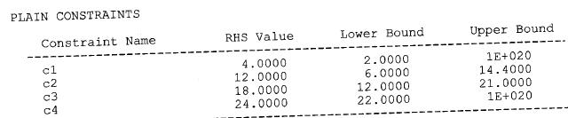
Cell Name Final Value Shadow Price Constraint R H Side Allowable Increase Allowable Decrease $D$5 Constraint 1 Totals 10 1 10 2 2 $D$6 Constraint 2 Totals 12 1 12 3 2
Constraints
(b) The optimal solution is ² Á ³ if the unit profit for Activity 1 is $1.
The optimal solution is ² Á ³ if the unit profit for Activity 1 is $3.
(c) The optimal solution is ² Á ³ if the unit profit for Activity 2 is $2.50.
The optimal solution is ² Á ³ if the unit profit for Activity 2 is $7.50.
7-42
Unit Profit Activity 1 $1.00 Activity 2 $5.00 Resource Usage Resource 1 1 2 Totals 8 Available <= 10 Resource 2 1 3 12 <= 12 Total Profit $20.00 Solution 0 4
Unit Profit Activity 1 $3.00 Activity 2 $5.00 Resource Usage Resource 1 1 2 Totals 10 Available <= 10 Resource 2 1 3 10 <= 12 Total Profit $30 00 Solution 10 0
Unit Profit Activity 1 $2.00 Activity 2 $2.50 Resource Usage Resource 1 1 2 Totals 10 Available <= 10 Resource 2 1 3 10 <= 12 Total Profit $20 00 Solution 10 0
Unit Profit Activity 1 $2.00 Activity 2 $7.50 Resource Usage Resource 1 1 2 Totals 8 Available <= 10 Resource 2 1 3 12 <= 12 Total Profit $30.00 Solution 0 4
The allowable range for the unit profit of Activity 1 is approximately between $1.60 and $1.80 up to between $2.40 and $2.60. The allowable range for the unit profit of Activity 2 is between $3.50 and $4 up to between $5.50 and $6.
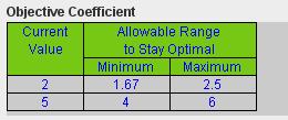
(e) The allowable range for the unit profit of Activity 1 is approximately between $1.67 and $2.50. The allowable range for the unit profit of Activity 2 is between $4 and $6.
(f) The allowable range for the unit profit of Activity 1 is approximately between $1.67 and $2.50. The allowable range for the unit profit of Activity 2 is between $4 and $6.
7-43 (d) Unit Profit for Solution Activity 1 Activity 1 Activity 2 Total Profit $1.00 0 4 $20.00 $1 20 0 4 $20 00 $1 40 0 4 $20 00 $1.60 0 4 $20.00 $1.80 6 2 $20.80 $2 00 6 2 $22 00 $2 20 6 2 $23 20 $2.40 6 2 $24.40 $2.60 10 0 $26.00 $2.80 10 0 $28.00 $3 00 10 0 $30 00 Unit Profit for Solution Activity 2 Activity 1 Activity 2 Total Profit $2.50 10 0 $20.00 $3.00 10 0 $20.00 $3.50 10 0 $20.00 $4.00 6 2 $20.00 $4 50 6 2 $21 00 $5 00 6 2 $22 00 $5 50 6 2 $23 00 $6 00 0 4 $24 00 $6.50 0 4 $26.00 $7.00 0 4 $28.00 $7 50 0 4 $30 00
(h) Keeping the unit profit of Activity 2 fixed, the unit profit of Activity 1 cannot be changed to less than 1.67 or more than 2.5 without changing the optimal solution. Similarly if the unit profit of Activity 1 is fixed at 1, the unit profit of Activity 2 needs to stay between 4 and 6 so that the optimal solution remains the same. Otherwise, the objective function line becomes either too flat or too steep and the optimal solution becomes ² Á ³ or ²
Total Profit Unit Profit for Activity 2 Unit Profit for Activity 1 $2 50 $3 00 $3 50 $4 00 $4 50 $5 00 $5 50 $6 00 $6 50 $7 00 $7 50 $1 00 $11 00 $12 00 $14 00 $16 00 $18 00 $20 00 $22 00 $24 00 $26 00 $28 00 $30 00 $1 20 $12 20 $13 20 $14 20 $16 00 $18 00 $20 00 $22 00 $24 00 $26 00 $28 00 $30 00 $1 40 $14 00 $14 40 $15 40 $16 40 $18 00 $20 00 $22 00 $24 00 $26 00 $28 00 $30 00 $1 60 $16 00 $16 00 $16 60 $17 60 $18 60 $20 00 $22 00 $24 00 $26 00 $28 00 $30 00 $1 80 $18 00 $18 00 $18 00 $18 80 $19 80 $20 80 $22 00 $24 00 $26 00 $28 00 $30 00 $2 00 $20 00 $20 00 $20 00 $20 00 $21 00 $22 00 $23 00 $24 00 $26 00 $28 00 $30 00 $2 20 $22 00 $22 00 $22 00 $22 00 $22 20 $23 20 $24 20 $25 20 $26 20 $28 00 $30 00 $2 40 $24 00 $24 00 $24 00 $24 00 $24 00 $24 40 $25 40 $26 40 $27 40 $28 40 $30 00 $2 60 $26 00 $26 00 $26 00 $26 00 $26 00 $26 00 $26 60 $27 60 $28 60 $29 60 $30 60 $2 80 $28 00 $28 00 $28 00 $28 00 $28 00 $28 00 $28 00 $28 80 $29 80 $30 80 $31 80 $3 00 $30 00 $30 00 $30 00 $30 00 $30 00 $30 00 $30 00 $30 00 $31 00 $32 00 $33 00
7-44 (g)
Á
³
7.3-2.
(a) The original model:
The shadow price (the increase in total profit) is $1.
(b) The shadow price of $1 is valid in the range of to
7-45
Unit Profit Activity 1 $2 00 Activity 2 $5 00 Resource Usage Resource 1 1 2 Totals 10 Available <= 10 Resource 2 1 3 12 <= 12 Total Profit $22.00 Solution 6 2 With one
unit of resource 1: Unit Profit Activity 1 $2.00 Activity 2 $5.00 Resource Usage Resource 1 1 2 Totals 11 Available <= 11 Resource 2 1 3 12 <= 12 Total Profit $23.00 Solution 9 1
additional
Available Solution Total Incrementa l Resource 1 Activity 1 Activity 2 Profit Profit 5 0 2 5 $12 50 6 0 3 $15 00 $2 50 7 0 3 5 $17 50 $2 50 8 0 4 $20 00 $2 50 9 3 3 $21 00 $1 00 10 6 2 $22 00 $1 00 11 9 1 $23 00 $1 00 12 12 0 $24.00 $1.00 13 12 0 $24 00 $0 00 14 12 0 $24.00 $0.00 15 12 0 $24 00 $0 00