Swaps: The $37 Trillion Market

NOBEL PERSPECTIVES: WASSILY LEONTIEF: INPUT OUTPUT MODELS

An old economics professor always would start his principles classes by telling his students a trite story about some average person living in NYC: The person got up every morning at 7:00, drank several cups of coffee to wake up, drove to work, labored for eight hours, drove home, and so on. The professor would then tell his students that if they wanted to make the story more interesting, then they should consider the fact that there are millions of people in NYC, along with over 150 million people in the United States, who do roughly the same things every day. He then asked them the question: How is it that an economic system knows how to produce just enough coffee to wake everyone up, just enough gas to get people back and forth to work, and so on? The students would later discover that the answer lies in understanding how a market-oriented, capitalistic system works.

The professor would go on to explain that the study of economics focuses on explaining how complex systems function by developing models. Economist Fritz Machlup defined models such as Keynes’ General Equilibrium Model and Solow’s Growth Theory as abstractions of complex phenomenon. However, Russian economist Wassily Leontief (1906–1999) believed it was impossible to understand an economy by studying it in abstraction. In the 1930s, Leontief developed the Input-Output Model: a general model of production based on economic interdependence. He later expanded the theory by generating the first empirical input-output model. Leontief’s Input-Output Model is a matrix-based framework that explains the outputs of one industry as inputs to other industries and final demand. $0.398 increase in manufacturing output, a $1.004 increase in construction sector output, and a $0.122 increase in professional services; which means a $1.00 increase in construction results in a total increase in aggregate output of $1.485. Economists have also used the direct/indirect matrix to forecast sector outputs based on expected demand in each sector and to study the impact of policy changes.

Today, there are input-output models disaggregated into as many as 300 subsectors, regional and state models, and country models. These models have proved to be crucial in understanding the economies of the world and how they are interconnected through global supply chains. Leontief himself used his model to test the Heckscher-Ohlin theory. This classic theory held that capital-abundant countries like the United States gain by exporting relatively more capital-intensive commodities and importing more labor-intensive goods. However, Leontief, in examining the input-output structure of the U.S. economy found just the opposite —Leontief Paradox. Input-output models also provide the framework for many of today’s supply-chain models. One of the most sophisticated of these models is Bloomberg’s supply chain platform. The platform provides a comprehensive supply chain breakdown for thousands of publicly traded companies. For example, Bloomberg’s supply chain platform for Apple Inc. shows that Apple has 343 suppliers and 166 customers. Apple pays 49.67% of their cost of goods sold to Hon Hai Precision, 14.09% to the Pegatron Corporation, and 10.23% to Quanta Computer. Among Apple’s customer, 3.80% of its revenue comes from sales to AT&T, 2.46% from Best Buy, and 2.17% from China Mobil (Table 2).

The direct table shows the amount of sector inputs needed to produce $1.00 of a sector’s output. For exam- In 1996, a graduate student at Stanford University deveple, the 2015 U.S. input-output model shows that to loped an algorithm that ranked the popularity of pages produce $1.00 of manufacturing goods, the manufactu- appearing on the worldwide web. The algorithm is known ring sector buys $0.045 from itself, $0.056 from the as the “Page Rank Algorithm” and the author is Larry mining sector, $0.075 of professional services, $0.158 for Page, co-founder of Google. Interestingly, the algorithm labor employment, and spends $0.014 in taxes. In the uses a methodology similar to the one used by Leontief to direct matrix, each row shows the sales of that sector to develop his input-output model. Leontief taught four other sectors. The direct/indirect table, in turn, shows doctoral students, who were awarded the Nobel Prize in the total output requirements needed to meet final sector Economic Science: Paul Samuelson, 1970, Robert Solow, demands. For example, in order to produce say $1.00 of 1987, Vernon L. Smith, 2002, and Thomas Schelling, construction goods, the table factors in both the direct 2005. Wassily Leontief was himself awarded the Nobel and indirect input requirements needed by each sector to Prize in Economic Sciences in 1973 for his work on the generate the $1.00 of output. Thus, the product of multi- Input-Output model—a model that goes far in helping us plying the matrix by each sector’s final demand equals understand how an economic system knows how to the total output of each individual sector. The direct-indi- produce just enough coffee to wake everyone up, just rect matrix is particularly useful in conducting impact enough gas to get people back and forth to work, and so assessments. on. For instance, using the 2015 U.S. input-output model, a $1.00 increase in construction demand would lead to a

Source: U.S. Bureau of Economic Analysis

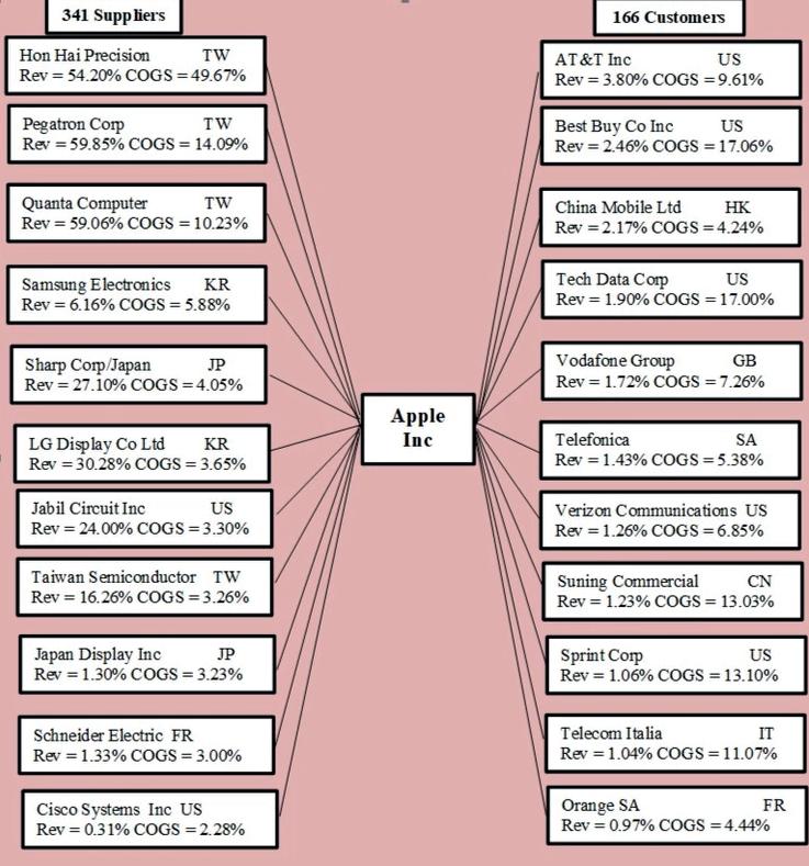
Table 1: U.S. Input-Output Model

Table 2: Apple Inc. Supply Chain Source: Bloomberg

SWAPS: THE $37 TRILLION MARKET

Financial Innovation Series

Over the past 50 years, the investment industry has seen stock market and real estate bubbles, interest rates approaching zero, the emergence of hedge funds and private equity companies, the globalization of financial markets, the proliferation of derivative securities, and the growth of securitized assets and structured financing. Mirroring these events has been the academic contributions to the investment discipline: the development of capital market theories, the derivation of option pricing models, and the explorations into efficient market theories. The financial events and the academic contributions together highlight what is truly an innovative financial industry. In this article, we examine one of the most significant industry innovations in the last forty years— the rise of the $37 trillion swap.

In 1981, Germany and Switzerland limited the World Bank from borrowing German marks and Swiss francs to finance its operations. IBM, on the other hand, had already borrowed large amounts of those currencies but needed U.S. dollars. To resolve this problem, Salomon Brothers arranged a swap in which IBM traded its borrowed francs and marks for the World Bank’s dollars. Many observers point to this World Bank and IBM currency swap as the agreement that propelled the tremendous growth that occurred in the currency swap markets over the last four decades. Today, it is common for corporations and financial institutions to exchange loans denominated in different currencies, creating a $21 trillion currency swap market. A year after the World Bank and IBM swap, the Student Loan Marketing Association (Sallie Mae) issued a fixed-rate, intermediate-term bond through a private placement and swapped it for a floating-rate note issued by the ITT Corporation. This exchange of the floating-rate loan for the fixed-rate one represented the first interest rate swap. The swap provided ITT with fixed-rate funds at a rate below the rate they could obtain on a direct fixed-rate loan, and it provided Sallie Mae with cheaper intermediate-term, floating-rate funds – both parties, therefore, benefited from the swap.

Today, there exists a $14.7 trillion interest rate swap market consisting of financial and non-financial corporations who annually conduct (as measured by contract value) swaps of fixed-rate loans for floating-rate loans. Financial institutions and corporations use the market to hedge their liabilities and assets more efficiently – transforming their floating-rate liabilities and assets into fixed-rate ones or vice versa and creating synthetic fixed or floating-rate liabilities and assets with better rates than the ones they can directly obtain. Concomitant with the growth of interest rate and currency swaps there has been a number of innovations introduced in swaps contracts over the years. Today, there are several non-generic swaps used by financial and non-financial corporations to structure their liability and asset positions.

Over the last decade, one of the most popular swaps has been the credit default swap. Introduced by JP Morgan in 1994, this swap allows companies to trade credit risk and by so doing change their debt and fixed-income assets credit risk exposure. During the 2008 financial crisis, credit default swaps on mortgage-backed securities were one of the contributing factors to the economic downturn. Whether it is an exchange of currency-denominated loans, fixed and floating interest rate payments, or payments of insurance premiums for credit protection, a swap, by definition, is a legal arrangement between two parties to exchange specific payments. This article examines this $37 trillion swap market.

INTEREST RATE SWAPS

The simplest type of interest rate swap is the plain vanilla or generic swap. In this agreement, one party provides fixed-rate interest payments to another who provides floating-rate payments. The parties to the agreement are referred to as counterparties. The party who pays fixed interest and receives floating is the fixed-rate payer; the other party (who pays floating and receives fixed) is the floating-rate payer. On a generic swap, principal payments are not exchanged. As a result, the interest payments are based on a notional principal (NP).

The interest rate paid by the fixed payer often is specified in terms of the yield to maturity (YTM) on a T-note plus basis points; the rate paid by the floating payer on a generic swap is the London Interbank Offer Rate, LIBOR (a short-term rate often used to set rates on floating rate debt). Swap payments on a generic swap are semiannual and the original maturities typically range from three to 10 years. In the swap contract, the effective date is the date when interest begins to accrue; the settlement or payment date is when interest payments are made (interest is paid in arrears six months after the effective date). On the payment date, only the interest differential between the counterparties is paid. Thus, if a fixed-rate payer owes $3 million and a floating-rate payer owes $2.5 million, then only a $0.5 million payment by the fixed payer to the floating payer is made. To illustrate, consider a 3.5% fixed rate for floating rate swap with a notional principal of $10 million, maturity of three years, starting on 3/15/Y1, and maturing on 3/15/Y4. In this swap agreement, the fixed-rate payer agrees to pay the current yield on a three-year T-note of 3.5% and the floating-rate payer agrees to pay the 6-month LIBOR as determined on the effective dates with no basis points,