11.12 Correlation
433
0.6
0.6
•
« • •• • • •
• • -0.3
0.3
•
* •
-0.6
•
•
0.3
*
•
• •
•
•
• •
• • -0.3
•
•
-0.6 20
15 Density
10
25
-2
-1 0 1 Standard Normal Quantile
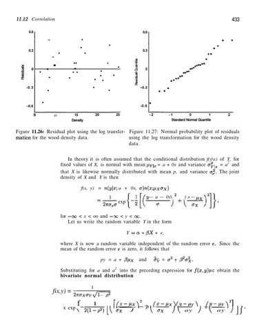
Figure 11.26: Residual plot using the log transfer- Figure 11.27: Normal probability plot of residuals mation for the wood density data. using the log transformation for the wood density data. In theory it is often assumed that the conditional distribution f(y\x) of Y, for fixed values of X, is normal with mean p.y\x = a + 0x and variance Oy<x = a2 and that X is likewise normally distributed with mean p, and variance a2. The joint density of X and Y is then f(x, y) = n(y\x; a + 0x, a)n(x; px, ax) (y — a — 0x\
1 2itaxa exp
(x
Px o~x
for —oo < x < oo and —oc < y < ex. Let us write the random variable Y in the form Y = a + BX + e, where X is now a random variable independent of the random error e. Since the mean of the random error e is zero, it follows that py = a + 0px
ay = a2 + 02a\.
and
Substituting for a and a2 into the preceding expression for fix,y), we obtain the bivariate normal distribution
fix,y) =
1 27TCT,Yay y/\ — O2
f x exp \
l 2(l-(fi)[\
\(x-px\2 _ 2P fx-px\ (y-PY\ ax
J
\
crx
J\
ay
(V-PYV] J
+
{
ay
1 )\f>