
Solutions Manual to Principles of Electronic Materials and Devices
Fourth Edition
© 2018 McGraw-Hill
CHAPTER 2
Safa Kasap
University of Saskatchewan
Canada
Check author's website for updates
http://electronicmaterials.usask.ca
NOTE TO INSTRUCTORS
If you are posting solutions on the internet, you must password the access and download so that only your students can download the solutions, no one else. Word format may be available from the author. Please check the above website. Report errors and corrections directly to the author at safa.kasap@yahoo.com
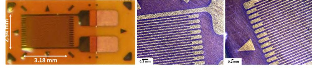
A commercial strain gauge by Micro- Measurements (Vishay Precision Group). This gauge has a maximum strain range of ±5%. The overall resistance of the gauge is 350 Ω. The gauge wire is a constantan alloy with a small thermal coefficient of resistance. The gauge wires are embedded in a polyimide polymer flexible substrate. The whole gauge is fully encapsulated in the polyimide polymer. The external solder pads are copper coated. Its useful temperature range is –75 °C to +175 °C.
Copyright © McGraw-Hill Education. All rights reserved. No reproduction or distribution without the prior written consent of McGraw-Hill Education.
Chapter 2
Answers to "Why?" in the text
Page 187, footnote 21
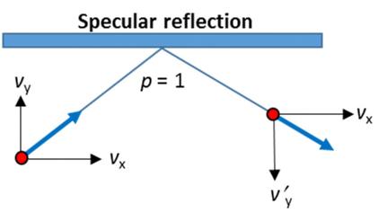
Figure below shows specular reflection, that is, a totally elastic collision of an electron with the surface of a film. If this were a rubber ball bouncing off a wall, then there would only be a change in the ycomponent vy of the velocity, which would be reversed. The x-component is unchanged. The collision has no effect on the vx component of the velocity. If there is an electric field in the x direction then the electron can continue to gain velocity from the field as if it never collided with the wall. Specular reflection does not increase the resistivity.
Page 196, footnote 21
"Pure Al suffers badly from electromigration problems and is usually alloyed with small amounts of Cu, called Al(Cu), to reduce electromigration to a tolerable level. But the resistivity increases. (Why?)" The increase is due to Matthiessen's rule. The added impurities (Cu) in Al provide an additional scattering mechanism.
2.1 Electrical conduction Na is a monovalent metal (BCC) with a density of 0.9712 g cm 3. Its atomic mass is 22.99 g mol 1. The drift mobility of electrons in Na is 53 cm2 V 1 s 1 .
a. Consider the collection of conduction electrons in the solid. If each Na atom donates one electron to the electron sea, estimate the mean separation between the electrons. (Note: if n is the concentration of particles, then the particles’ mean separation d = 1/n1/3.)
b. Estimate the mean separation between an electron (e ) and a metal ion (Na+), assuming that most of the time the electron prefers to be between two neighboring Na+ ions. What is the approximate Coulombic interaction energy (in eV) between an electron and an Na+ ion?
c. How does this electron/metal-ion interaction energy compare with the average thermal energy per particle, according to the kinetic molecular theory of matter? Do you expect the kinetic molecular theory to be applicable to the conduction electrons in Na? If the mean electron/metal-ion interaction energy is of the same order of magnitude as the mean KE of the electrons, what is the mean speed of electrons in Na? Why should the mean kinetic energy be comparable to the mean electron/metal-ion interaction energy?
Copyright © McGraw-Hill Education. All rights reserved. No reproduction or distribution without the prior written consent of McGraw-Hill Education.
d. Calculate the electrical conductivity of Na and compare this with the experimental value of 2.1 × 10⁷ Ω 1 m 1 and comment on the difference.
Solution
a. If D is the density, Mat is the atomic mass and NA is Avogadro's number, then the atomic concentration
is
which is also the electron concentration, given that each Na atom contributes 1 conduction electron. If d is the mean separation between the electrons then d and nat are related by (see Chapter 1 Solutions, Q1.11; this is only an estimate)
b. Na is BCC with 2 atoms in the unit cell. So if a is the lattice constant (side of the cubic unit cell), the density is given by
cell)(mass
cell unit of volume
nm
For the BCC structure, the radius of the metal ion R and the lattice parameter a are related by (4R)2 = 3a2, so that,
If the electron is somewhere roughly between two metal ions, then the mean electron to metal ion separation delectron-ion is roughly R. If delectron-ion ≈ R, the electrostatic potential energy PE between a conduction electron and one metal ion is then
c. This electron-ion PE is much larger than the average thermal energy expected from the kinetic theory for a collection of “free” particles, that is Eaverage = KEaverage = 3(kT/2) ≈ 0.039 eV at 300 K. In the case of Na, the electron-ion interaction is very strong so we cannot assume that the electrons are moving around freely as if in the case of free gas particles in a cylinder. If we assume that the mean KE is roughly the same order of magnitude as the mean PE,
Copyright © McGraw-Hill Education. All rights reserved. No reproduction or distribution without the prior written consent of McGraw-Hill Education.
There is a theorem in classical physics called the Virial theorem which states that if the interactions between particles in a system obey the inverse square law (as in Coulombic interactions) then the magnitude of the mean KE is equal to the magnitude of the mean PE. The Virial Theorem states that:
Indeed, using this expression in Eqn. (2), we would find that u = 1.05 × 10⁶ m/s. If the conduction electrons were moving around freely and obeying the kinetic theory, then we would expect (1/2)meu2 = (3/2)kT and u = 1.1 × 10⁵ m/s, a much lower mean speed. Further, kinetic theory predicts that u increases as T1/2 whereas according to Eqns. (1) and (2), u is insensitive to the temperature. The experimental linear dependence between the resistivity ρ and the absolute temperature T for most metals (non-magnetic) can only be explained by taking u = constant as implied by Eqns. (1) and (2).
d. If µ is the drift mobility of the conduction electrons and n is their concentration, then the electrical conductivity of Na is σ = enµ Assuming that each Na atom donates one conduction electron (n = nat), we have
which is quite close to the experimental value.
Nota Bene: If one takes the Na+-Na+ separation 2R to be roughly the mean electron-electron separation then this is 0.37 nm and close to d = 1/(n1/3) = 0.34 nm. In any event, all calculations are only approximate to highlight the main point. The interaction PE is substantial compared with the mean thermal energy and we cannot use (3/2)kT for the mean KE!
2.2 Electrical conduction The resistivity of aluminum at 25 °C has been measured to be 2.72 × 10 8 Ω m. The thermal coefficient of resistivity of aluminum at 0 °C is 4.29 × 10 3 K 1. Aluminum has a valency of 3, a density of 2.70 g cm 3, and an atomic mass of 27.
a Calculate the resistivity of aluminum at 40ºC
b. What is the thermal coefficient of resistivity at ─40ºC?
c. Estimate the mean free time between collisions for the conduction electrons in aluminum at 25 °C, and hence estimate their drift mobility.
d. If the mean speed of the conduction electrons is about 2 × 10⁶ m s 1, calculate the mean free path and compare this with the interatomic separation in Al (Al is FCC). What should be the thickness of an Al film that is deposited on an IC chip such that its resistivity is the same as that of bulk Al?
e. What is the percentage change in the power loss due to Joule heating of the aluminum wire when the temperature drops from 25 °C to 40 ºC?
Solution
a. Apply the equation for temperature dependence of resistivity, ρ(T) = ρo[1 + αo(T To)]. We have the temperature coefficient of resistivity, αo, at To where To is the reference temperature. We can either work in K or °C inasmuch as only temperature changes are involved. The two given reference temperatures are 0 °C or 25 °C, depending on choice. Taking To = 0 °C,
ρ( 40°C) = ρo[1 + αo( 40°C 0°C)]
ρ(25°C) = ρo[1 + αo(25°C 0°C)]
Divide the above two equations to eliminate ρo,
ρ( 40°C)/ρ(25°C) = [1 + αo( 40°C)] / [1 + αo(25°C)]
Next, substitute the given values ρ(25°C) = 2.72 × 10 8 Ω m and αo = 4.29 × 10 3 K 1 to obtain
b. In ρ(T) = ρo[1 + αo(T To)] we have αo at To where To is the reference temperature, for example, 0° C or 25 °C depending on choice. We will choose To to be first at 0 °C and then at 40 °C (= T2) so that the resistivity at T2 and then at To are:
At T2, ρ2 = ρo[1 + αo(Τ2 Το)]; the reference being To and ρo which defines αo and at To ρo = ρ2[1 + α2(Το Τ2)]; the reference being T2 and ρ2 which defines α2
Rearranging the above two equations we find
α2 = αο / [1 + (Τ2 Τo)αο]
i.e. α 40 = (4 29 × 10 3) / [1 + ( 40 0)(4 29 × 10 3)] = 5 18 × 10 3 °C 1
Alternatively, consider the definition of α2 that is α 40
From oT o o dT d = ρ ρ α 1
we have α 40 ={1/[ρ( 40 °C)]} × {[ρ(25°C) ρ( 40°C)] / [(25°C) ρ( 40°C)]}
∴ α-40 = 1 / [(2.035 × 10 8)] × {(2 72 × 10 8) (2 035 × 10 8)] / [(25) ( 40)]}
∴ α-40 = 5.18 × 10 3 K 1
c. We know that 1/ρ = σ = enµ where σ is the electrical conductivity, e is the electron charge, and µ is the electron drift mobility. We also know that µ = eτ / me, where τ is the mean free time between electron collisions and me is the electron mass. Therefore,
Copyright © McGraw-Hill Education. All rights reserved. No reproduction or distribution without the prior written consent of McGraw-Hill Education.
Here n is the number of conduction electrons per unit volume. But, from the density d and atomic mass Mat, atomic concentration of Al is
so that n = 3nAl = 1.807 × 10
assuming that each Al atom contributes 3 "free" conduction electrons to the metal and substituting into (1),
(Note: If you do not convert to meters and instead use centimeters you will not get the correct answer because seconds is an SI unit.)
The relation between the drift mobility
mean free time is given by Equation 2.5, so that
d. The mean free path is
where
is the mean speed. With
we find the mean free path:
A thin film of Al must have a much greater thickness than l to show bulk behavior. Otherwise, scattering from the surfaces will increase the resistivity by virtue of Matthiessen's rule.
e. Power P = I2R and is proportional to the resistivity ρ, assuming the rms current level stays relatively constant. Then we have
(Negative sign means a reduction in the power loss).
2.3 Conduction in gold Gold is in the same group as Cu and Ag. Assuming that each Au atom donates one conduction electron, calculate the drift mobility of the electrons in gold at 22° C. What is the mean free path of the conduction electrons if their mean speed is 1.4 × 10⁶ m s 1? (Use ρo and αo in Table 2.1.)
Solution
The drift mobility of electrons can be obtained by using the conductivity relation σ = enµd
Copyright © McGraw-Hill Education. All rights reserved. No reproduction or distribution without the prior written consent of McGraw-Hill Education.
Resistivity of pure gold from Table 2.1 at 0°C (273 K) is ρ0 = 20.50 nΩ m. Resistivity at 20 °C can be calculated by.
The TCR α0 for Au from Table 2.1 is 1/242 K 1. Therefore the resistivity for Au at 22°C is
20.50
Since one Au atom donates one conduction electron, the electron concentration is
Note: The lattice parameter for Au (which is FCC), a = 408 pm or 0.408 nm. Thus l/a = 92. The electron traveling along the cube edge travels for 92 unit cells before it is scattered.
2.4 Mean free time between collisions Let 1/τ be the mean probability per unit time that a conduction electron in a metal collides with (or is scattered by) lattice vibrations, impurities or defects etc. Then the probability that an electron makes a collision in a small time interval δt is δt/τ. Suppose that n(t) is the concentration of electrons that have not yet collided. The change δn in the uncollided electron concentration is then nδt/τ. Thus, δn = nδt/τ, or δn/n = δt/τ. We can integrate this from n = no at x = 0 to n = n(t) at time t to find the concentration of uncollided electrons n(t) at t
n(t) = noexp( t/τ)
Concentration of uncollided electrons [2.85]
Show that the mean free time and mean square free time are given by
What is your conclusion?
Solution Consider
Copyright © McGraw-Hill Education. All rights reserved. No reproduction or distribution without the prior written consent of McGraw-Hill Education.
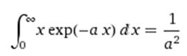
The last term can be integrated by parts (for example, online at http://www.wolframalpha.com) to find, or in terms of the integration limits, that is, as a definite integral,
Thus, Equation (1) becomes
Now
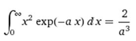
The definite integral can be evaluated or looked up (for example online at http://www.wolframalpha.com)
Thus Equation (2) becomes,
2.5 Effective number of conduction electrons per atom
a. Electron drift mobility in tin (Sn) is 3.9 cm2 V 1 s 1. The room temperature (20 °C) resistivity of Sn is about 110 nΩ m. Atomic mass Mat and density of Sn are 118.69 g mol 1 and 7.30 g cm 3 , respectively. How many “free” electrons are donated by each Sn atom in the crystal? How does this compare with the position of Sn in Group IVB of the Periodic Table?
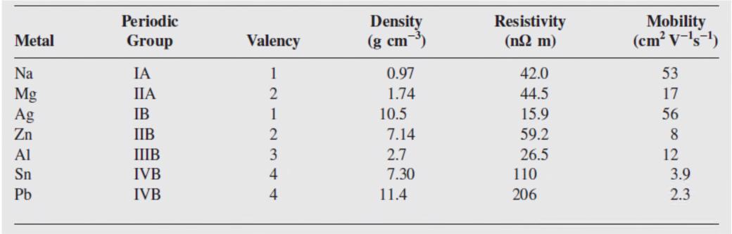
b. Consider the resistivity of few selected metals from Groups I to IV in the Periodic Table in Table 2.8. Calculate the number of conduction electrons contributed per atom and compare this with the location of the element in the Periodic Table. What is your conclusion?
Table 2.8 Selection of metals from Groups I to IV in the Periodic Table
NOTE: Mobility from Hall-effect measurements.
Solution
a. Electron concentration can be calculated from the conductivity of Sn, σ = enµd
= 3.70 × 1028 Sn atoms m 3 .
Hence the number of electrons donated by each atom is (ne/nat) = 3.94 or 4 electrons per Sn atom. This is in good agreement with the position of the Sn in the Periodic Table (IVB) and its valency of 4.
b. Using the same method used above, the number of electrons donated by each atom of the element are calculated and tabulated as follows in Table 2Q05.
Table
Copyright © McGraw-Hill Education. All rights reserved. No reproduction or distribution without the prior written consent of McGraw-Hill Education.
As evident from the above table, the calculated number of electrons donated by one atom of the element is the same as the valency of that element and the position in the periodic table.
Table 2Q05 Number of electrons donated by various elements in Excel
2.6 Resistivity of Ta Consider the resisitivity of tantalum, which is summarized in Table 2.9. Plot ρ against T on a log-log plot and find n for the behavior ρ ∝Tn. Find the TCR at 0 and 25 °C. What is your conclusion? (Data from the CRC Handbook of Chemistry and Physics, 96th Edition, 2015-2016)
Table 2.9 Resistivity of Ta
Figure 2Q06-1 shows a plot of resistivity vs. temperature on a log-log plot, from Excel. On a log-log plot, the "best line" is a power law fit on a log-log plot. The best power law fit generates
Copyright © McGraw-Hill Education. All rights reserved. No reproduction or distribution without the prior written consent of McGraw-Hill Education.
y = 0.3642x1.034
R² = 0.9987
*2.7 TCR of isomorphous alloys Determine the composition of the Cu-Ni alloy that will have a TCR of 4×10 4 K 1, that is, a TCR that is an order of magnitude less than that of Cu. Over the composition range of interest, the resistivity of the Cu-Ni alloy can be calculated from ρCuNi ≈ ρCu + Ceff X (1-X), where Ceff, the effective Nordheim coefficient, is about 1310 nΩ m. Solution
Assume room temperature T = 293 K. Using values for copper from Table 2.1 in Equation 2.19, ρCu = 17.1 nΩ m and αCu = 4.0 × 10 3 K 1, and from Table 2.3 the effective Nordheim coefficient of Ni dissolved in Cu is C = 1310 nΩ m. We want to find the composition of the alloy such that αCuNi = 4 × 10 4 K 1. Then,

Using Nordheim’s rule:
Copyright © McGraw-Hill Education. All rights reserved. No reproduction or distribution without the prior written consent of McGraw-Hill Education.
ρalloy = ρCu + CX(1 X)
i.e. 171.0 nΩ m = 17.1 nΩ m + (1310 nΩ m)X(1 X)
∴ X2 X + 0.1175 = 0
solving the quadratic, we find X = 0.136
Thus the composition is 86.4% Cu-13.6% Ni. However, this value is in atomic percent as the Nordheim coefficient is in atomic percent. Note that as Cu and Ni are very close in the Periodic Table this would also be the weight percentage. Note: the quadratic will produce another value, namely X = 0.866. However, using this number to obtain a composition of 13.6% Cu-86.4% Ni is incorrect because the values we used in calculations corresponded to a solution of Ni dissolved in Cu, not vice-versa (i.e. Ni was taken to be the impurity).
Note: From the Nordheim rule, the resistivity of the alloy is ρalloy = ρο + CX(1 X). We can find the TCR of the alloy from its definition
To obtain the desired equation, we must assume that C is temperature independent (i.e. the increase in the resistivity depends on the lattice distortion induced by the impurity) so that d[CX(1 X)]/dT = 0, enabling us to substitute for dρo/dT using the definition of the TCR: αo =(dρo/dT)/ρo. Substituting into the above equation:
Remember that all values for the alloy and pure substance must all be taken at the same temperature, or the equation is invalid.
Comment: Nordheim's rule does not work particularly well for alloys in which one or both elements are transition metals. Its applicability in alloys that involve a transition metal is only approximate as mentioned in the text. The alloy resistivity in these cases is given by
ρalloy = ρCu + CX(1 X) + ρs-d where ρs-d is an additional resistivity term arising from additional scattering mechanism due to the addition of transition metals. This term depends on X2(1 X), which has been neglected. Its inclusion does not dramatically change the results.
2.8 Resistivity of isomorphous alloys and Nordheim’s rule What are the maximum atomic and weight percentages of Cu that can be added to Au without exceeding a resistivity that is twice that of pure gold? What are the maximum atomic and weight percentages of Au that can be added to pure Cu without exceeding twice the resistivity of pure copper? (Alloys are normally prepared by mixing the elements in weight.)
Solution
Cu added Au
Copyright © McGraw-Hill Education. All rights reserved. No reproduction or distribution without the prior written consent of McGraw-Hill Education.
From combined Matthiessen and Nordheim rule, ρAlloy =ρAu + ρI, with ρI = CX(1 X) is the increase in resistivity dues to Cu addition (impurities). In order to keep the resistivity of the alloy less than twice of pure gold, the resistivity of solute (Cu), should be less than resistivity of pure gold, i.e. ρI = CX(1 X) < ρAu. From Table 2.3, Nordheim coefficient for Cu in Au at 20°C is C = 450 nΩ m. Resistivity of Au at 20°C, using α0 = 1/242 K 1 in Table 2.1 is
Therefore the condition for solute (Cu) atomic fraction is ρAlloy =ρAu + ρI < 2ρAu
∴
ρI < ρAu or CX(1 X) < 22.2 nΩ m.
∴ X(1 X) < (22.2 nΩ m) /(450 nΩ m) = 0.0493
Consider the equality case, the maximum Cu addition, X2 – X + 0.0493 = 0
Solving the above equation, we have X = 0.052 or 5.2% (atomic). Therefore the atomic fraction of Cu should be less than 0.052 or 5.2% in order to keep the overall resistivity of the alloy less than twice the resistivity of pure Au. The weight fraction for Cu for this atomic fraction can be calculated from
= 0.0174 or 1.74% (weight).
Au added to Cu
Now, we discuss the case of Au in Cu, i.e. Au as solute in Cu alloy. Resistivity of Cu at 0°C is 15.4 nΩ m (Table 2.1) and α0 = 1/(235 K). Therefore the resistivity of Cu at 20°C is
Therefore the condition for solute (Au) atomic fraction is ρI = CX(1 X) < ρCu = 17.03 nΩ m. The Nordheim coefficient for Au in Cu at 20°C is, C = 5500 nΩ m. Consider the equality case, the maximum Au addition case,
X(1 X) = (16.71 nΩ m) / (5500 nΩ m) = 3.04×10 3 . X2 – X – 3.04×10 3 = 0
Solving the above equation, we get X = 3.05×10 3 or 0.30 % (atomic) for the maximum Au content we can add. Thus, the Au content has to be less than 0.30% (atomic percent) to keep the resistivity of alloy less than twice of pure Cu. The weight fraction for Cu for this atomic fraction can be calculated from
Copyright © McGraw-Hill Education. All rights reserved. No reproduction or distribution without the prior written consent of McGraw-Hill Education.
9.35 ×10 3 or 0.935% (weight).
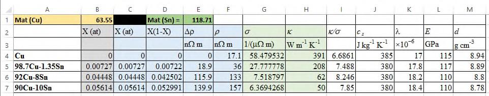
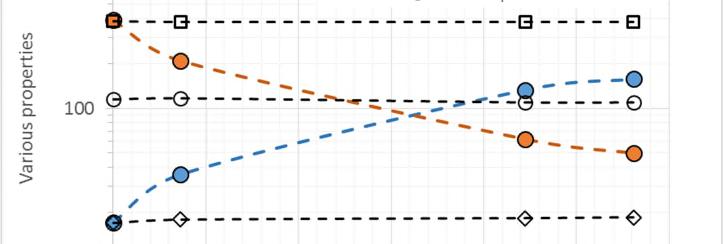
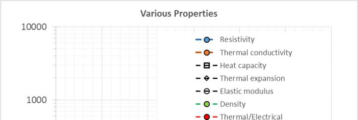
2.9 Physical properties of alloys Consider Cu-Sn alloys, called phosphor bronze. Their properties are listed in Table 2.10 from the ASM Handbook. Plot these properties all in graph (using a log-scale for the properties axis) as a function of composition and deduce conclusions. How does κ/σ change? Compositions are wt. %. Assume the Cu-Sn is a solid solution over this composition range.
Table 2.10 Selected properties of Cu with Sn at 20
Note: ρ is resistivity, κ is thermal conductivity, cs is specific heat capacity, λis linear expansion coefficient, E is Young's modulus and d is density.
We can convert wt% to at.% using The atomic fractions of the constituents can be calculated using the relations proved above. The atomic masses of the components are MSn = 118.71 g mol
mol 1.Applying the weight to atomic fraction conversion equation derived in Ch.
for
= 63.54
case
Other values are listed in table 2Q09-1
Copyright © McGraw-Hill Education. All rights reserved. No reproduction or distribution without the prior written consent of McGraw-Hill Education.
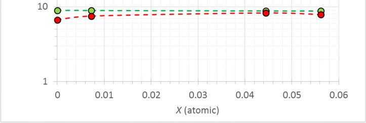
Figure 2Q09-1 shows various properties of Cu-Sn alloys as a function of Sn content in atomic percent. Clearly there are strong changes in the electrical resistivity and thermal conductivity whereas cs, λ, E and d are hardly affected at all. The alloy retains metallic bonding, the Cu crystal structure and is a solid solution so there are no major changes in bonding or the crystal structure with up to ~ 5.6 at.% Sn added. The reason both electrical and thermal conductivity are affected strongly is that both depend on the motion of conduction electrons and how these are scattered. The introduction of foreign impurities that provide an additional scattering mechanism increases the resistivity per Matthiessen's rule.
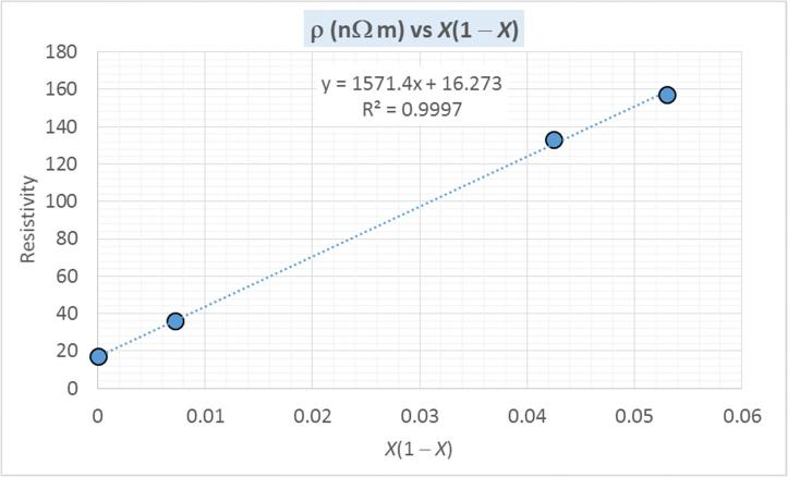
Figure 2Q09-2 shows a plot of the resistivity vs. X(1 X), and it is clearly a straight line with a slope
Slope = C = 1571 nΩ m
This is smaller than the value of C quoted in Table 2.1, which is taken from a handbook (1982).
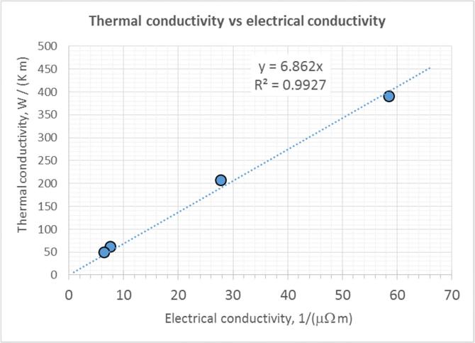
We can also plot κ vs. σ as in Figure 2Q09-3. Clearly κ is proportional to σ as we expect from the Wiedemann-Franz-Lorenz law. The best fit line passing through the origin and gives a slope of
Slope = CWFLT = 6.862×10 6 so that
CWFL = (6.862×10 6) / (300) = 2.30×10 8 W Ω K 2 .
This value is about 5.7% different than the expected value in Equation 2.42.
NOTE: "Tin bronzes, with up 15.8% tin, retain the structure of alpha copper. The tin is a solid solution strengthener in copper, even though tin has a low solubility in copper at room temperature. The room temperature phase transformations are slow and usually do not occur, therefore these alloys are single phase alloys." From: The Website of the Copper Development Associate (https://www.copper.org/resources/properties/microstructure/cu_tin.html) accessed October 4, 2016
Note: The problem emphasizes the importance of electron scattering in controlling ρ and κ. Normally Cu-Sn phase diagram shows a very small solubility limit for Sn but, as explained above, these compositions are single phase solid solutions.
Copyright © McGraw-Hill Education. All rights reserved. No reproduction or distribution without the prior written consent of McGraw-Hill Education.
Copyright © McGraw-Hill Education. All rights reserved. No reproduction or distribution without the prior written consent of McGraw-Hill Education.
2.10 Nordheim’s rule and brass Brass is a Cu–Zn alloy. Table 2.11 shows some typical resistivity values for various Cu–Zn compositions in which the alloy is a solid solution (up to 30% Zn).
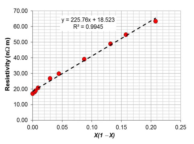
a. Plot ρ versus X(1 X). From the slope of the best-fit line find the mean (effective) Nordheim coefficient C for Zn dissolved in Cu over this compositional range.
b. Since X is the atomic fraction of Zn in brass, for each atom in the alloy, there are X Zn atoms and (1X) Cu atoms. The conduction electrons consist of each Zn donating two electrons and each copper donating one electron. Thus, there are 2(X) + 1(1 X) = 1 + X conduction electrons per atom. Since the conductivity is proportional to the electron concentration, the combined Nordheim-Matthiessens rule must be scaled up by (1 + X).
Plot the data in Table 2.11 as ρ(1 + X) versus X(1 X). From the best-fit line find C and ρo. What is your conclusion? (Compare the correlation coefficients of the best-fit lines in your two plots).
NOTE: The approach in Question 2.10 is an empirical and a classical way to try and account for the fact that as the Zn concentration increases, the resistivity does not increase at a rate demanded by the Nordheim equation. An intuitive correction is then done by increasing the conduction electron concentration with Zn, based on valency. There is, however, a modern physics explanation that involves not only scattering from the introduction of impurities (Zn), but also changes in something called the "Fermi surface and density of states at the Fermi energy", which can be found in solid state physics textbooks.
Copyright © McGraw-Hill Education. All rights reserved. No reproduction or distribution without the prior written consent of McGraw-Hill Education.
Data extracted from H. A. Fairbank, Phys. Rev., 66, 274, 1944.
Solution
a. We know the resistivity to be ρalloy = ρo + CX(1-X) and we can construct the table in Table 2Q10-1.
We can now plot ρalloy versus X(1 X). We have a best-fit straight line of the form y = mx + b, where m is the slope of the line. The slope is Ceff, the Nordheim coefficient.
The equation of the line is y = 225.76x + 18.523. The slope m of the best-fit line is 225.76 nΩ m, which is the effective Nordheim coefficient Ceff for the compositional range of Zn provided. b.
Copyright © McGraw-Hill Education. All rights reserved. No reproduction or distribution without the prior written consent of McGraw-Hill Education.
The slope of the best-fit line is 306.67. As given in the question, the modified combined Nordheim–Matthiessens rule must be scaled up by (1 + X),
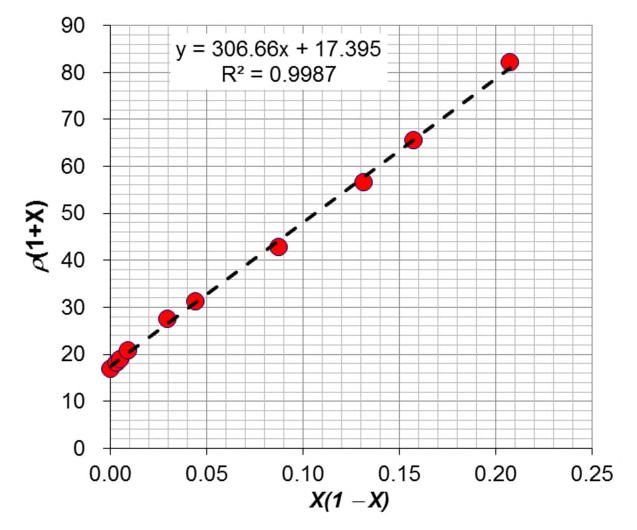
The above equation is of the straight line form y = mx +b, where m is the slope of the line. Therefore from the equation of the line y = 306.67x + 17.4, we have the effective Nordheim coefficient is Ceff = 306.67 nΩ m and ρ0 is 17.40 nΩ m.
If we calculate the resistivity using the values obtained above in the combined Nordheim-Mattheisen rule we obtain the following values in Table 2Q10-2
Table 2Q10-2: Ceff values calculated by fitting line to experimental data and by taking into account the effect of extra valence electron
Copyright © McGraw-Hill Education. All rights reserved. No reproduction or distribution without the prior written consent of McGraw-Hill Education.
For case I, the resistivity is calculated using an effective Nordheim coeffcieint (Ceff) and for the second case the combined Nordheim–Matthiessens rule is scaled up by (1 + X). It is observed that the values obtained by the later method is closer to the experimental results supporting the method of scaling taking into consideration the number of electrons donated by the solute atoms.
Comment: The Nordheim rule assumes that as the alloy composition changes, the number of conduction electrons per metal atom stays the same. In general, the resistivity due to the introduction of solute atoms (impurities) can be written as (see, for example, H. A. Fairbank, Phys. Rev. 66, 274, 1944; see p278.)
where Nat = atomic concentration (roughly constant) and n = average number of conduction electrons per atom. These two terms arise from the fact that scattering from the impurities involves something called the density of states g(EF) which depends on the electron concentration. n will depend on the valency of the solute atom. We can now plot
The plot of ρ vs. X(1 X)/(1+X)2/3 is shown in Figure 2Q10-3. The fit is comparable to the intuitive and classical modification of Nordheim's rule in Figure 2Q10-2.
Copyright © McGraw-Hill Education. All rights reserved. No reproduction or distribution without the prior written consent of McGraw-Hill Education.