Solution manual for optoelectronics and photonics principles and practices 2nd edition kasap 0132151 by lisa.jackson116

Preliminary Solutions to Problems and Question

Chapter 2

Note: Printing errors and corrections are indicated in dark red. Currently none reported.

2.1 Symmetric dielectric slab waveguide Consider two rays such as 1 and 2 interfering at point P in Figure 2.4 Both are moving with the same incidence angle but have different m wavectors just before point P. In addition, there is a phase difference between the two due to the different paths taken to reach point P. We can represent the two waves as E1(y,z,t) = Eocos(t mymz + ) and E2(y,z,t) = Eocos(t mymz)where the my terms have opposite signs indicating that the waves are traveling in opposite directions.  has been used to indicate that the waves have a phase difference and travel different optical paths to reach point P We also know that m =k1cosm and m = k1sinm, and obviously have the waveguide condition already incorporated into them through m Show that the superposition of E1 and E2 at P is given by

What do the two cosine terms represent?

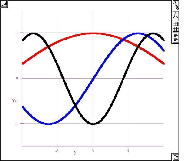
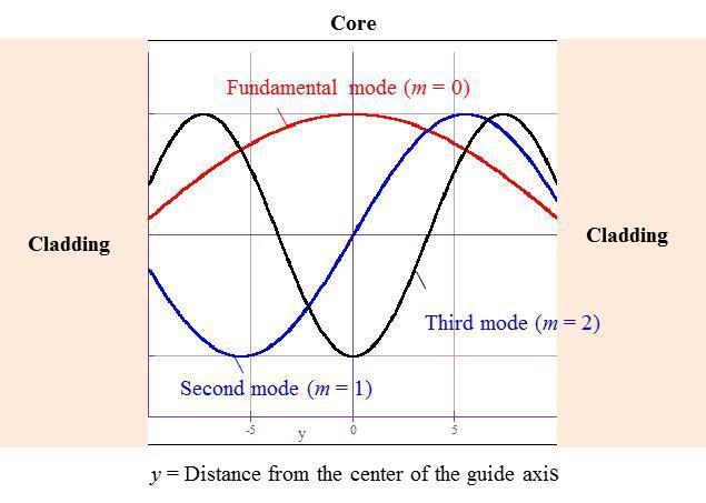
The planar waveguide is symmetric, which means that the intensity, E2 , must be either maximum (even m) or minimum (odd m) at the center of the guide. Choose suitable  values and plot the relative magnitude of the electric field across the guide for m = 0, 1 and 2 for the following symmetric dielectric planar guide : n1 = 1.4550, n2 = 1.4400, a = 10 m, = 1.5 m (free space), the first three modes have 1 = 88.84 , 2 = 87.673 = 86.51. Scale the field values so that the maximum field is unity for m = 0 at the center of the guide. (Note: Alternatively, you can choose  so that intensity (E2) is the same at the boundaries at y = a and y = a; it would give the same distribution.)

Use the appropriate trigonometric identity (see Appendix D) for cosA + cosB to express it as a product of cosines 2cos[(A+B)/2]cos[(A B)/2],

The first cosine term represents the field distribution along y and the second term is the propagation of the field long the waveguide in the z-direction. Thus, the amplitude is Amplitude =2E o

)

The intensity is maximum or minimum at the center. We can choose  = 0 ( m = 0),  =  ( m = 1),  = 2 ( m = 2), which would result in maximum or minimum intensity at the center. (In fact,  = m). The field distributions are shown in Figure 2Q1-1.

y, z,t)  2E o cos( m y 2  )cos(t m z  2  ) 1 1

Solution E(y)  E o cos(t  m z  m z   )  E o cos(t   m z m z)

E(y, z,t)  2E o cos( m y 1  )cos(t m z  2  )

cos( m y 2 

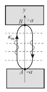
2.2 Standing waves inside the core of a symmetric slab waveguide Consider a symmetric planar dielectric waveguide. Allowed upward and downward traveling waves inside the core of the planar waveguide set-up a standing wave along y. The standing wave can only exist if the wave can be replicated after it has traveled along the y-direction over one round trip. Put differently, a wave starting at A in Figure 2.51 and traveling towards the upper face will travel along y, be reflected at B, travel down, become reflected again at A, and then it would be traveling in the same direction as it started. At this point, it must have an identical phase to its starting phase so that it can replicate itself and not destroy itself. Given that the wavevector along y is m, derive the waveguide condition.

Solution

From Figure 2.51 it can be seen that the optical path is

AB  BA  4a

With the ray under going a phase change with each reflection the total phase change is 

Figure 2Q1-1 Amplitudeof the electric field across the planar dielectric waveguide. Red, m = 0; blue, m = 1; black, m = 2. Figure 2.51 Upward and downward traveling waves along y set-up a standing wave. The condition for setting-up a standing wave is that the wave must be identical, able to replicate itself, after one round trip along y

 

a m 2

The wave will replicate itself, is the phase is same after the one round-trip, thus

as required.

2.3 Dielectric slab waveguide

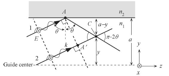
(a) Consider the two parallel rays 1 and 2 in Figure 2.52. Show that when they meet at C at a distance y above the guide center, the phase difference is

(b) Using the waveguide condition, show that

Hence find the amplitude of the field variation along y, across the guide. What is your conclusion?

Solution

(a) From the geometry we have the following: (a y)/AC = cos and C/AC =

)

The phase difference between the waves meeting at C is

  4a m 2  2m

 m  k1 cos m  2n1  cos m

2n1(2a) cos  m

m  m

and since

we get

m = k12(a y)cosm m

y  m   m (y)  m (m  m ) a

E( y)  Acos(t)  Acos[t   m ( y)]

Figure 2.52 Rays 1 and 2 are initially in phase as they belong to the same wavefront. Ray 1 experiences total internal reflection at A. 1 and 2 interfere at C There is a phase difference between the two waves.

 

cos(

2

 = kAC   kAC = k1AC k1ACcos( 2) 

where A is an arbitrary amplitude. Thus,

in which m/2, and cos(t +) is the time dependent part that represents the wave phenomenon, and the curly brackets contain the effective amplitude. Thus, the amplitude Eo is

To plot Eo as a function of y, we need to find m for m = 0, 1 , 2…The variation of the field is a truncated) cosine function with its maximum at the center of the guide. See Figure 2Q1-1.

2.4 TE field pattern in slab waveguide Consider two parallel rays 1 and 2 interfering in the guide as in Figure 2.52. Given the phase difference

between the waves at C, distance y above the guide center, find the electric field pattern E (y) in the guide. Recall that the field at C can be written as E( y)

. Plot the field

© 2013 Pearson Education, Inc., Upper Saddle River, NJ. All rights reserved. This publication is protected by Copyright and written permission should be obtained from the publisher prior to any prohibited reproduction, storage in a retrieval system, or transmission in any form or by any means, electronic, mechanical, photocopying, recording, or likewise. For information regarding permission(s), write to: Rights and Permissions Department, Pearson Education, Inc., Upper Saddle River, NJ 07458. Solutions Manual (Preliminary) 11 December 2012 Chapter 2 2.5 m  y  2 2 2 = k1AC[1 cos( 2)] k1AC[1 + cos(2)]  = k1(a y)/cos][ 1 + 2cos2 1]  = k1 (a y)/cos][2cos2]  = k1(a y)cos  (b) Given, 2(2a)n1  cos   m  m m  cos m  (mm )  mm 2n1(2a) k1(2a) mm Then,  m  2k1(a y)cos m m  2k1(a y) k1(2a) m    1 m  m  m  m a  y y (m  m ) a y  m  (y)  m (m  m )  m   m ( y)  m (m  m ) a a

E(y)  Acos(t)  Acos[t   m (y)]

E  2Acos[t  1  m (y)]cos1  m (y) or E  2Acos1  m (y)cos(t  ) = Eocos(t + )

E  2Acos m y (m   ) o 2 2a m

   (y)  m y (m   ) m m a m

 Acos(t)  Acos[t   m ( y)]

pattern for the first three modes taking a planar dielectric guide with a core thickness 20 m, n1 = 1.455 n2 = 1.440, light wavelength of 1.3 m.

The two waves interfering at C are out phase by ,

where A is an arbitrary amplitude. Thus,

in which

and

) is the time dependent part that represents the wave phenomenon, and the curly brackets contain the effective amplitude. Thus, the amplitude Eo is

To plot Eo as a function of y, we need to find m for m = 0, 1 and 2 , the first three modes. From Example 2.1.1 in the textbook, the waveguide condition is

we can now substitute for m which has different forms for TE and TM waves to find,

E(y)  Acos(t)  Acos[t   m (y)]

E  2Acos  t  1  (y) cos 1  (y) 2 m 2 m  1  or E  2Acos 2  m (y) cost   = Eocos(t + )   

m/2,

cos(



E  2Acos m y (m   ) o 2 2a m

t +

(2a)k1 cos m m  m

   1/2  sin2   n2    m    1   TE waves tan ak cos m   2    cos m  fTE ( m )

The above two equations can be solved graphically as in Example 2.1.1 to find m for each choice of m Alternatively one can use a computer program for finding the roots of a function. The above equations are functions of m only for each m. Using a = 10

= 1.3

m, n1 = 1.455 n2 = 1.440, the results are:

There is no significant difference between the TE and TM modes (the reason is that n1 and n2 are very close).

We can set A = 1 and plot Eo vs. y using

with the m and m values in the table above. This is shown in Figure 2Q4-1.

m, 



TE Modes m

m =

m = 2 m (degrees) 88.84   m (degrees) 163.75 147.02 129.69 TM Modes m = 0 m = 1 m = 2 m (degrees) 88.84   m (degrees) 164.08 147.66 130.60

= 0

Figure 2Q4-1 Field distribution across the core of a planar dielectric waveguide

E  2cos m y (m   ) o 2 2a m

2.5 TE and TM Modes in dielectric slab waveguide Consider a planar dielectric guide with a core thickness 20 m, n1 = 1.455 n2 = 1.440, light wavelength of 1.30 m. Given the waveguide condition, and the expressions for phase changes  and  in TIR for the TE and TM modes respectively,

using a graphical solution find the angle  for the fundamental TE and TM modes and compare their propagation constants along the guide. Solution

The waveguide condition is (2

we can now substitute for m which has different forms for TE and TM waves to find,

The above two equations can be solved graphically as in Example 2.1.1 to find m for each choice of m. Alternatively one can use a computer program for finding the roots of a function. The above equations are functions of m only for each m. Using a = 10 m,  = 1.3

m, n1 = 1.455 n2 = 1.440, the results are:

Education,

07458. Solutions Manual (Preliminary) 11 December 2012 Chapter 2 2.9 2 2 m 2 n  1 m 2 n  1 m 2  

Pearson

Inc., Upper Saddle River, NJ

   1/2    n 1/2   sin2   n2   sin2   2   m  n  m  n    1      1  tan1    and 2 m cos tan1 m    2  n   2  n cos m  1 

a)k



  m

1 cos

m m

   1/2  sin2   n2    m    1   TE waves tan ak cos m    2    cos m   1/2    fTE ( m ) sin2   n2    m    1   TM waves tan ak cos m    2    2  n   fTM ( m )  2   n1  cos m

TE Modes m = 0 m (degrees) 88.8361 m = k1sinm 7,030,883 m -1



TM Modes m = 0

m (degrees) 88.8340

m = k1sinm 7,030,878 m -1

Note that 5.24 m -1 and the -difference is only 7.510-5 %. The following intuitive calculation shows how the small difference between the TE and TM waves can lead to dispersion that is time spread in the arrival times of the TE and TM optical signals.

River,

Solutions Manual (Preliminary) 11

Chapter 2 2.10

Education, Inc., Upper Saddle

NJ 07458.

December 2012

Suppose that  is the delay time between the TE and TM waves over a length L. Then,

Over 1 km, the TE-TM wave dispersion is ~3.6 ps. One should be cautioned that we calculated dispersion using the phase velocity whereas we should have used the group velocity.

2.6 Group velocity We can calculate the group velocity of a given mode as a function of frequency

 using a convenient math software package. It is assumed that the math-software package can carry out symbolic algebra such as partial differentiation (the author used Livemath, , though others can also be used). The propagation constant of a given mode is

sin

where

and

imply

m and

m The objective is to express

and

in terms of

condition

Both  and  are now a function of  in Eqs (1) and (2). Then the group velocity is found by differentiating Eqs (1) and (2) with respect to  i.e.

where

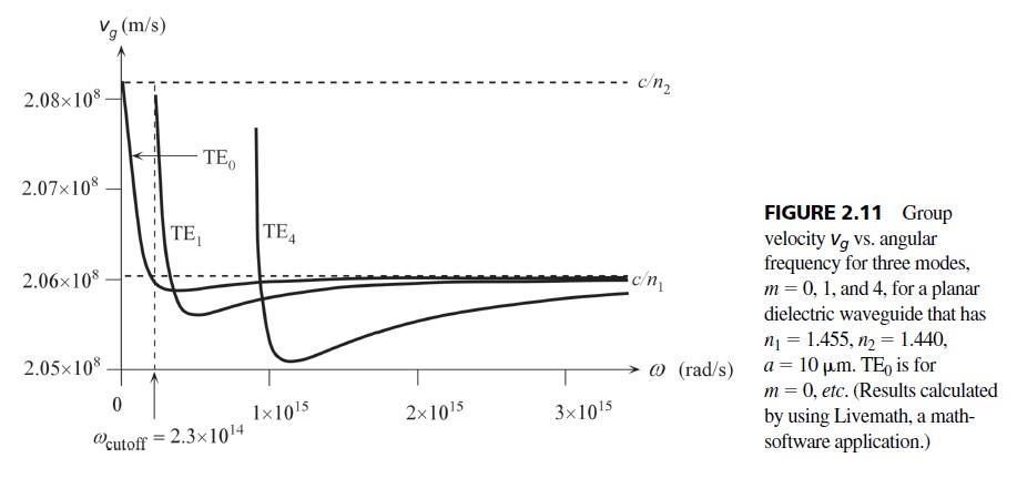
/d is found by differentiating the second term of Eq. (1). For a given m value, Eqs (2) and (3) can be plotted parametrically, that is, for each  value we can calculate  and vg and plot vg vs.  Figure 2.11 shows an example for a guide with the characteristics in the figure caption. Using a convenient math-software package, or by other means, obtain the same vg vs  behavior, discuss intermodal dispersion, and whether the Equation (2.2.2) is appropriate.

 1 1    (5.24m 1)   TE TM   L vTE vTM    (1.45 1015 rad/s) = 3.610-15 s m -1 = 0.0036 ps m -1

 = k1















 Since k1 = n1/c, the waveguide

is     sin2  (n / n )2 1/2 tan a  sin cos m   2  2 1 cos so that   tan arctansec sin2  (n / n )2  m( / 2) F ( ) (1) a 2 1 m where Fm() and a function of 

frequency  is given by   c  c F ( ) (2) n1 sin  n1 sin 

at a given

. The

 d  d    d   c  F m ( ) cos ( )  1  v g d d d  n  sin F  sin2  m    F ( )   1    m   c  F m ( )  i.e. v g  1 cot n sin F ( )  Group velocity, planar waveguide (3) 1  m  



Solution

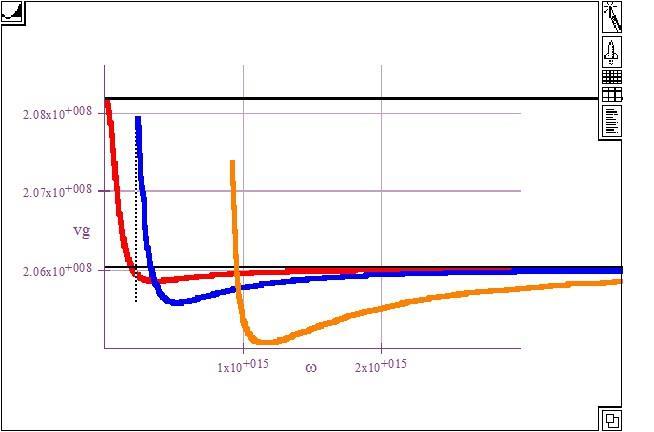
The results shown in Figure 2.11, and Figure 2Q6-1 were generated by the author using LiveMath based on Eqs (1) and (3). Obviously other math software packages can also be used. The important conclusion from Figure 2.11 is that although the maximum group velocity is c/n2, minimum group velocity is not c/n1 and can be lower. Equation (2.2.2) in §2.2 is based on using vgmax = c/n2 and vgmin = c/n1, that is, taking the group velocity as the phase velocity. Thus, it is only approximate.

2.7 Dielectric slab waveguide Consider a dielectric slab waveguide that has a thin GaAs layer of thickness 0.2 m between two AlGaAs layers. The refractive index of GaAs is 3.66 and that of the AlGaAs layers is 3.40. What is the cut-off wavelength beyond which only a single mode can propagate in the waveguide, assuming that the refractive index does not vary greatly with the wavelength? If a

Figure 2Q6-1 Group velocity vs. angular frequency  for three modes, TE0 (red), TE1 (blue) and TE4 (orange) in a planar dielectric waveguide. The horizontal black lines mark the phase velocity in the core (bottom line, c/n1) and in the cladding (top line, c/n1). (LiveMath used)

radiation of wavelength 870 nm (corresponding to bandgap radiation) is propagating in the GaAs layer, what is the penetration of the evanescent wave into the AlGaAs layers? What is the mode field width (MFW) of this radiation? Solution

Given n1 = 3.66 (AlGaAs), n2 = 3.4 (AlGaAs),

for only a single mode we need

The cut-off wavelength is 542 nm. When

= 870 nm,

Therefore,  = 870 nm is a single mode operation. For a rectangular waveguide, the fundamental mode has a mode field width

The decay constant  of the evanescent wave is given by,

The penetration depth

The penetration depth is half the core thickness. The width between two e -1 points on the field decays in the cladding is Width = 2a + 2× = 0.2 m + 2(0.102) m = 0.404 m.

2.8 Dielectric slab waveguide Consider a slab dielectric waveguide that has a core thickness (2a) of 20 m, n1 = 3.00, n2 = 1.50. Solution of the waveguide condition in Eq. (2.1.9) (in Example 2.1.1) gives the mode angles 0 and 1for the TE0 and TE1 modes for selected wavelengths as summarized in Table 2.7. For each wavelength calculate  and m and then plot  vs. m On the same plot show the lines with slopes c/n1 and c/n2. Compare your plot with the dispersion diagram in Figure 2.10

2a = 210-7 m or a

m,

V  2a (n 2 n 2 )1/2    1 2 2 2 2 1/2 2 2 1/2    2a(n1 n2 )  2(0.1 μm)(3.66 3.40 ) = 0.542 m.   2 2

= 0.1

2 (1 μm)(3.662 3.402 )1/2 V  (0.870 μm) = 0.979 < /2



2w  MFW  2a V  1  (0.2 μm) 0.979 1 = 0.404 m. o V 0.979

  V a  0.979 =9.79 (m)-1 or 9.79106 m -1 0.1 μm

 = 1/

[9.79 (m)-1] = 0.102 m.

= 1/

Table 2.7 The solution of the waveguide condition for a = 10 m, n1 = 3.00, n2 = 1.50 gives the incidence angles 0 and 

for modes 0 and 1 at the wavelengths shown.

Which is listed in Table 2Q8-1 in the second row under

constant along the guide, along z is given by Eq. (2.1.4) so that

which is the value listed in bold in Table 2Q8-1 for the

which is also listed in bold in Table 2Q8-1. We now have both

We can plot this 1 point for the m =0 mode at 0 = 7.15×105 m -1 along the x-axis, taken as the -axis, and  = 2.54×1013 s -1 along the y-axis, taken as the -axis, as shown in Figure 2Q8-1. We can also plot the 1 point we have for the m = 1 mode.

Propagation constants () at other wavelengths and hence frequencies () can be similarly calculated. The results are listed in Table 2Q8-1 and plotted in Figure 2Q8-1. This is the dispersion diagram. For comparison the dispersion  vs  for the core and the cladding are also shown. They are drawn so that the slope is c/n1 for the core and c/n2 for the cladding.

Thus, the solutions of the waveguide condition as in Example 2.1.1 generates the data in Table 2Q8-1 for 2a = 10 m, n1 = 3; n2 = 1.5.

Manual (Preliminary) 11 December

Chapter 2 2.14

Solutions

2012

 m 15 20 25 30 40 45 50 70 100 150 200 0  77 8 74 52 71 5 68 7 63 9 61 7 59 74 53 2 46 4 39 9 36 45 1  65.2 58.15 51.6 45.5 35.5 32.02 30.17 ‐ ‐ ‐ ‐Solution

25 m

25×10-6 m. The free space propagation

k = 2/ = 225×10-6 m = 2.513×105 m -1 . The propagation constant within the core is k1 = n1k = (3.00)( 2.513×105 m -1) = 7.540×105 m -1 The angular frequency  = ck = (3×108 m s -1)( 2.513×105 m -1) = 7.54×1013 s -1 .



m.

propagation

m

k1sinm or 0 = k1sin0 = (7.540×105 m -1)sin(71.5) = 7.540×105 m -1 = 7.15×105 m -1 .

Consider the case example for =

constant

= 25

The

m = 0

 =

m. Similarly 1 = k1sin1 = (7.540×105 m -1)sin(51 6) = 7.540×105 m -1 = 5.91×105 m -1

mode at

 1 at  = 2.54×1013 s -1



and

(2a) of 20 m, n1 = 3.00, n2 = 1 50.  m 15 20 25 30 40 45 50 70 100 150 200  1013 s ‐1 12 6 9.43 7.54 6.283 4.71 4.19 3.77 2.69 1.89 1.26 0.94 0  77 8 74 52 71.5 68 7 63 9 61 7 59 74 53 2 46 4 39 9 36 45 1  65 2 58 15 51.6 45 5 35 5 32 02 30 17 ‐ ‐ ‐ ‐

Table2Q8-1 Planar dielectric waveguide with a core thickness

Figure 2Q8-1 Dispersiondiagram for a planar dielectric waveguidethat has a core thickness (2a) of 20 m, n1 = 3.00, n2 = 1.50. Black, TE0 mode. Purple: TE1 mode. Blue: Propagation along the cladding. Red: Propagation along the core

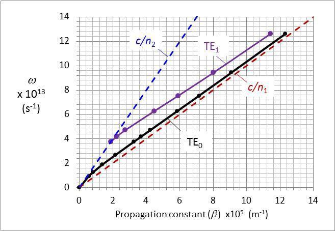
Author's Note: Remember that the slope at a particular frequency  is the group velocity at that frequency. As apparent, for the TE0 (m = 0) mode, this slope is initially (very long wavelengths) along the blue curve at low frequencies but then along the red curve at high frequencies (very short wavelengths). The group velocity changes from c/n2 to c/n1

2.9 Dielectric slab waveguide Dielectric slab waveguide Consider a planar dielectric waveguide with a core thickness 10 m, n1 = 1.4446, n2 = 1.4440. Calculate the V-number, the mode angle m for m = 0 (use a graphical solution, if necessary), penetration depth, and mode field width, MFW = 2a + 2, for light wavelengths of 1.0 m and 1.5 m. What is your conclusion? Compare your MFW calculation with 2wo = 2a(V+1)/V The mode angle 0, is given as 0 = 88.85 for  = 1 m and 0 = 88.72 for  = 1.5 m for the fundamental mode m = 0.

Solution

 = 1 m, n1 = 1.4446, n2 = 1.4440, a = 5 m. Apply

to obtain V = 1.3079

V  2a n 2 n 2 1/2  1 2

Solve the waveguide condition

graphically as in Example 2.1.1 to find:

to calculate the penetration depth:

= 5.33 

 MFW = 2a + 2 = 20.65 m

We can also calculate MFW from MFW = 2a(V+1)/V = 2(5 m)(1.3079+1)/(1.3079) = 17.6 m (Difference = 15%)

 = 1.5 m, V = 0.872, single mode. Solve waveguide condition graphically that the mode angle is o = 88.72 .

 = 1/ = 9.08 m.

 MFW = 2a + 2 = 28.15 m.

Compare with MFW = 2a(V+1)/V = 2(5 m)(0.872+1)/(0.872) = 21.5 m (Difference = 24%)

Notice that the MFW from 2a(V+1)/V gets worse as V decreases. The reason for using MFW = 2a(V+1)/V, is that this equation provides a single step calculation of MFW. The calculation of the penetration depth  requires the calculation of the incidence angle  and 

Author's Note: Consider a more extreme case

 = 5 m, V = 0.262, single mode. Solve waveguide condition graphically to find that the mode angle is o = 88.40

 = 1/ = 77.22 m.

 MFW = 2a + 2 = 164.4 m.

Compare with MFW = 2a(V+1)/V = 2(5 m)(0.262 + 1)/(0.262) = 48.2 m (Very large difference.)

 1/2    sin2   n2    m    1   tan ak cos m    2    cos m  f ( m )

c = 88.35

the

(for m = 0) is o = 88.85 .

 n 2 1/2  2n2  1  sin2  1 1  m   m   n2    

and

mode angle

Then use

 =



2.10 A multimode fiber Consider a multimode fiber with a core diameter of 100 m, core refractive index of 1.4750, and a cladding refractive index of 1.4550 both at 850 nm. Consider operating this fiber at  = 850 nm. (a) Calculate the V-number for the fiber and estimate the number of modes. (b) Calculate

the wavelength beyond which the fiber becomes single mode. (c) Calculate the numerical aperture. (d)

Calculate the maximum acceptance angle. (e) Calculate the modal dispersion  and hence the bit rate  distance product.

For wavelengths longer than 31.6 m, the fiber is a single mode waveguide. The numerical aperture NA is

If max is the maximum acceptance angle, then,

Given that

, maximum bit-rate is

i.e. BL = 13 Mb s-1 km (only an estimate)

We neglected material dispersion at this wavelength which would further decrease BL. Material dispersion and modal dispersion must be combined by

Manual (Preliminary) 11 December

Chapter 2 2.18 2

Solutions

2012

Solution

n2 = 1.455, 2a = 10010-6 m or a = 50 m and = 0.850 m. The V-number

2 2 1/2 V  2a n 2 n 2 1/2  2π(50 μm)(1.475 1.455 ) = 89.47  1 2 Number of modes M, (0.850 μm) M  V  2 89.472 2  4002

V  2a n 2 n 2 1/2  2.405  1 2 2an 2 n 2 1/2 2(50 μm)(1.4752 1.4552 )1/2 or   1 2  2.405 2.405 = 31.6 m

Given

= 1.475,

is,

The fiber becomes monomode when,

2 2 1/2 2 2 1/2 NA  (n1 n2 )  (1.475 1.455 ) = 0.242

 NA  max  arcsin  n o

  arcsin(0.242/1) = 14  intermode  n1 n2  1.475 1.455 L c 3108 ms -1 = 66.7 ps m -1 or 67.6 ns per km

 



BL  0.25L  0.25L  0.25  total  intermode (0.29)(66.7ns km-1)

Modal dispersion is given by

0.29

For example, assuming an LED with a spectral rms deviation  of about 20 nm, and a Dm 200 ps km-1 nm -1 (at about 850 nm)we would find the material dispersion as

material = (200 ps km-1 nm -1)(20 nm)(1 km)  4000 ps km-1 or 4 ns km-1 , which is substantially smaller than the intermode dispersion and can be neglected.

2.11 A water jet guiding light One of the early demonstrations of the way in which light can be guided along a higher refractive index medium by total internal reflection involved illuminating the starting point of a water jet as it comes out from a water tank. The refractive index of water is 1.330. Consider a water jet of diameter 3 mm that is illuminated by green light of wavelength 560 nm. What is the V-number, numerical aperture, total acceptance angle of the jet? How many modes are there? What is the cut-off wavelength? The diameter of the jet increases (slowly) as the jet flows away from the original spout. However, the light is still guided. Why?

Light guided along a thin water jet. A small hole is made in a plastic soda drink bottle full of water to generate a thin water jet. When the hole is illuminated with a laser beam (from a green laser pointer), the light is guided by total internal reflections along the jet to the tray Water with air bubbles (produced by shaking the bottle) was used to increase the visibility of light. Air bubbles scatter light and make the guided light visible. First such demonstration has been attributed to JeanDaniel Colladon, a Swiss scientist, who demonstrated a water jet guiding light in 1841.

Total acceptance angle, assuming that the laser light is launched within the water medium

Modes = M = V2/2 = (15104)2/2 = 1.14×108 modes (~100 thousand modes)

The curoff wavelength corresponds to V = 2.405,

The large difference in refractive indices between the water and the air ensures that total internal reflection occurs even as the width of the jet increases, which changes the angle of incidence.

2.12 Single mode fiber Consider a fiber with a 86.5%SiO2-13.5%GeO2 core of diameter of 8 m and refractive index of 1.468 and a cladding refractive index of 1.464 both refractive indices at 1300 nm

Solution V-number 2 1/2 -3 -9 2 2 1/2 V = (2a/)(n1 2 n2 ) Numerical aperture = (2×1.5×10 /550×10 )(1.330 1.000 ) = 15104 NA= (n1 2  n2 2)1/2 = (1.3302 1.0002)1/2 = 0.8814

sinmax = NA/n0





= 0.113/1.33 or

max = 41.4°. Total acceptance 2o = 82.8

V = (2a/)NA =

c = [2aNA]/2.405 = [(2)(4 m)(0.8814)]/2.405 = 3.5

that is

2.405

where the fiber is to be operated using a laser source with a half maximum width of 2 nm. (a) Calculate the V-number for the fiber. Is this a single mode fiber? (b) Calculate the wavelength below which the fiber becomes multimode. (c)Calculate the numerical aperture. (d) Calculate the maximum acceptance angle. (e) Obtain the material dispersion and waveguide dispersion and hence estimate the bit rate

distance product (B

L) of the fiber.

(b) Since V < 2.405, this is a single mode fiber. The fiber becomes multimode when

For wavelengths shorter than 1.13 m, the fiber is a multi-mode waveguide.

(d) If max is the maximum acceptance angle, then,

so that the total acceptance angle is 12.4

. (e) At

Obviously material dispersion is 15 ps km-1 and waveguide dispersion is 10 ps km-1

The maximum bit-rate distance product is then



Solution (a) Given n1 = 1.475, n2 = 1.455, 2a = 810-6 m or a = 4 m and =1.3 m. The V-number is, 2 2 1/2 V  2a n 2 n 2 1/2  2(4 μm)(1.468 1.464 ) = 2.094  1 2 (1.3 μm)



V  2a (n 2 n 2 )1/2  2.405  1 2 2an 2 n 2 1/2 2(4 μm)1.4682 1.4642 1/2 or   1 2  2 405 2.405 =1.13 m

 2 2 1/2 2 2 1/2 NA  n1 n2  (1 468 1 464 ) = 0.108

 NA  max  arcsin  n o   arcsin(0.108/1)= 6.2 





m,

,

2.22, Dm  7.5 ps km-1 nm -1 , Dw  5 ps km-1 nm -1 . 1/2  L D m  D w 1/2 = | 7.5 5 ps km-1 nm -1|(2 nm) = 15 ps km-1 + 10 ps km-1 =

ns km

=1.3

from

vs.

Figure

0.025

-1

BL  0.59L  0.59 =

Gb s-1 km. 1/2 0.025 ns km

23.6

2.13 Single mode fiber Consider a step-index fiber with a core of diameter of 9 m and refractive index of 1.4510 at 1550 nm and a normalized refractive index difference of 0.25% where the fiber is to be operated using a laser source with a half-maximum width of 3 nm. At 1.55 m, the material and

waveguide dispersion coefficients of this fiber are approximately given by Dm = 15 ps km-1 nm -1 and Dw = 5 ps km-1 nm -1 (a) Calculate the V-number for the fiber. Is this a single mode fiber? (b) Calculate the wavelength below which the fiber becomes multimode. (c) Calculate the numerical aperture. (d) Calculate the maximum total acceptance angle. (e) Calculate the material, waveguide and chromatic dispersion per kilometer of fiber. (f) Estimate the bit rate

distance product (BL) of this fiber. (g) What is the maximum allowed diameter that maintains operation in single mode? (h) What is the mode field diameter?

(a) The normalized refractive index difference  and n1 are given.

(b) For multimode operation we need

(d) If max is the maximum acceptance angle, then,

(f) Maximum bit-rate would be



Solution

Apply,  = (n1n2)/n1 = (1.451 n2)/1.451 = 0.0025, and solving for n2 we find n2 = 1.4474. The V-number is given by 2 2 1/2 V  2a (n 2 n 2 )1/2  2(4.5 μm)(1.4510 1.4474 ) = 1.87; single mode fiber.  1 2 (1.55 μm)

2 2 1/2 2a ( 2 2 )1/ 2 2(4.5 μm)(1.4510 1.4474 ) 2.405 V   n1 n2      < 1.205 m.

2 2 1/2 2 2 1/2 NA  (n1 n2 )  (1.4510 1.4474 ) = 0.1025.

 NA  max  arcsin  n o 

arcsin(0.1025/1)

  Total

2amax is 11.8  . (e)

5 ps km-1 nm -1 and Dm =  ps km-1 nm -1 . Laser diode

(FWHM) 1/2 = 3 nm Material dispersion 1/2/L = |Dm|1/2 = (15 ps km-1 nm -1)(3 nm) = 45 ps km-1 Waveguide dispersion 1/2/L = |Dw|1/2 = ( 5 ps km-1 nm -1)(3 nm) = 5 ps km-1 Chromatic dispersion, 1/2/L = |Dch|1/2 = ( 5 ps km-1 nm -1 + 15 ps km-1 nm -1)(3 nm) =

ps km-1

= 5.89

acceptance angle

Given,

spectral width

i.e. BL  20 Mb s-1 km (only an estimate)

(g) To find the maximum diameter for SM operation solve,

2.14 Normalized propagation constant b Consider a weakly guiding step index fiber in which (

) /

1 is very small. Show that

can be assumed were convenient. The first equation can be rearranged as

Note: Since  is very small,

where x is small. Taylor's expansion in x to the first linear term would then provide a linear relationship between  and b.

Taylor expansion around x

0 and truncating the expression, keeping only the linear term yields,

then using the assumption

we get

2 2 1/2 V  2a ( 2  1 n 2 )1/2  2(a μm)(1.4510 1.4474 ) (1.55 μm)  2.405  2a = 11.5 m.

2w  2a(0.65  1.619V 3/2  2.879V 6 )= 12.2 m

(h) The mode filed diameter 2w is

( / k)2 n 2 ( / k) n b  2  2 n 2 n 2 n n 1 2 1 2

n1 

2 2 2 1/2 2 1/2 2 2 2  / k  [n2  b(n1 n2 )]  n2 (1 x) ; x  b(n1 n2 )/ n2

Solution 1 1  2 2 2 2 2 k  [n2  b(n1  n 2 n2 )]   n2 (1  x) where x  b 1 1  n2 

 nx  x   b  n 2  b k  n2  2  n2 1  2  n2 1  2  n 2 1  n2  n 2 n 2     2    2   n2 

n1 



2.15 Group velocity of the fundamental mode Reconsider Example 2.3.4, which has a single mode fiber with core and cladding indices of 1.4480 and 1.4400, core radius of 3 m, operating at 1.5 m. Use the equation

to recalculate the propagation constant  Change the operating wavelength to  by a small amount, say 0.01%, and then recalculate the new propagation constant . Then determine the group velocity vg of the fundamental mode at 1.5 m, and the group delay g over 1 km of fiber. How do your results compare with the findings in Example 2.3.4?

From example 2.3.4, we have

vs.  for pure SiO2 and SiO2-13.5 mol.%GeO2 in Table1.2 in Ch. 1. The refractive index increases linearly with the addition

A single mode fiber design The Sellmeier dispersion equation provides

b  (/ k) n2 ;  = n k[1 + b] n1 n2

Solution

b  0.3860859, k  4188790m 1 ,   2c  1.2566371015 s 1    n k[1 b]  (1.4400)(4188790m 1)  (0.3860859) (1.4480 1.4400)  2   6044795m 1 1.4480   1.5μm(1 1.001)  1.5015μm , b  0 3854382, k  4184606m 1 ,   1.255382 1015 s 1    n k[1 b]  (1.4400)(418406m 1)  (0.3854382) (1.4480 1.4400)  2    6038736m 1 Group Velocity 1.4800 15 1      (1.255382 1.256637)10 s  2.0713108 ms 1 g    (6.038736 6.044795)106 m 1  g  4.83μsover 1 km. Comparing to Example 2.3.4 2.0713 2.0706 %diff  2.0706 100%  0.03% 2.16

of GeO2 to SiO2 from 0 to 13.5 mol.%. A single mode step index fiber is required to have the following properties: NA = 0.10, core diameter of 9 m, and a cladding of pure silica, and operate at 1.3 m. What should the core composition be?

Solution

The Sellmeier equation is

From Table1.2 in Ch.1. Sellmeier coefficients as as follows

Therefore, for  = 1.3 m pure silica has n(0) = 1.4473 and SiO2-13.5 mol.%GeO

Confirming that for NA=0.10 we have a single mode fiber

has

, assuming a linear relationship, can be written as

2.17 Material dispersion If Ng1 is the group refractive index of the core material of a step fiber, then the propagation time (group delay time) of the fundamental mode is

Since Ng will depend on the wavelength, show that the material dispersion coefficient Dm is given approximately by

Using the Sellmeier equation and the constants in Table 1.2 in Ch. 1, evaluate the material dispersion at= 1.55 m for pure silica (SiO2) and SiO2-13.5%GeO2 glass. Solution

From Ch. 1 we know that

Manual (Preliminary) 11 December

Chapter 2 2.27 1 2 3

Solutions

2012

A 2 A 2 A 2 n 2  1  1  2  3 2 2 2 2 2 2

Sellmeier A1 A2 A3 1 m 2 m 3 m SiO2 (fused silica) 0.696749 0.408218 0.890815 0.0690660 0.115662 9.900559 86.5%SiO2‐13.5%GeO2 0.711040 0.451885 0.704048 0.0642700 0.129408 9.425478

n(13.5)= 1.4682

n 2  2a NA  2(4.5μm)(0.1)= 2.175  (1.3μm) Apply NA  n 2 n 2 1/2 to obtain n  NA2  n 2 1/2 =(0.12+1.44732)1/2 = 1.4508 1 2 1 2 The refractive index n(x) of SiO2-x mol.%GeO2

n(x)  n(0)1 x   n(13.5) x    13.5  13.5

n(x) = n1 = 1.4508

x = 2.26

Substituting

gives

  L / v g  LNg1 / c

d D m   d 2 n  Ld c d2

Differentiate

with respect to wavelength  using the above relationship between Ng and n.

From Ch. 1 we know that the Sellmeier equation is

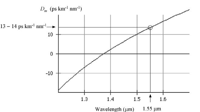
We can use the Sellmeier coefficient in Table1.2 in Ch.1 to find n vs. , dn/d and d2n/d , and, from Eq. (1), Dm vs as in Figure 2Q17-1. At  = 1.55 m, Dm =

  L  LNg1 v g c  d  L dNg1 L  dn    d n dn    L  d n d c d d c  d  d 2 n d2 d  c d2 Thus, D m  Ld  c d2 (1)



A 2 A 2 A 2 n 2 1  1  2  3 (2) 2 2 2 2 2 2 The Sellmeier

The 1, 2, 3 are in m. A1 A2 A3 1 2 3 SiO2‐13.5%GeO2 0.711040 0.451885 0.704048 0.0642700 0.129408 9.425478

coefficients for SiO2-13.5%GeO2.

-1

14 ps km

Figure 2Q17-1 Materials dispersion Dm vs. wavelength (LiveMath used). (Other math programs such as Matlab can also be used.)

2.18 Waveguide dispersion Waveguide dispersion arises as a result of the dependence of the propagation constant on the V-number, which depends on the wavelength. It is present even when the refractive index is constant; no material dispersion. Let us suppose that n1 and n2 are wavelength (or k) independent. Suppose that  is the propagation constant of mode lm and k = 2π/in which is the free space wavelength. Then the normalized propagation constant b and propagation constant are related by

The group velocity is defined and given by

Show that the propagation time, or the group delay time,

of the mode is

Show that

and that the waveguide dispersion coefficient is

Show that,

which simplifies to

 = n

(1)

2k[1 + b]

v  d  c dk g d d



  L  Ln2  Ln2 d(kb) (2) v g c Given the definition of V, c dk and V  ka[n 2 n 2]1/2  kan (2)1/2 (3) d(Vb)  d bkan (2)1/ 2  an (2)1/ 2 d (bk) (4)

dV dV 2 2 dV d Ln  d 2 (Vb)  2 V (5) d c dV 2

D  d n  d 2 (Vb)  2 V (6) w Ld c dV 2

Figure 2.53 shows the dependence of V[d2(Vb)/dV2] on the V-number. In the range 1.5 < V < 2.4,

d 2 (Vb) V  dV 2 1.984 V 2 D  n2 1.984  (n1 n2 ) 1.984 (7)

w c V 2 c V 2

Consider a fiber with a core of diameter of 8 m and refractive index of 1.468 and a cladding refractive index of 1.464, both refractive indices at 1300 nm. Suppose that a 1.3 m laser diode with a spectral linewidth of 2 nm is used to provide the input light pulses. Estimate the waveguide dispersion per kilometer of fiber using Eqs. (6) and (8).

Solution

Waveguide dispersion arises as a result of the dependence of the propagation constant on the V-number which depends on the wavelength. It is present even when the refractive index is constant; no material dispersion. Let us suppose that n1 and n2 are wavelength (or k) independent. Suppose that  is the propagation constant of mode lm and k = 2/where is the free space wavelength. Then the normalized propagation constant b is defined as,

Show that for small normalized index difference  = (n1 n2)/n1, Eq. (1) approximates to

which gives  as,

] (3)

The group velocity is defined and given by

Thus, the propagation time  of the mode is

1 5 1 V[d2(Vb)/dV2] 0 5 0 0 1 2 3 V-number

Figure 2.53 d2(Vb)/dV2 vs V-number for a step index fiber. (Data extracted from W A. Gambling et al. The Radio and Electronics Engineer, 51, 313, 1981.)

( / k)2 n 2 b  2 n 2 n 2 (1) 1 2

b  (/ k) n2 n1 n2 (2)



= n2k[1 + b

v  d  c dk g d d

where we assumed 

constant (does not depend on the wavelength). Given the definition of V,

This means that  depends on V as,

Dispersion, that is, spread  in due to a spread  can be found by differentiating Eq. (6) to obtain,

The waveguide dispersion coefficient is defined as

Figure 2.53 shows the dependence of V[

In the range 2 < V < 2.4,

so that Eq. (8) becomes,

V  ka[n 2 n 2 ]1/2  ka[(n  n )(n n )]1/2 1 2 1 2 1 2 1/2   n n   ka (n  n )n  1 2  (5)  1 2 1    n1   ka[2n n ]1/2  kan (2)1/2 From Eq. (5), 2 1 2 d(Vb)  d bkan (2)1/ 2  an (2)1/ 2 d (bk) dV dV 2 2 dV



  Ln2  Ln2 d(Vb) (6) c c dV

d Ln  dV d d(Vb) Ln   V  d 2 (Vb)  2  2   d c d dV dV c    dV 2 (7)  Ln2 V c d 2 (Vb) dV 2

D  d n  d 2 (Vb)  2 V (8) w Ld c dV 2

d 2 (Vb) V  dV 2

1.984 V 2 D  n2 1.984  (n1 n2 ) 1.984 (9) w c V 2 c V 2

d (Vb)/dV ] on the V-number.

Equation (6) should really have Ng2 instead of n2 in which case Eq. (10) would be

Consider a fiber with a core of diameter of 8 m and refractive index of 1.468 and a cladding refractive index of 1.464 both refractive indices at 1300 nm. Suppose that a1.3 m laser diode with a spectral linewidth of 2 nm is used to provide the input light pulses. Estimate the waveguide dispersion per kilometer of fiber using Eqs. (8) and (11).

2.19 Profile dispersion Total dispersion in a single mode, step index fiber is primarily due to material dispersion and waveguide dispersion. However, there is an additional dispersion mechanism called profile dispersion that arises from the propagation constant of the fundamental mode also depending on the refractive index difference . Consider a light source with a range of wavelengths  coupled into a step index fiber. We can view this as a change in the input wavelength. Suppose that n1, n 2, hence depends on the wavelength  The propagation time, or the group delay time, g per unit length is

where k is the free space propagation constant (2/),and we used dcdk. Since  depends on n1,  and V, consider g as a function of n1,  (thus n2), and V. A change in  will change each of these quantities. Using the partial differential chain rule,

1.984N D  g 2  w c(2a)2 2n 2 (11)

2 2 1/2 V  2a n 2 n 2 1/2  2(4 μm)(1.468 1.464 ) = 2.094  1 2 (1.3 μm) and  = (n1 n2)/n1 = (1.468 1.464)/1.468 = 0.00273. From the graph, Vd2(Vb)/dV2 = 0.45, 2 3 D  n2 V d (Vb)  (1.464)(2.7310 ) (0.45) w c dV 2 (3108 ms -1)(1300 10 9 m)  Dw  4.610-6 s m -2 or 4.6 ps km-1 nm -1 Using Eq. (10) D w  1.984 c(2a)2 2n   1.984(1300 10 9 m) (3 108 ms -1)[2  4 10 6 m]2 2(1.464)]  Dw  4.610-6 s m -2 or 4.6 ps km-1 nm -1 For 1/2 = 2 nm we have, 1/2 = |Dw|L 1/2 = (4.6 ps km-1 nm -1)(2 nm) = 9.2 ps/km

 g  1/vg  d / d  (1/ c)(d / dk) (1)

The mathematics turns out to be complicated but the statement in Eq. (2) is equivalent to

Total dispersion = Material dispersion (due to ∂n1/∂)

+ Waveguide dispersion (due to ∂V/∂)

+ Profile dispersion (due to ∂/∂) in which the last term is due to  depending on; although small, this is not zero. Even the statement in Eq. (2) above is over simplified but nonetheless provides an insight into the problem. The total intramode (chromatic) dispersion coefficient Dch is then given by

Dch = Dm + Dw + Dp (3) in which Dm, Dw, Dp are material, waveguide, and profile dispersion coefficients respectively. The waveguide dispersion is given by Eq. (8) and (9) in Question 2.18, and the profile dispersion coefficient is (very) approximately1 ,

in which b is the normalized propagation constant and Vd

vs. V is shown in Figure 2.53,we can also use

Consider a fiber with a core of diameter of 8 m. The refractive and group indices of the core and cladding at  = 1.55 m are n1 = 1.4500, n 2 = 1.4444, Ng1 = 1.4680, Ng 2 = 1.4628, and d/d = 232 m -1 . Estimate the waveguide and profile dispersion per km of fiber per nm of input light linewidth at this wavelength. (Note: The values given are approximate and for a fiber with silica cladding and 3.6% germania-doped core.)

Solution

Total dispersion in a single mode step index fiber is primarily due to material dispersion and waveguide dispersion. However, there is an additional dispersion mechanism called profile dispersion that arises from the propagation constant  of the fundamental mode also depending on the refractive index difference . Consider a light source with a range of wavelengths  coupled into a step index fiber. We can view this as a change in the input wavelength. Suppose that n1, n 2, hence depends on the wavelength  The propagation time, or the group delay time, g per unit length is

Since  depends on n1,  and V, let us consider g as a function of n1,  (thus n2) and V. A change in will change each of these quantities. Using the partial differential chain rule, 1 J. Gowar, Optical Communication Systems, 2nd Edition (Prentice Hall, 1993). Ch 8 has the derivation of this equation

D Ng1  V d (Vb)  d  p   c dV 2   d (4)   

2(Vb)/dV2

Vd2(Vb)/dV2  1.984/V2

1 1  d   g     (1) vg c  dk 

The mathematics turns out to be complicated but the statement in Eq. (2) is equivalent to

Total dispersion = Materials dispersion (due to n1/)

+ Waveguide dispersion (due to V/)

+ Profile dispersion (due to /)

where the last term is due  depending on; although small this is not zero. Even the above statement in Eq. (2) is over simplified but nonetheless provides an sight into the problem. The total intramode (chromatic) dispersion coefficient Dch is then given by

Dch = Dm + Dw + Dp (3)

where Dm, Dw, Dp are material, waveguide and profile dispersion coefficients respectively. The waveguide dispersion is given by Eq. (8) in Question 2.6 and the profile dispersion coefficient away is (very) approximately,

Consider

are

From the graph in Figure 2.53, when

D Ng1  V d (Vb)  d  p   c dV 2   d (4)   

and Vd2(Vb)/dV2 vs. V is shown in Figure 2.53. The term Vd2(Vb)/dV2  1.984/V2

where b is the normalized propagation constant

8 m.

and

core and cladding

1.55 

1.4504, n 2 = 1.4450, Ng1 = 1.4676, Ng 2 = 1.4625. d/d = 161 m -1 . 2 2 1/2 V  2a n 2 n 2 1/2  2(4 μm)(1.4504 1.4450 ) = 2.03  1 2 (1.55 μm) and  = (n1 n2)/n1 = (1.4504-1.4450)/1.4504 = 0.00372

a fiber with a core of diameter of

The refractive

group indexes of the

at  =

2.03, Vd2(Vb)/dV2  0.50,

dispersion: N  d 2 Vb  d  D  g1 V ( )    1.4676 0.50161m 1 c  dV 2  d  3108 ms 1  Dp = 3.8 10-7 s m -1 m -1 or 0.38 ps km-1 nm -1 Waveguide dispersion: D w  1.984 c(2a)2 2n   1.984(1500 10 9 m) (3 108 ms -1)[2  4 10 6 m]2 2(1.4450)]  Dw  5.6 ps km-1 nm -1

Profile

Profile dispersion is more than 10 times smaller than waveguide dispersion.

2.20 Dispersion at zero dispersion coefficient

Since the spread in the group delay  along a fiber depends on the , the linewidth of the source we can expand  as a Taylor series in . Consider the expansion at  = 0 where Dch = 0. The first term with  would have d /d as a coefficient that is Dch, and at 0 this will be zero; but not the second term with ( that has a differential, d2/d or dDch/d. Thus, the dispersion at 0 would be controlled by the slope S0 of Dch vs.  curve at 0. Show that the chromatic dispersion at 0 is

A single mode fiber has a zero-dispersion at 0 = 1310 nm, dispersion slope S0 = 0.090 ps nm2 km. What is the dispersion for a laser with  = 1.5 nm? What would control the dispersion?

Solution

Consider the Taylor expansion for , a function of wavelength, about its center around, say at 0, when we change the wavelength by For convenience we can the absolute value of  at 0 as zero since we are only interested in the spread . Then, Taylor's expansion gives,

This can be further reduced by using a narrower laser line width since depends on (

2.21 Polarization mode dispersion (PMD) A fiber manufacturer specifies a maximum value of 0.05 ps km-1/2 for the polarization mode dispersion (PMD) in its single mode fiber. What would be the dispersion, maximum bit rate and the optical bandwidth for this fiber over an optical link that is 200 km long if the only dispersion mechanism was PMD?



  L 2 S0 () 2

  f ()  d ()  1 d 2 ()2   d d 2 2! d2 d  d  d    0  1  ()2  0  1   ()2  1 D ()2 2! d2 2! dt  d  2! dt ch  L 2 1 km  -2 -1 2   S0 ()  2 2 0.090psnm km 2nm = 1.01 ps



Solution Dispersion   DPMDL1/2  0.05ps km 1/2 (200km)1/2  0.707ps Bit rate B  0.59  0.59  8.35Gbs -1  0.707ps Optical bandwidth fop  0.75B  (0.75)(8.35Gbs 1)  6.26GHz

2.22 Polarization mode dispersion Consider a particular single mode fiber (ITU-T G.652 compliant) that has a chromatic dispersion of 15 ps nm-1 km-1 . The chromatic dispersion is zero at 1315 nm, and the dispersion slope is 0.092 ps nm-2 km-1 The PMD coefficient is 0.05 ps km-1/2 Calculate the total dispersion over 100 km if the fiber is operated at 1315 nm and the source is a laser diode with a linewidth (FWHM)  = 1 nm What should be the linewidth of the laser source so that over 100 km, the chromatic dispersion is the same as PMD?

We need the chromatic dispersion at 0, where the chromatic dispersion Dch = 0. For L = 100 km, the chromatic dispersion is

The rms dispersion is

2.23 Dispersion compensation Calculate the total dispersion and the overall net dispersion

coefficient when a 900 km transmission fiber with Dch = +15 ps nm -1 km-1 is spliced to a compensating fiber that is 100 km long and has Dch = 110 ps nm-1 km-1 What is the overall effective dispersion coefficient of this combined fiber system? Assume that the input light spectral width is 1 nm.

Solution

Using Eq. (2.6.1) with  = 1 nm, we can find the total dispersion

)(900

+ ( 110 ps nm-1 km-1)(100 km)](1 nm) = 2,500 ps nm-1 for 1000 km

The net or effective dispersion coefficient can be found from  = DnetL, Dnet =  /(L = (2,500 ps)/[(1000 km)(1 nm)] = 2.5 ps nm-1 km-1

2.24 Cladding diameter A comparison of two step index fibers, one SMF and the other MMF shows that the SMF has a core diameter of 9 m but a cladding diameter of 125 m, while the MMF has a core diameter of 100 m but a cladding diameter that is the same 125 m. Discuss why the manufacturer has chosen those values.

Solution

For the single mode fiber, the small core diameter is to ensure that the V-number is below the cutoff value for singe mode operation for the commonly used wavelengths 1.1 m and 1.5 m. The larger total

is PMD  DPMDL1/2 = 0 05  100 ps = 0.5 ps

Solution Polarization mode dispersion for L = 100 km

  L S ()2 ch 2 0 2 = 1000.092(1)2/2 = 4.60 ps 2  rms  PMD  ch = 4.63 ps The condition for  PMD  ch is   2DPMD S L1/ 2 = 0.33 nm

 = (D1L1 + D2L2) =

-1 km-1

[(+15 ps nm

km)

diameter is to ensure that there is enough cladding to limit the loss of light that penetrates into the cladding as an evanescent wave.

For multimode fibers, the larger core size allows multiple modes to propagate in the fiber and therefore the spectral width is not critical. Further, the larger diameter results in a greater acceptance angle. Thus, LEDs, which are cheaper and easier to use than lasers, are highly suitable. The total diameter of the core and cladding is the same because in industry it is convenient to standardize equipment and the minor losses that might accumulate from light escaping from the cladding do not matter as much over shorter distances for multimode fibers – they are short haul fibers.

2.25 Graded index fiber Consider an optimal graded index fiber with a core diameter of 30 m and a refractive index of 1.4740 at the center of the core and a cladding refractive index of 1.4530. Find the number of modes at 1300 nm operation. What is its NA at the fiber axis, and its effective NA? Suppose that the fiber is coupled to a laser diode emitter at 1300 nm and a spectral linewidth (FWHM) of 3 nm

The material dispersion coefficient at this wavelength is about 5 ps km-1 nm -1 . Calculate the total dispersion and estimate the bit rate  distance product of the fiber. How does this compare with the performance of a multimode fiber with same core radius, and n1 and n2? What would the total dispersion and maximum bit rate be if an LED source of spectral width (FWHM)

80 nm is used?

Assuming a Gaussian output light pulse shape, rms material dispersion is,

so that B = 0.25/

total = 8.5 Gb

If this were a multimode step-index fiber with the same n1 and n2, then the rms dispersion would roughly be

1/2 

Solution The normalized refractive index difference  = (n1n2)/n1 = (1.47401.453)/1.474 = 0.01425 Modal dispersion for 1 km of graded index fiber is  Ln1 2 (1000)(1.474) 2 = 2.910-11 s or 0.029 ns intermode  20   3c 20 (0.01425) 3(3 108) The

 m(1/2)  LD m 1/2  (1000m)( 5ps ns 1 km 1)(3nm)= 0.015 ns



material dispersion (FWHM) is

m = 0.4251/2

(0.425)(0.015

2 2 2 2  total   intermode   m  0.029  0.00638 = 0.0295 ns.

ns) = 0.00638 ns Total dispersion is



  n1 n2  1 474 1 453 = 70 ps m -1 or 70 ns per km L c Maximum bit-rate is 3108 ms -1 BL  0.25L  0.25L  0.25  intermode (0.28) (0.28)(70 ns km-1)

i.e. BL = 12.8 Mb s-1 km (only an estimate!)

The corresponding B for 1 km would be around 13 Mb s-1

With LED excitation, again assuming a Gaussian output light pulse shape, rms material dispersion is

Total dispersion is

so that B = 0.25/total = 1.45 Gb

The effect of material dispersion now dominates intermode dispersion.

2.26 Graded index fiber Consider a graded index fiber with a core diameter of 62.5 m and a refractive index of 1.474 at the center of the core and a cladding refractive index of 1.453. Suppose that we use a laser diode emitter with a spectral FWHM linewidth of 3 nm to transmit along this fiber at a wavelength of 1300 nm. Calculate, the total dispersion and estimate the bit-rate  distance product of the fiber. The material dispersion coefficient Dm at 1300 nm is 7.5 ps nm-1 km-1 How does this compare with the performance of a multimode fiber with the same core radius, and n1 and n2?

Assuming a Gaussian output light pulse shaper,

so that B = 0.25/

for 1 km

If this were a multimode step-index fiber with the same n1 and n2, then the rms dispersion would roughly be

 m  (0.425) m(1/2)  (0.425)LD m 1/2  (0.425)(1000 m)( 5ps ns 1 km 1)(80nm) =

0.17

2 2 2 2  total  intermode   m  0.029  0.17 = 0.172 ns

refractive index difference  = (n1n2)/n1 = (1.4741.453)/1.474 = 0.01425

dispersion

is  Ln1 2 (1000)(1.474) 2 = 2.910-11 s or 0.029 ns. intermode  20

  3c 20 (0.01425) 3(3108)  m(1/2)  LD m 1/2  (1000m)( 7.5ps ns 1 km 1)(3nm)= 0.0225 ns

Solution The normalized

Modal

for 1 km of graded index fiber

The material dispersion is

intramode

1/2 = (0.425)(0.0225

Total

is 2 2 2 2  rms  intermode  intramode  0.029  0.0096 = 0.0305 ns.

= 0.425

ns) = 0.0096 ns

dispersion

rms =

8.2

  n1 n2  1.474 1.453 L c 3108 ms -1

= 70 ps m -1 or 70 ns per km

Maximum bit-rate would be BL  0.25L  0.25

intermode (0.28)(70ns km-1)

i.e. BL = 12.7 Mb s-1 km (only an estimate!)

The corresponding B for 1 km would be around 13 Mb s-1 .

2.27 Graded index fiber A standard graded index fiber from a particular fiber manufacturer has a core diameter of 62.5 m, cladding diameter of 125 m, a NA of 0.275. The core refractive index n1 is 1.4555. The manufacturer quotes minimum optical bandwidth × distance values of 200 MHzkm at 850 nm and 500 MHz km at 1300 nm. Assume that a laser is to be used with this fiber and the laser linewidth  = 1.5 nm. What are the corresponding dispersion values? What type of dispersion do you think dominates? Is the graded index fiber assumed to have the ideal optimum index profile? (State your assumptions). What is the optical link distance for operation at 1 Gbs-1 at 850 and 1300 nm

We are given the numerical aperture NA = 0.275. Assume that this is the maximum NA at the core

River,

07458. Solutions Manual (Preliminary) 11 December 2012 Chapter 2 2.34        1 1  1  2 -1 T

Upper Saddle

Solution

1 1 n  n 2 NA2 2  1.45552 0.2752 2  1.4293   n1 n2  1.4555 1.4293  0.018 n1 1.4555

can

calculate intermodal dispersion n1 2 (1.4555)(0.018)2 intermodal  20   3c 20 3(3105 kms 1)  45.43ps km

total dispersion for   850nm

  0.19  0.19  0.95nskm-1 fop 200 106 s 1 km

the intramodal dispersion is  2 2 2  9 2  1 12 2 2 -1 intramodal   T intermodal  0.9510 45.4310  0.949ns km For =

  0.19  0.19  0.38nskm-1 T and fop 500 106 s 1 km  2 2 2  9 2  1 12 2 2 -1

now

The

1300 nm, the total dispersion is

For both 850 nm and 1300 nm intramodal dispersion dominates intermodal dispersion. 

2(1 )  2(1 0.018)  1.96

Gamma is close to 2 so this is close to the optimal profile index.

2.28 Graded index fiber and optimum dispersion The graded index fiber theory and equations tend to be quite complicated. If  is the profile index then the rms intermodal dispersion is given by2

are given by

where  is a small unitless parameter that represents the change in  with . The optimum profile coefficient

Consider a graded index fiber for use at 850 nm, with n

= 1 8 to 2.4 and find the minimum. (Consider plotting  on a logarithmic axis.) Compare the minimum  and the optimum , with the relevant expressions in §2.8. Find the percentage change in  for a 10× increase in . What is your conclusion? Solution



Ln       1/ 2    1   2   2c   1 3  2  (1)  4c c ( 1) 16c 22 ( 1)2 1/ 2  c 2  1 2  2  1 2 1 (5  2)(3  2)

   n1    d  c   2  ; c  3 2 2 ; 2     (2) 1   2 2 2(  2)  g1    d 

  2    (4 )(3  ) o (5  2 ) (3)

where

1 and

o is

Ng1 = 1.489,  = 0.015, d/d = 683 m -1 Plot  in ps km-1





= 1.475,

from

Solution manual for optoelectronics and photonics principles and practices 2nd edition kasap 0132151

Solutions Manual to Optoelectronics and Photonics: Principles and Practices, Second Edition

NOTE TO INSTRUCTORS

Preliminary Solutions to Problems and Question

Chapter 2

What do the two cosine terms represent?

Solution

2.3 Dielectric slab waveguide

Solution

Solution

Solve the waveguide condition

i.e. BL = 13 Mb s-1 km (only an estimate)

Solution

Solution

2.20 Dispersion at zero dispersion coefficient

Solution

2.23 Dispersion compensation Calculate the total dispersion and the overall net dispersion