Genetics from genes to genomes 5th edition solutions manual 1 by linda.briggs506

Solution Manual for Genetics From Genes to Genomes

full download link at: solution manual: https://testbankpack.com/p/solution-manual-for-genetics-from-genes-togenomes-5th-edition-by-hartwell-goldberg-fischer-isbn-0073525316-9780073525310/ test bank: https://testbankpack.com/p/test-bank-for-genetics-from-genes-to-genomes-5thedition-by-hartwell-goldberg-fischer-isbn-0073525316-9780073525310/

chapter 5 Linkage, Recombination, and the Mapping of Genes on Chromosomes

Synopsis

In Chapter 5, we learn the consequences of the fact that hundreds or even thousands of genes can be found on one chromosome. If two genes lie close together on a chromosome, their alleles do not assort independently; instead, the genes are linked and parental classes of gametes will be formed more frequently than recombinant classes. The Recombination Frequency (RF) increases to a maximum of 50% as the distance between the two genes increases. The formation of recombinant classes depends on the occurrence of physical crossovers between nonsister chromatids that take place during prophase of the first meiotic division, after the chromosomes have replicated and homologous chromosomes have paired with each other. The greater the distance between the genes, the more likely the chance of a crossover and the greater the RF; the 50% limit to RF occurs when genes are sufficiently far apart that at least one crossover occurs between them in every meiosis. By measuring RF, geneticists can map the location of genes along the chromosomes.

In most organisms, RF can be tracked only by looking at individual progeny of a cross involving at least one parent who is a heterozygote for the two genes in question. But in the fungi S. cerevisiae and N. crassa, all the products of a meiosis remain together in a sac called an ascus. As a result, researchers can infer more details about the locations and kinds of crossovers that took place during the meiosis that produced that ascus.

Finally, Chapter 5 discusses what happens when recombination takes place during mitosisrather than meiosis. In contrast with meiotic recombination, which is a programmed event that must occur at least once on every chromosome during every meiosis, mitotic recombination reflects rare mistakes that occur (usually in response to DNA damage). Mitotic recombination provides a valuable tool to researchers because it allows them to create mosaic organisms in which different cells have different genotypes.

syntenic genes genes located on the same chromosome

5-1

No reproduction or distribution without the prior written consent of McGraw-Hill

Education

parental types/classes – gametes whose alleles are in the same combinations as in the gametes that gave rise to previous generation; or progeny generated by parental gametes

recombinant types/classes – gametes whose alleles are in different combinations than in the gametes that gave rise to the previous generation; or progeny generated by

Fischer ISBN 0073525316 9780073525310

5th Edition by Hartwell Goldberg

No reproduction or distribution without the prior written consent of McGraw-Hill Education.

chapter 5 5-2

No reproduction or distribution without the prior written consent of McGraw-Hill Education.

chapter 5 5-

Problem Solving

For many of the problems in this chapter, you will still need to start by answering the same questions you dealt with in the first four chapters:

How many genes are involved in the cross?

For each of these genes, what is the dominance relationship between the alleles?

For each of these genes, is it X-linked or autosomal?

In the problems in this chapter, you now have to consider the additional possibility that genes may be syntenic (on the same chromosome) and that they are genetically linked.

When thinking about genes that are linked, you must write the genotypes in a way that represents the linkage. Remember that there is one allele per homolog, so aa becomes a / a It is usually advantageous to indicate the homologous chromosomes with horizontal, parallel lines so that you can track which alleles of which genes were present on which chromosomes. Thus, a+ b+ c / a b c+ would be diagrammed as:

Although the two lines in the diagram above represent the two homologous chromosomes, you should always keep in mind that recombination actually occurs at the four-strand stage, after each chromosome has replicated into two sister chromatids. This fact plays an important role in understanding why there is a 50% limit of the RF measured between two genes, and it also helps you visualize what is occurring when you are analyzing tetrads in fungi.

chapter 5 5-4

All

No reproduction or distribution without the prior written

Education.

rights reserved

consent of McGraw-Hill

Tips for two-point crosses:

• The minimum requirement for detecting recombination is that one parent must be heterozygous for 2 genes. The recombination events that can be detected are the ones that occur between the 2 genes, giving recombinant gametes instead of parental gametes.

• It is easiest to detect the parental versus recombinant gametes if you do a testcross.

• If the genes are assorting independently, in a test cross of aa+ bb+ × aa bb, the expected phenotypic frequencies and classes of progeny are 1 a+ – b+ – : 1 aa bb : 1 a+ – bb : 1 aa b+ –. But the genes are genetically linked if you see more parental than recombinant progeny.

• Recombination frequency (RF) = # recombinant progeny / total # progeny. (Multiply × 100 to express the RF as %.) 1% RF = 1 mu or 1 cM.

• Genes on the X chromosome can be mapped without a testcross. Just use the hemizygous male progeny as in Problem 5-6

Tips for three-point crosses:

• In a three-point cross, a parent heterozygous for the three genes generates the progeny. Therefore, all classes (parental, etc.) will occur as reciprocal pairs of progeny. These reciprocal pairs will be both genetic reciprocals and numerically equivalent.

• Designate the different gametes or offspring as noncrossover (NCO; parental), single crossover (SCO) or double crossover (DCO). The NCO classes are those classes of progeny who have one of the intact, nonrecombinant homologs from the parent. The NCO classes will be represented by the reciprocal pair with the greatest numbers of offspring. There will be SCOs occurring between the gene on the left and the gene in the middle (two reciprocal classes), and SCOs occurring between the gene in the middle and the gene on the right (another two reciprocal classes). The DCO classes will be represented by the reciprocal classes with the smallest numbers of offspring (Fig. 5.12 on p. 138). Thus, in a three-point cross there will usually be 8 classes of progeny. However, sometimes one or both double crossover classes are missing because they are rare.

• By examining the pattern of data seen in a problem, you can often start solving the problem with a basic understanding of the linkage relationships of the genes. Some of the more common patterns of data are:

3 unlinked genes give 8 classes of data that occur as 4 genetically reciprocal pairs, but all classes are seen in a 1:1:1:1:1:1:1:1 ratio;

- 3 linked genes give 8 classes of data that occur as 4 reciprocal pairs genetically and numerically unless one or both of the DCO classes are missing, in which case you will see 6 classes as 3 reciprocal pairs or 7 classes as 3 reciprocal pairs plus an additional unpaired class;

- 2 linked genes plus one unlinked gene will yield 8 classes of data. 4 of these classes will be numerical equal to each other, while the other 4 classes will also be numerically equal to each other. The group of 4 classes with larger numbers will consist of the reciprocal parental classes for the linked genes

chapter 5 5-5

together with either allele of the unlinked gene. The group of 4 classes with the smaller numbers will be the reciprocal recombinant classes of the linked genes together with either allele of the unlinked gene.

• Begin the process of mapping the genes by ordering the genes. To figure out which gene is in the middle of a group of three genes, choose one of the double crossover classes. Compare it to the most similar parental class of progeny where two of the three genes will have the same combination of alleles. The gene that differs is the gene in the middle. See Problem 5-22c for further explanation.

• The last step is to determine the distance between the genes on each end and the gene in the middle. Use the formula RF = # recombinants between the 2 genes / total # of progeny. Remember for each interval that the # recombinants is the number of progeny in the reciprocal SCO classes representing crossovers in that interval, plus the number of recombinants in the reciprocal DCO classes.

Tips for crosses involving 4 genes:

• A few problems in this chapter deal with crosses involving 4 genes. You should realize that to provide you with easily solvable problems, the arrangements of the 4 genes were carefully chosen such that the data patterns immediately suggest rather simple solutions. If you had 4 linked genes in a group, you would get 16 classes of progeny in 8 reciprocal pairs, but this would be extremely difficult to analyze because you would have to consider many types of double crossovers as well as triple crossovers, in addition to the SCOs in each interval. You should thus be on the lookout for the following patterns with simpler solutions:

- 4 unlinked genes give 16 classes of progeny in a 1:1:1:1:1:1:1:1:1:1:1:1:1:1:1:1 ratio;

- 3 linked genes and 1 gene assorting independently gives 16 classes of data occurring as 8 reciprocal pairs genetically and 4 groups of 4 numerically.

- 4 linked genes that show only 8 classes of data indicate that two of these genes are so tightly linked to each other that they never separate by recombination. You can thus deal with this as a three-point cross.

Tips for tetrad analysis problems:

• Remember that the designations PD, NPD, and T refer to the set of four spores in one ascus, NOT to individual spores.

• Although tetrad analysis may seem daunting, it is actually in many ways straightforward, particularly if you follow the Three Easy Rules for Tetrad Analysis presented above.

• Ordered tetrads such as those in Neurospora allow you to determine the distances between genes and centromeres. (This is normally not possible in unordered tetrads, except in one special and useful case described in Problem 5.46f in which one of the genes is located right at the centromere.) To compute gene ↔ centromere distances, you need to count the number of tetrads showing MI and MII segregation patterns. To do this, draw an imaginary line through the middle of the ascus and assess for

chapter 5 5-6

each gene whether all the spores in the ascus are the same allele (MI pattern) or have different alleles (MII pattern).

Tips for mitotic recombination problems:

• For mitotic recombination in a heterozygous parental cell to produce daughter cells homozygous for either allele, mitotic recombination must take place between the gene and the centromere.

• Any mitotic recombination between a gene and the centromere will automatically make homozygous any other gene that is even further from the centromere.

Vocabulary

a. recombination

8. formation of new genetic combinations by exchange of parts between homologs

b. linkage 4. when two loci recombine in less than 50% of gametes

c. chi-square test 1. a statistical method for testing the fit between observed and expected results

d. chiasma 11. structure formed at the spot where crossing-over occurs between homologs

e. tetratype 2. an ascus containing spores of four different genotypes

f. locus 5. the relative chromosomal location of a gene

g. coefficient of 6. the ratio of observed double crossovers to expected coincidence double crossovers

h. interference 3. one crossover along a chromosome makes a second nearby crossover less likely

i. parental ditype

10. an ascus containing only two nonrecombinant kinds of spores

j. ascospores 12. fungal spores contained in a sac

k. first-division segregation 9. when the two alleles of a gene are segregated into different cells at the first meiotic division

l. mosaic 7. individual composed of cells with different genotypes

Section 5.1

a. Diagram the cross. WT = wild type.

scabrous ♂ (scsc j+j+) × javelin ♀ (sc+sc+ jj) → F1WT ♀ (scsc+ j+j) × scabrous javelin ♂ (scsc jj) → 1/4 scabrous (P) : 1/4 javelin (P) : 1/4 WT (R) : 1/4 scabrous javelin (R).

This F1 female will make four different types of gametes in equal frequency – 1/4 sc+ j : 1/4 sc j+ : 1/4 sc+ j+ : 1/4 sc j. Because this is a testcross, the male parent

No reproduction or distribution without the prior written consent of McGraw-Hill Education.

chapter 5 5-

will always provide the recessive alleles of the genes. Thus the phenotypes of the progeny will be determined by the gamete they receive from the heterozygous F1 female. (Recall that in Drosophila, meiotic recombination does not occur in the male germ line, and so testcrosses are almost always set up like the one here.)

Of course these genes may be linked. In this case the cross would be diagrammed as follows:

scabrous ♂ (sc j+ / sc j+) × javelin ♀ (sc+ j / sc+ j) → F1 WT ♀ (sc j+ / sc+ j)

× scabrous javelin ♂ (sc j / sc j) → scabrous (sc j+) (P) : javelin (s+ j) (P) : WT (sc+ j+) (R) : scabrous javelin (sc j) (R).

Again, this F1 female will make 4 different types of gametes. There will be the two Parental (P) types and two Recombinant (R) types - s+ j (P) : sc j+ (P) : sc+ j+ (R) : sc j (R). The two Parental types must be of equal frequencies, and the two Recombinant types must be equal to each other. The relative proportion of Parentals to Recombinants will depend on the genetic distance (recombination frequency = RF) between the genes on the chromosome. The recombination frequency could be anything from 0 mu (the genes are very closely linked) to 50 mu (the genes are far apart on the same chromosome). In the latter case P = R and the proportions of the four types of gametes will also be 1 : 1 : 1 : 1.

b. In these results the Parentals (77 scabrous + 74 javelin) are equal frequency to the Recombinants (76 wild type + 73 scabrous javelin). Thus the genes assort independently.

c. F1 WT ♀ (sc sc+ j+j) × WT ♂ (sc+sc+ j+j+) → all wild-type (WT) progeny. The F1 female will still make four types of gametes in equal frequency. However the male parent in this cross can only contribute sc+ j+ gametes so all the progeny will be phenotypically wild type. Thus you could not determine the frequency of parental and recombinant gametes from the F1 female

d. Diagram the cross.

javelin ♀ (sc+sc+ jj) ×scabrous javelin ♂ (scsc jj) → F1 javelin ♀ (scsc+ jj).

This F1 female will make sc+ j and sc j parental gametes. Her recombinant gametes will be the same genotypes as her parental gametes thus making it impossible to detect crossing-over. In order to detect crossing-over (or independent assortment), the parent must be heterozygous for two genes or markers. The crossovers detected will occur between the two genes.

3. a. Diagram this cross.

B1B2 D1D4 ♂ × B3B3 D2D3 ♀ → B1B3 D1D3 ♂ (John).

Thus John received a B1 D1 gamete from his father and a B3 D3 gamete from his mother. John will produce parental gametes of these types: B1 D1 and B3 D3

b. The recombinant gametes produced by John will be B1 D3 and B3 D1.

c. All 100 sperm have the parental genotypes. There are no recombinant sperm. Therefore the B and D loci are linked and are 0 mu apart.

chapter 5 5-

4. a. The Punnett square that follows illustrates the outcomes expected for a dihybrid cross where the F1 individuals are A B / a b. This Punnett square is adjusted so that the width and height of the boxes reflect approximately the proportions of progeny of each class you would expect to see in the F2 generation. The boxes with the F2 genotypes are not all equal in size because the 4 types of gametes are not produced in equal amounts (as would be the case if the two genes were unlinked). Instead, there are more Parental gametes (A B and a b) made by each parent than Recombinant gametes (A b and a B). Because 80% of the gametes made by the F1 individuals are Parental, and because the two Parental classes are equal to each other, 40% of the gametes will be A B, 40% will be a b, 10% will be A b, and 10% will be a B. (The two Recombinant classes are also equal to each other because they are the reciprocal products of the same crossovers.) The color-coding in the Punnett square boxes represents the phenotypic classes, and the numbers in the boxes represent the proportions of the F2 in the given class. Among the F2s, 66% will be A

, 9% will be aa B–, 9% will be A– bb, and 16% will be aa bb.

b. The Punnett square that follows shows the expected outcomes of a dihybrid cross if the F1 generation is A b / a B and 80% of the gametes are the two Parental classes. The color-coding of the boxes is the same as in part (a). Among the F2s, 51% will be A– B–, 24% will be aa B–, 24% will be A– bb, and 1% will be aa bb.

chapter 5 5-9

–

Section 5.2

5. a. The parental females are heterozygous for the X-linked dominant Greasy fur (Gs) and Broadhead (Bhd) genes. They are crossed to homozygous recessive males. The male progeny of this cross will show four phenotypes, which will fall into two genetic reciprocal pairs. One pair will be Gs Bhd and wild type (Gs Bhd and Gs+ Bhd+) while the other pair will be Gs and Bhd (Gs Bhd+ and Gs+ Bhd). If the genes are far apart on the X chromosome, then they will assort independently and all four classes will show equal frequency. If the genes are linked, then there will be a more frequent reciprocal pair (the parental pair) and a less frequent pair (the recombinant pair). There are 49 Gs Bhd+ and 48 Gs+ Bhd male progeny. Thus, this is the parental pair and the genotype of the female is Gs Bhd+ / Gs+ Bhd. The cross can be diagrammed:

Gs Bhd+ / Gs+ Bhd ♀ × Gs+ Bhd+ / Y ♂ → 49 Gs Bhd+ ♂ : 48 Gs+ Bhd ♂ : 2 Gs Bhd ♂ : 1 Gs+ Bhd+ ♂. The distance between these two genes: RF = 2 + 1 / 100 = 0.03 = 3 mu.

b. The daughters in this cross must inherit the Gs+ Bhd+ X chromosome from their fathers. This chromosome carries the recessive alleles of both genes, so this is a true testcross. Thus the genotypes, phenotypes and frequencies of the female progeny would be the same as their brothers

6. The parents are from true-breeding stocks. Diagram the cross:

raspberry eye color ♂ × sable body color ♀ → F1 wild-type eye and body color

♀ × sable body color ♂ (if no mention is made of the eye color, then it is assumed to be wild type) → F2 216 wild-type ♀ : 223 sable ♀ : 191 sable ♂ : 188 raspberry ♂ : 23 wild-type ♂ : 27 raspberry sable ♂

The phenotypes seem to be controlled by 2 genes, one for eye color and the other for body color. The F1 female progeny show that the wild-type allele is dominant for body color (s+ > s) and the wild-type allele is also dominant for eye color (r+ > r). Sable body color is seen in the F1 males but not the F1 females, so the s gene is X-linked. In the F2 generation, the raspberry eye color is seen in the males but not in the females, so r is also an X-linked gene. We can now assign genotypes to the true-breeding parents in this cross:

r s+ / Y (raspberry ♂ ) × r+ s / r+ s ♀ → F1 r s+ / r+ s ♀ (wild type) ×

r+ s / Y (sable ♂) → [the heterozygous F1 female can make the following gametes: (parentals) r s+ , r+ s and (recombinants) r s, r+ s+; the F1 male can make Y and r+ s gametes] → F2 will be r s+ / r+ s (wild-type females), r+ s / r+ s (sable females), r s / r+ s (sable females), r+ s+ / r+

s (wild-type females), r+ s / Y (sable males), r s+ / Y (raspberry males), r s / Y (raspberry sable males), r+ s+ / Y (wild-type males)

The F1 female is heterozygous for both genes and will therefore make parental and recombinant gametes. The F1 male is not a true testcross parent, because he does not carry the recessive alleles for both of the X-linked genes. However, this sort of cross

chapter 5 5-

can be used for mapping, because F2 sons receive only the Y chromosome from the F1 male and are hemizygous for the X chromosome from the F1 female. Thus the phenotypes in the F2 males represent the array of parental and recombinant gametes generated by the F1 female as well as the frequencies of these gametes. Using the F2 males, the RF between sable and raspberry = 23 (wild-type males) + 27 (raspberry sable males) / 429 (total males) = 0.117 x 100 = 11.7 cM.

7. To determine the probability that a child will have a particular genotype, look at the gametes that can be produced by the parents. In this example, A and B are 20 mu apart, so in a doubly heterozygous individual 20% of the gametes will be recombinant and the remaining 80% will be parental. The a b / a b homozygous man can produce only a b gametes. The doubly heterozygous woman, with a genotype of A B / a b, can produce 40% A B, 40% a b, 10% A b and 10% a B gametes. (Total of recombinant classes = 20%.) The probability that a child receives the A b gamete from the female (and is therefore A b / a b) = 10%

8. a. Diagram the cross: CC DD × cc dd → F1 C D / c d × cc dd → 997 Cc Dd, 999 cc dd, 1 Cc dd, 3 cc Dd.

Because the gamete from the homozygous recessive parent is always c d, we can ignore one c and one d allele (the c d homolog) in each class of the F2 progeny. The remaining homolog in each class of F2 is the one contributed by the doubly heterozygous F1, the parent of interest when considering recombination. In the F2 the two classes of individuals with the greatest numbers represent parental gametes (C D or c d from the heterozygous F1 parent combining with the c d gamete from the homozygous recessive parent). The other two types of progeny result from a recombinant gametes (C d or c D combining with the c d gamete from the homozygous recessive parent). The number of recombinants divided by the total number of offspring × 100 gives the map distance: (1 + 3)/(997 + 999 + 1 + 3) = 4/2000 = 0.002 × 100 = 0.2% RF or 0.2 map units (mu) or 0.2 cM.

b. CC dd × cc DD → F1 C d / c D × c d / c d → ? As determined in part (a), c and d are 0.2 cM apart. Thus the gametes produced by the heterozygous F1 will be 49.9% C d, 49.9% c D, 0.1% C D, 0.1% c d. After fertilization with c d gametes, there would be 49.9% Cc dd, 49.9% cc Dd, 0.1% Cc Dd, 0.1% cc dd Because this is a testcross, the gametes from the doubly heterozygous F1 parent determine the phenotypes of the progeny.

c. Because the RF is so low (0.2%), very few crossovers occur between genes C and D A single crossover in a single meiosis would produce 2 Recombinant progeny. With an RF = 0.002, you would have 2 Recombinant progeny out of 1000 total progeny. 1000 progeny could be obtained in 1000/4 = 250 meioses. Thus, only 1 out of every 250 meioses would have a crossover between genes C and D; in any one meiosis, the chance of a crossover occurring between the genes would be 1/250 = 0.004 = 0.04%. Thus, in a typical meiosis, no crossovers would occur between genes C and D.

d. In this case, you see equal frequencies of all progeny classes, so the number of Recombinants equals the number of Parentals. In other words, the genes are

No reproduction or distribution without the prior written consent of McGraw-Hill Education.

chapter 5

5-11

syntenic but so far apart that they are genetically unlinked; the RF is ~50%. From the discussion on p. 136 of the text, you should realize that when genes are unlinked, every meiosis must have at least one recombination event occurring between the two genes in question (in other words, when RF = 50%, no meiosis can be an NCO). However, we cannot determine the average number of crossovers between the two genes other to say that this number must be greater than 1. The reason is that as the physical distance between syntenic but unlinked genes increases, the number of double crossovers (DCOs) and triple or higher level crossovers increases yet the RF still remains ~50%. Thus, in a typical meiosis, at least one crossover occurs between genes C and D.

9. Designate the alleles of the genes: A = normal pigmentation and a = albino allele; HbßA = normal globin and HbßS = sickle allele

a. Because both traits are rare in the population, we assume that the parents are homozygous for the wild-type allele of the gene dictating their normal traits (that is, they are not carriers). Diagram the cross: a HbßA / a HbßA (father) × A HbßS / A HbßS(mother) → a HbßA / A HbßS (son). Given that the genes are separated by 1 map unit, parental gametes = 99% and recombinant gametes = 1% of the gametes. The son's gametes will consist of: 49.5% a HbßA , 49.5% A HbßS , 0.5% a HbßS and 0.5% A HbßA .

b. In this family, the cross is A HbßA / A HbßA (father) × a HbßS / a HbßS (mother) → a HbßS / A HbßA (daughter). The daughter's gametes will be: 49.5% a HbßS , 49.5% A HbßA, 0.5% a HbßA and 0.5% A HbßS .

c. The cross is: a HbßA / A HbßS (son) × a HbßS / A HbßA (daughter). The probability of an a HbßS / a HbßS child (sickle cell and anemic) = 0.005 (probability of a HbßS from son) x 0.495 (probability of a HbßS from daughter) = 0.0025.

10. a. Designate the alleles: H = Huntington allele, h = normal allele; B = brachydactyly, b = normal fingers. John's father is bb Hh; his mother is Bb hh. I

II III

b. We know the John is Bb because he has brachydactyly. His complete genotype could be Bb Hh or Bb hh.

In order to answer part (c) below, it would be helpful here to calculate the probability that John is Hh rather than hh This calculation is a bit tricky – it requires

No reproduction or distribution without the prior written consent of McGraw-Hill Education.

chapter 5

5-12

you to use conditional probability, something that you have done in previous problems in the book, but those examples were simpler. For example, in Chapter 2 on p. 38, to answer Solved Problem III you need to calculate the probability that the daughter of two Tt parents is Tt. If you had no other information, the probability would be 1/2, as the progeny of a monohybrid cross appear in the ratio 1 TT : 2 Tt : 1 tt. However, a condition exists in the problem: We are told that the daughter in question does not have Tay-Sachs disease, which means that she is not tt. This fact means that the “1 tt ” can be eliminated from the set of her possible genotypes, leaving 1 TT : 2 Tt and thus a 2/3 chance that she is Tt.

Now back to John. If we had no information about John, the probability that John is Hh because he inherited H from his Hh father would be 1/2. However, we do have some information about John - he is 50 and has no symptoms of Huntington disease; this fact - or condition – as well as the information that 2/3 of people who inherit H have symptoms of the disease by age 50 - has to be used to calculate the chance that John inherited the H allele from his father. The easiest way to think about this conditional probability is the following:

John’s father or anyone else who is Hh could have two classes of children: those who inherit the H allele (Hh), and those who inherit the h allele (hh). As we said previously, with no other knowledge, the ratio of John’s progeny would be 1 Hh : 1 hh. However, we know that John is 50 and has no symptoms. All of the hh progeny will have no symptoms at 50, and also 1/3 of the Hh progeny will have no symptoms. These facts change the genotypic ratio, because we are considering the symptom-free people only; for symptom-free people, the ratio is 1/3 Hh : 1 hh. Another way to express the same ratio is 1/3 Hh : 3/3 hh, or 1 Hh : 3 hh. Thus, the chance that John is Bb Hh is 1/4.

c. In order for the child to express both diseases, the child must be Bb Hh, and so John must be Bb Hh. We just calculated in part (b) that the probability John is Bb Hh is 1/4. The chance that the child is Bb Hh is 1/4 (the chance that John has the H allele) × 1/2 (the chance that the child inherits H from John) × 1/2 (the chance that the child inherits B from John) = 1/16. The chance that a Bb Hh child will express brachydactyly is 90%, and the chance such a child will have Huntington disease by age 50 is 2/3. Therefore, the probability that John and his wife’s child will express both diseases is 1/16 × 0.90 × 2/3 = 0.0375 = 3.75%.

d. If the two loci are linked, the alleles on each of John's homologs will be either B h / b H or B h / b h. The B H gamete could only be produced if John is B h / b H and recombination occurs. The probability of that specific recombinant gamete = 10% (the other 10% of the recombinant gametes are b h). As shown in part (b), the probability that John's genotype is B h / b H = 1/4. The probability that John's child will have both Huntington and brachydactyly = 1/4 (probability that John is B h / b H) × 1/10 (probability of child inheriting B H recombinant gamete from John) × 9/10 (probability of expressing brachydactyly) × 2/3 (probability of expressing Huntington's by age 50) = 0.015 = 1.5%.

11. Diagram the cross:

CC bb (brown rabbits) × cc BB (albinos) → F1 Cc Bb × cc bb → 34 black : 66 brown : 100 albino.

chapter 5 5-

reproduction

distribution without the prior written consent of McGraw-Hill Education.

a. If the genes are unlinked, the F1 will produce C B, c b, C b and c B gametes in equal proportions. A mating to animals that produce only c b gametes will produce four genotypic classes of offspring: 1/4 Cc Bb (black) : 1/4 cc Bb (albino) : 1/4 Cc bb (brown) : 1/4 cc BB (albino); that is, a ratio of 1/4 black : 1/2 albino : 1/4 brown

b. If gene C and gene B are linked, then the genotype of the F1 class is C b / c B and you would expect the parental type C b and c B gametes to predominate; c b and C B are the recombinant gametes present at lower levels. The parental gametes are represented in the F2 by the Cc bb (brown) and cc Bb (albino) classes. Since we cannot distinguish between the albinos resulting from fertilization of recombinant gametes (c b), and those resulting from parental gametes (c B), we have to use the proportion of the C B recombinant class and assume that the other class of recombinants (c b) is present in equal frequency. Because crossing-over is a reciprocal exchange, this assumption is reasonable. There were 34 black progeny; assuming that 34 of the 100 albino progeny were the result of recombinant gametes, the genes are (34 + 34) recombinant / 200 total progeny = 34% RF = 34 cM apart.

12. Diagram the cross: blue smooth × yellow wrinkled → 1447 blue smooth, 169 blue wrinkled, 186 yellow smooth, 1510 yellow wrinkled.

a. To determine if genes are linked, first predict the results of the cross if the genes are unlinked. In this case, a plant with blue, smooth kernels (A– W–) is crossed to a plant with yellow, wrinkled kernels (aa ww). As there are four classes of progeny, the parent with blue, smooth kernels must be heterozygous for both genes (Aa Ww). From this cross, we would predict equal numbers of all four phenotypes in the progeny if the genes were unlinked. Since the numbers are very skewed, with the smaller classes representing recombinant offspring, the genes are linked. RF = (169 + 186) / (1447 + 169 + 186 + 1510) = 355/3312 = 10.7% = 10.7 cM

b. The genotype of the blue smooth parent was Aa Ww. The arrangement of alleles in the parent is determined by looking at the phenotypes of the largest classes of progeny (the parental reciprocal pair). Since blue, smooth and yellow wrinkled are found in the highest proportion, A W must be on one homolog and a w on the other = A W / a w.

c. The genotype of the blue, wrinkled progeny is A w /a w. This genotype can produce A w or a w gametes in equal proportions. Recombination cannot be detected here, because this genotype is heterozygous for only one gene. Recombination between these homologs yields the same two combinations of alleles (A w and a w) as the parental, so each type of gamete is expected 50% of the time. The yellow smooth progeny plant has a genotype of a W / a w. Again since recombination cannot be detected, the frequency of each type is 50%. Thus the cross is A w / a w (blue wrinkled) × a W / a w (yellow smooth). Four types of offspring are expected in equal proportions: 1/4 A w / a W (blue smooth) : 1/4 A w / a w (blue wrinkled) : 1/4 a w / a W (yellow smooth) : 1/4 a w / a w (yellow wrinkled).

13. a. AA BB × aa bb → F1 A B / a b (A B on one homolog and a b on the other homolog). The F1 progeny will produce parental type gametes A B and a b and the

No reproduction or distribution without the prior written consent of McGraw-Hill Education.

chapter 5 5-

recombinant types A b and a B. The genes are 40 cM apart, so the recombinants will make up 40% of the gametes (20% A b and 20% a B). The remaining 60% of the gametes are parental: 30% A B and 30% a b. Set up a Punnett square to calculate the frequency of the 4 phenotypes in the F2 progeny. In the Punnett square the phenotypes associated with the genotypes in each box are indicated with the same colors as was used previously in Problem 4 above. The F2 phenotypic ratio is: 0.59 A– B– : 0.16 A– bb : 0.16 aa B– : 0.09 aa bb.

b. If the original cross was AA bb × aa BB, the allele combinations in the F1 would be A b / a B. Parental gametes in this case are 30% A b and 30% a B and the recombinant gametes are 20% A B and 20% a b. Set up a Punnett square, as in part (a). The F2 phenotypic ratio is: 0.54 A– B– : 0.21 A– bb : 0.21 aa B– : 0.04 aa bb.

No reproduction or distribution without the prior written consent of McGraw-Hill Education.

chapter 5 5-

14. Notice that you are asked for the number of different kinds of phenotypes, not the number of individuals with each of the different phenotypes.

a. 2 (A- and aa);

b. 3 (AA, Aa, and aa);

c. 3 (AA, Aa, and aa);

d. 4 (A– B–, A– bb, aa B–, and aa bb);

e. 4 [A– B–, A– bb, aa B–, and aa bb; because the genes are linked, the frequency of the four classes will be different than that seen in part (d)];

f. Nine phenotypes in total. There are three phenotypes possible for each gene. The total number of combinations of phenotypes is (3)2 = 9 [(AA, Aa, and aa) × (BB, Bb, and bb)].

g. Normally there are four phenotypic classes, as in parts (d) and (e): (A– B–, A– bb, aa B–, and aa bb). In this case, there is recessive epistasis, so two of the classes (for example, A– bb and aa bb) have the same phenotype, giving 3 phenotypic classes

h. Two genes means four phenotypic classes (A– B–, aa B–, A– bb and aa bb). Because gene function is redundant, the first three classes are all phenotypically equivalent in that they have function, and only the aa bb class will have a different phenotype, being without function. Thus there are only 2 phenotypic classes.

i. There is 100% linkage between the two genes. The number of phenotypic classes will depend on the arrangement of alleles in the parents. If the parents are A B / a b × A B / a b, the progeny will be 3/4 A– B– : 1/4 aa bb and there will be two phenotypic classes. If the parents are A b / a B × A b / a B, the progeny will be 1/4 AA bb : 1/2 Aa Bb : 1/4 aa BB and there will be three phenotypic classes in the offspring.

15. V1, V2, and V3 are codominant alleles of the DNA variant marker locus, while D and d are alleles of the disease gene. The marker and the disease locus are linked. Diagram the cross:

V1 D / V2 d (father) × V3 d / V3 d (mother) → V2 ? / V3 d

The fetus must get a V3 d homolog from the mother. The fetus also received the V2 allele of the marker. The father could have given a V2 d (nonrecombinant) or a V2 D (recombinant) gamete.

a. If the D locus and the V1 allele of the marker are 0 mu apart (there is no recombination between them; they appear to be the same gene), the probability that the child, who received the V2 allele of the marker, has the D allele = 0.

Parts (b)-(d) require thinking in terms of conditional probability – similar to Problem 10 above. In this case, the condition is the fact that you already know that the child received the V2 marker allele. This fact alters the otherwise simple expectations based on recombination frequency and equal segregation of alleles into gametes.

5-16

chapter 5

b. If the distance between the disease locus and marker is 1 mu, 1% of the father's gametes are recombinant between D and the marker locus, and 99% of his gametes are parentals. Half of the recombinant gametes will be V2 D, and the other half will be V1 d; half of the parental gametes will be V1 D, and the other half will be V2 d .

If we consider 200 of his gametes, there will be 1 V2 D : 1 V1 d : 99 V1 D : 99 V2 d. As we already know that the child inherited V2, and the ratio of gametes with the V2 allele is 1 V2 D : 99 V2 d, you can see that the chance that the fetus has the D allele is 1/100 = 1%. Parts (b) – (d) are solved using the same logic.

c. 5%.

d. 10%

e. 50%.

16. a. You would know that this figure represents meiosis I in a mouse primary spermatocyte (as opposed to a human primary spermatocyte) because you can see that there are 20 bivalents, each bivalent being represented by one red line showing the synaptonemal complex [with the exception of the X-Y pair, see part (d) below.] In humans, there would be 23 bivalents because there are 23 pairs of chromosomes.

b. Because of a printing error, it is very hard to discern the blue color in this micrograph, so you may not be able to answer this problem based on what you see. (Our apologies.) If you could see the blue color, it would be located at one end of each red string of synaptonemal complex. (At the end of this answer is a similar photograph properly showing the blue staining.) This fact indicates that all mouse chromosomes are acrocentric because the centromere staining in blue is at one chromosomal end. Interestingly, you know from various karyotypes you have already seen in this book that many human chromosomes are metacentric. Thus, similar preparations from human primary spermatocytes would show in some cases blue staining in the middle of a red strand. The location of the centromeres is thus another criterion by which you could be sure you are looking at mouse rather than human primary spermatocytes.

c. In mice, n = 20 so 2n = 40. The figure legend indicates that these are primary spermatocytes in mid-prophase of meiosis I (which makes sense because this is the time at which the synaptonemal complexes are present). At this stage of meiosis, the chromosomes have already replicated and each chromosome is made of two sister chromatids. Thus, the cell contains 2 × 2n chromatids, or 80 chromatids.

d. The X-Y bivalent is indicated by the white arrow in Fig. 5.7a on p. 134. The reason you know this to be the case is that the two chromosomes are associated at only one end. The problem tells you that there is only one PAR on the mouse X and Y chromosomes, so this is where they associate. If you look hard at the point of association (just at the arrowhead), you can see a small green spot, indicating that a recombination event (represented by a recombination nodule) is occurring between the PARs on the X and the Y. This recombination event is absolutely required for proper disjunction of the X and Y chromosomes during meiosis I [see part (e) below].

(

Note: If you could see the centromeres in blue, you would find that they are

chapter 5 5-

located at the ends of the X and the Y chromosome that do not contain the PARs; see the additional figure at the end of this answer.)

In case you are curious, the reason the red color extends along the length of the X and Y chromosomes, even though pairing occurs only at the PARs, is that the synaptonemal complex includes some proteins that extend along the chromosome length (these form so-called lateral elements) as well as proteins that are found only at the sites of pairing (forming so-called central elements). The protein stained in red is part of the lateral elements. A figure summarizing the structure of the X-Y bivalent is shown below. The colors are as in Fig. 5.7a, including the blue centromeres if they were visible at the ends of these two acrocentric chromosomes.

e. In order for the X and Y chromosomes to segregate faithfully so that each sperm contains either an X or a Y but not both, the X and Y need to pair with each other. The X and the Y also need to stay together so that they can migrate to the metaphase plate during meiosis I before they separate at anaphase of meiosis I. The pseudoautosomal regions of the X and the Y have nearly identical DNA sequences. This allows the X and Y chromosomes to pair with each other. Crossing-over within the pseudoautosomal regions holds the X-Y pair together until anaphase of meiosis I.

Special note: The photograph that follows shows a different mouse primary spermatocyte prepared in the same way, but in this case the blue centromere staining demonstrating that mouse chromosomes are all acrocentric is clearly visible. The arrow points to the PAR region of the X-Y bivalent (note again the green recombination nodule in the PAR region); the longer, somewhat more brightly red staining strand in this bivalent is the X.

No reproduction or distribution without the prior written consent of McGraw-Hill Education.

chapter 5 5-

© Dr Paula Cohen & Dr Kim Holloway, The Cohen Lab, Center for Reproductive Genomics, Cornell University

17. The figure that follows shows clearly that the cohesin complexes located distal to the chiasmata (that is, further away from the centromere than the site of recombination) are the critical cohesin complexes for maintaining the homologous chromosomes together in a bivalent. The two centromeres are being pulled towards the opposite spindle poles. The left panel of the figure below shows what would occur if only the cohesin complexes distal to the chiasmata remained (and none proximal to the chiasmata existed). The cohesin complexes distal to the centromere are sufficient to prevent the homologous chromosomes from separating. As seen at the center and right, the cohesin complexes proximal to the chiasmata have no such function; in the absence of the distal complexes, there is nothing to prevent the homologous chromosomes from being separated and being pulled to opposite spindle poles (right).

Careful observation of the drawing will also illustrate some additional points of interest. (i) Note that these are acrocentric mouse chromosomes, so the centromeres are found at one chromosome end. The centromeres (dark green and light green ovals) are made of many cohesin complexes that are not shown. The spindle fibers exerting poleward forces (black arrows) are connected to the kinetochores (not shown), which are found at the centromeres but which involve proteins other than the cohesin complexes.

(ii) At anaphase of meiosis I, the cohesin complexes along the arms (both proximal and distal to the chiasmata) dissolve, allowing the homologous chromosomes to be pulled to opposite spindle poles. (iii) Note that the cohesin complexes are rings inside of which are the two sister chromatids. In other words, the rings include two light green chromatids or two dark green chromatids, but never a light green and a dark green chromatid. The reason for this is straightforward: The cohesin rings are made immediately after chromosomes replicate into sister chromatids, before the homologous chromosomes pair with each other.

Section 5.3

18. Diagram the cross: wild type ♀ × reduced cinnabar ♂ → F1 ♀ × F1 ♂ → 292 wild type, 9 cinnabar, 7 reduced, 92 reduced cinnabar.

Two genes are involved in this cross, but the frequencies of the phenotypes in the second generation offspring do not look like frequencies expected for a cross between double heterozygotes for two independently assorting genes (9:3:3:1). The genes must

chapter 5 5-

be linked. Designate the alleles: cn+ = wild type, cn = cinnabar; rd+ = wild type, rd = reduced. The cross is:

cn+ rd+ / cn+ rd+ ♀ × cn rd / cn rd ♂ → F1 cn+ rd+ / cn rd

Recombination occurs in Drosophila females but not in males. Thus males can produce only the parental cn+ rd+ or cn rd gametes. The females produce both the parental gametes and the recombinant gametes cn+ rd and cn rd+ These gametes can combine as shown in the Punnett square that follows. The phenotypes in the boxes are indicated with various colors. You do not need to fill in the numbers in the Punnett square to solve this problem, but they are added as a check of the final answer described below the table.

The reduced flies and the cinnabar flies are recombinant classes. However, there should be an equal number of recombinant types that have a wild-type phenotype because they got a cn+ rd+ gamete from the male parent. If we assume that these recombinants are present in the same proportions, then RF = 2 × (7+9)/400 = 9%. The genes are separated by 8 cM

19. a. There are four equally frequent phenotypic classes in the progeny; these must include a reciprocal pair of parentals and a reciprocal pair of recombinants. The parental reciprocal pair could either be [(wild-type wings, wild-type eyes) and (dumpy wings, brown eyes)] or [(wild-type wings, brown eyes) and (dumpy wings, wild-type eyes)]. The first possibility means the genotype of the heterozygous female was dp+ bw+ / dp bw while the second pair means the genotype of the

No reproduction or distribution without the prior written consent of McGraw-Hill Education.

chapter 5

5-20

female was dp bw+ / dp+ bw In either case the recombination frequency is 50% (178 + 181 / 716 or 185 + 172 / 716) so the two genes are assorting independently.

b. In this cross the heterozygous parent is the male and there is no recombination in Drosophila males. If dumpy and brown were on separate chromosomes then they must assort independently and there would be four classes of progeny as in part (a). We can tell that the two genes are on the same chromosome because the lack of recombination in the male parent then explains why only two (parental) classes of progeny are seen. The genotype of the heterozygous male must have been dp+ bw+ / dp bw

c. If the genes are far enough apart on the same chromosome they will assort independently in the first cross. This is because (1) recombination occurs at the four strand stage of meiosis; and (2) in every meiosis, at least one crossover will occur between the two genes. Independent assortment does not occur in the second cross because there is no recombination in Drosophila males. In Drosophila, therefore, it is a simple matter to decide if genes are syntenic (located on the same chromosome), even if the alleles of these genes assort independently. A cross between a male heterozygous for the two genes of interest and a recessive female will clearly distinguish between genes on separate chromosomes and syntenic genes. In the case of genes on separate chromosomes there will be four equally frequent classes of progeny. In the case of genes on the same chromosome (even genes that are very far apart on the same chromosome) there will only be two classes of progeny

the parental classes.

d. The dp ↔ bw distance cannot be measured in any two-point cross. The measured recombination frequency can be no higher than 50% when looking at data involving a single pair of genes. Large genetic distances can be measured accurately only by summing up the values obtained for smaller distances separating other genes in between those at the ends.

20. a. A testcross is the best way to find the map distance between two genes. One parent must be heterozygous for both genes and the other parent must homozygous recessive. Thus the cross would be Bb Cc × bb cc. Because these genes are syntenic the heterozygous parent may be either B C / b c or B c / b C.

b. There are two possible orders for these genes, shown in the following figure:

chapter 5

5-21

–

c. Because the map positions of A and D are so close, the relative order of A and D is not clear Another uncertainty is the location of gene E This gene must be on this chromosome because we are told all of these genes are syntenic. However the E gene is genetically unlinked to any of the other genes (A, B, C and D).

d. To figure out the actual order of the genes you must do a three-point cross with either B A D or A D C and order the genes by finding the double crossover class, comparing this to the parental class and ascertaining the order of the genes. This procedure is described in the Tips for Three-Point Crosses in the Problem Solving section at the beginning of the chapter. Also see Problem 5-22c for a further explanation of this method of determining the gene order.

The location of the E gene can be determined by finding new genes that are genetically linked to the left of C and to the right of B in the maps seen in part (b). This extension of the linkage group will eventually allow the placement of gene E when it shows genetic linkage to one of these new genes.

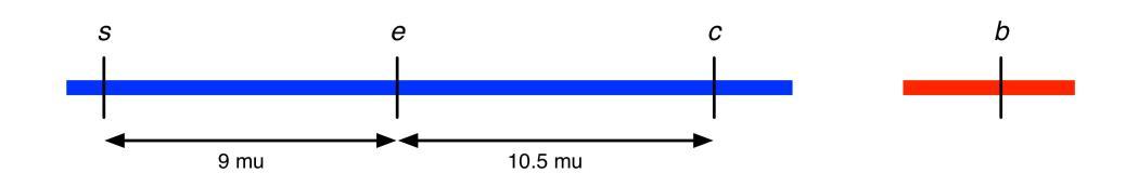
21. The shortest distances are the most accurate. Therefore begin assembling a map using the genes that are closest together. MAT-LEU2 are 16 cM apart and MAT-THR4 are 20 cM apart. This gives two possible maps: MAT - (16 cM) - LEU2/THR4 or LEU2(16 cM) - MAT - (20 cM) - THR4. Because THR4 is 35 cM from LEU2 the second map must be the correct one. Note that the two smaller distances do not sum to the longer distance because these recombination frequencies are based on two-point crosses. The HIS4 gene is 23 cM from LEU2. This initially leads to two possible maps: HIS4 - (23 cM) - LEU2 - MAT - THR4 or LEU2 - (23 cM) - HIS4/MAT - THR4. The first map is the most likely because HIS4 is 37 cM from MAT instead of being very close to MAT. So the order of the genes is HIS4 - LEU2 - MAT - THR4 (or the inverse).

22. In foxgloves, wild-type flower color is red and the mutant color is white; the mutation peloria causes the flowers at the apex of the stem to be very large; normal foxgloves are very tall, and dwarf affects the plant height. When you describe the phenotype of an individual you usually only refer to the non-wild type traits. The cross is: white flowered × dwarf peloria → F1 white flowered × dwarf peloria → 172 dwarf peloria, 162 white, 56 dwarf peloria white, 48 wild type, 51 dwarf white, 43 peloria, 6 dwarf, 5 peloria white.

a. Because there is only 1 phenotype of F1 plant, the parents must have been homozygous for all three genes. The phenotype of the F1 heterozygote indicates the dominant alleles: white flowers , tall stems, and normal-sized flowers.

b. Designate the alleles for the 3 genes: W = white, w = red; P = normal-sized flowers, p = peloria; T = tall, t = dwarf. The cross is: WW PP TT (white flowered) × ww dd pp (dwarf peloria)

No reproduction or distribution without the prior written consent of McGraw-Hill Education.

chapter 5 5-

c. Note that all 3 of these genes are genetically linked. There are only 2 classes of parental progeny as defined both phenotypically and numerically. In order to draw a map of these genes, organize the testcross data (see the Table that follows), figure out which of the 3 genes is in the middle and calculate the recombination frequencies in regions 1 and 2. By definition, the parentals are the class with the same phenotype as the original parents of the cross, and the DCO class is the least frequent reciprocal pair of progeny. At this point, arbitrarily one of the remaining 2 reciprocal pairs of progeny is SCO 1 and the last remaining pair is SCO 2.

Classes of gametes Genotype

Parental W P T 162

Compare the DCO class with the parental class. Remember that a DCO comes from a meiosis with a simultaneous crossover in regions 1 and 2. As a result, the allele of the gene in the middle switches with respect to the alleles of the genes on the ends. In this data set, take one of the DCO classes (for example W p T) and compare it to the most similar parental gamete (W P T). Two alleles out of three are in common; the one that differs (p in this case) is the gene in the middle. Thus, the order is W P T (or T P W).

Once you know the order of the 3 genes, you must calculate the 2 shortest distances - from the end to the center (W↔P) and from the center to the other end (P↔T). The total number of progeny in this testcross = 543. RF W↔P = (56 + 48 + 6 + 5)/543 = 115/543 = 21.2 cM; RF P↔T = (51 + 43 + 6 + 5)/543 = 19.3 cM.

The map is:

d. Interference (I) = 1 - coefficient of coincidence (coc) coc = frequency of observed DCO / frequency of expected DCO

The expected percentage of double crossovers is the product of the RF in each interval: (0.193) × (0.212) = 0.0409. The observed DCO frequency = 11/543 = 0.0203; coc = 0.0203/0.0409 = 0.496; I = 1 - 0.496 = 0.504.

23. Although this problem considers three different genes, each cross only considers two at a time. You are thus asked to construct a map of the three genes based on 3 two-point crosses. Note the unusual usage of a comma to separate the genes in the genotypes written for the parents of each cross. This is meant to show that we don't know if any

No reproduction or distribution without the prior written consent of McGraw-Hill Education.

chapter 5 5-

Numbers

(P) w

w P

w p T

DCO w P t 6 W p T 5

p t 172 SCO 1

p t 56

T 48 SCO 2

of the genes are on the same chromosome. If the two genes in each cross are assorting independently then the four phenotypic classes in the testcross progeny must occur in equal frequencies. This is clearly not the case in any of the three crosses. Therefore the mb, e and k genes are all linked. The genotypes of the parents in the first cross may be correctly written as mb+ e+ / mb+ e+ × mb e / mb e.

In the first cross, the mb+ e+ and mb e classes are the parentals. This is based both on the known genotypes of the true breeding parental generation and on the fact that this reciprocal pair is the most frequent. The recombinants are the mb+ e and the mb e+ flies, so the RF = 11 + 15 / 250 = 0.104 = 10.4 mu. In the second cross the recombinant reciprocal pair is k+ e+ and k e, so the recombination frequency is 11 + 7 / 312 = 0.058 = 5.8 mu. The k mb+ and k+ mb classes are the recombinant reciprocal pair for the third cross. In this case the RF = 11 + 15 / 422 = 0.062 = 6.2 mu. The mb and e genes in the first cross are the furthest apart, so the k gene must be in between them. Thus the map of these data is:

Note that the distance calculated between e and mb in cross one (10.4 mu) does NOT equal the sum of the two shorter distances (12.0 mu). The distance calculated from cross one is less accurate because it is based on single crossovers between e and mb and does not include any of the double crossovers that occurred in the e↔k and k ↔mb regions simultaneously. Thus, the best map of these genes is:

24. Diagram the cross: pink petals, black anthers, long stems × pink petals, black anthers, long stems → the progeny listed in the table.

a. Looking at flower color alone, the cross is pink × pink → (78 + 26 + 44 + 15) red : (39 + 13 + 204 + 68) pink : (5 + 2 + 117 + 39) white = 163 red : 324 pink : 163 white. The appearance of two new phenotypes (red and white) suggests that flower color shows incomplete dominance. This idea is confirmed by the 1:2:1 monohybrid ratio seen in the self-cross progeny. The pink flowered plants are Pp, red are PP and white are pp.

b. The expected ratio of red: pink : white would be 1:2:1. Calculating for the 650 plants, this equals 162.5 red, 325 pink, and 162.5 white

c. The monohybrid ratio of the black and tan anthers = (78+26+39+13+5+2) tan : (44 + 15 + 204 + 68 + 117 + 39) black = 163 tan : 487 black = ~ 1 tan : 3 black. Therefore black (B) is dominant to tan (b) The monohybrid ratio for the stem

No reproduction or distribution without the prior written consent of McGraw-Hill Education.

chapter 5 5-

length = 487 long stems : 163 short stems. = ~ 3 long : 1 short, so long (L) is dominant to short (l).

d. Designate the alleles: PP = red, Pp = pink, p = white; B = black, b = tan, L = long, l = short. Because all 3 monohybrid phenotypic ratios are characteristic of heterozygous crosses, the genotype of the original plant is Pp Bb L l.

e. If the stem length and anther color genes assort independently, the 9:3:3:1 phenotypic ratio should be seen in the progeny. Totaling all the progeny in each of the classes: 365 long black : 122 short black : 122 long tan : 41 short tan. The observed dihybrid ratio is close to a 9:3:3:1 ratio, so the genes for anther color (B) and stem length (L) are unlinked

The expected monohybrid ratio for flower color is 1 red : 2 pink :1 white, while that for stem length is 3 long :1 short. If the two genes are unlinked, the expected dihybrid ratio can be calculated using the product rule to give 3/8 long pink : 3/16 long red : 3/16 long white : 1/8 short pink : 1/16 short red : 1/16 short white, or a 6 L– Pp : 3 L– PP : 3 L– pp : 2 ll Pp : 1 ll PP : 1 ll pp ratio. The observed numbers are: 243 long pink : 122 long red : 122 long white : 81 short pink : 41 short red : 41 short white. This observed ratio is close to the predicted ratio, so the genes for petal color (P) and stem length (L) are unlinked.

The same analysis is done for flower color and anther color. The expected dihybrid ratio here is also 6:3:3:2:1:1. The observed numbers are: 272 black pink : 59 black red : 156 black white : 52 tan pink : 104 tan red : 7 tan white. Because these numbers do not fit a 6:3:3:2:1:1 ratio, we can conclude that flower color (P) and anther color (B) are linked genes.

f. It is clear that the original snapdragon was heterozygous for Pp and Bb. However the genotype of this heterozygous plant could have been either P B / p b or P b / p B If it is the former and the genes are closely linked, then the pp bb phenotype will be very frequent (almost 1/4 of the progeny because it is nonrecombinant). Instead the pp bb class is very infrequent, accounting for only about 1% (7/650) of the progeny. Thus, the parental genotype must have been P b / p B. In this case, the infrequent pp bb class received a p b recombinant gamete from each parent. The frequency of the pp bb genotype = (frequency of the p b recombinant gamete)2. The recombination frequency (RF) between the P gene and the B gene = frequency of P B + p b gametes = 2(√(#pp bb/# total progeny) = 2(√(7/650)) = ~20 map units.

25. a. See Problem 5-29 for a detailed explanation of the methodology. Diagram the cross:

a+ b+ c+ / a b c ♀ × a b c / a b c ♂ → ?.

Recombination occurs in Drosophila females, so the female parent will make the following classes of gametes. Because this is a testcross, these gametes will determine the phenotypes of the progeny. The Table that follows indicates the kinds of gametes that the female parent will produce and their frequencies.

chapter 5

No reproduction or distribution

Education

without the prior written consent of McGraw-Hill

5-25

b. Diagram the cross: a+ b+ c+ / a b c ♂ × a b c / a b c ♀ → ?. Here, the heterozygous parent is the male. Recombination does not occur in male Drosophila. Thus, the heterozygous parent will generate only 2 types of gametes, the parental types. If you score 1,000 progeny of this cross, you will find 500 a+ b+ c+ and

26. First re-write the data as genotypes grouping the genetic reciprocal pairs.

The th h st and wild-type (+ + +) classes are defined as parental because they are the most frequent reciprocal pair.

a. Each class of the parental reciprocal pair corresponds to one homolog of the heterozygous Drosophila female that was testcrossed to the homozygous recessive male. Thus the genotype of this female is th h st / th+ h+ st+ .

b. This is a testcross with three linked genes, but there are only 6 classes of data (3 reciprocal pairs) instead of 8 classes. The missing reciprocal pair is th + + and + h st This pair must be the least frequent DCO class. Comparing the th + + DCO class to the + + + parental class (the most similar) shows that th is the gene that differs, so th must be the gene in the middle. The h ↔th distance is 35 + 34 / 1000 = 0.069 = 6.9 mu. The th ↔st distance is 37 + 33 / 1000 = 0.07 = 7 mu. The best map is:

chapter 5 Copyright

All rights

No reproduction or distribution without the prior written consent of McGraw-Hill Education Classes of gametes Genotype Frequency of reciprocal pair Numbers Frequenc y of each class # of progeny freq x 1,000 Parental (P) a+ b+ c+ a b c 1 - all else 1 - (0.18 + 0 08 + 0 02) = 0 72 0 36 0 36 360 360 SCO 1 a+ b c a b+ c+ RF in region 1 = SCO 1 + DCO SCO 1 = 0 2 - 0 02 = 0 18 0 09 0 09 90 90 SCO 2 a+ b+ c a b c+ RF in region 2 = SCO 2 + DCO SCO 2 = 0 1 - 0 02 = 0 08 0 04 0 04 40 40 DCO a+ b c+ a b+ c (RF in region 1) x (RF in region 2) (0.2) x (0.1) = 0.02 0.01 0.01 10 10

reserved

500 a b c progeny

Classes of gametes Genotype Numbers Parental (P) th h st 432 + + + 429 Recombinant th h + 37 + + st 33 Recombinant th + st 35 + h + 34

c. I = 1 – coefficient of coincidence; coefficient of coincidence = observed DCO / expected DCO. Thus coefficient of coincidence = 0 / (0.069)(0.07) = 0 and I = 1 –0 = 1. The interference is complete.

27. a. wild type ♀ × scute echinus crossveinless black ♂ → 16 classes of data

Among the 16 classes there are wild type for all traits and scute, echinus, crossveinless, and black. This tells you that the parental female was heterozygous for all 4 traits. The fact the parental female is wild type also tells you that the wild- type alleles of all 4 genes are dominant. Remember that if you do a testcross with a female that is heterozygous for 3 linked genes, the data shows a very specific pattern. Because each type of meiosis (no recombination, DCO, etc.) gives a pair of gametes, you will see 8 classes of data that will occur in 4 pairs, both genetically and numerically. Thus, if you begin a cross with a female that is heterozygous for 4 linked genes, you should see 16 classes of progeny in a pattern of 8 genetic and numeric pairs. Although we have 16 classes of data, they do not occur in numeric pairs - instead we see numeric groups of 4. If one (or more) of the genes instead assorts independently of the others, then in a testcross you must see numeric groups of 4. For example, the most frequent classes will be parental, and there will be a 1:1:1:1 ratio of the 4 parental types.

Which gene is assorting independently relative to the other 3 genes? To answer this question, list the genotypes of the gametes that came from the heterozygous parent in the largest group of 4. This group should include the parental classes for the 3 linked genes; there are 4 genotypes here to account for the independent assortment of the unlinked gene. Then choose one of the 4 genes, and remove the allele of that gene from all 4 groups. When you do this with the gene that is assorting independently of the rest, you will find there are only 2 reciprocal classes of data left, which are the parental classes for the linked genes. If you choose one of the linked genes to remove, you will still have 4 different phenotypic classes left.

Try removing the b gene first, as shown in the third column of the Table that follows. You see that when the b allele is removed, only 2 classes are left: s e c and + + +. But when this analysis is repeated removing the allele of the s gene there are still 4 different phenotypes left (see the right column of the Table).

The b gene is therefore assorting independently of the other 3 genes. When the b gene is removed from all 16 classes of data, you can see that the data reduces to 8 classes that form 4 genetic and numeric reciprocal pairs, just as in any three-point cross [see answer to part (b) below]. Thus, the genotype of the parental female is:

No reproduction or distribution without the prior written consent of McGraw-Hill Education.

chapter 5 5-

Genotype Numbers remove b remove s b s e c 653 s e c b e c + s e c 670 s e c + e c + + + + 675 + + + + + + B + + + 655 + + + b + +

b. Write the classes out as reciprocal pairs.

Classes of gametes

Genotype Numbers

Parental (P) + + + 1323 s e c 1330

SCO 1 s + + 144 + e c 147

SCO 2 s e + 171 + + c 169

DCO s + c 2 + e + 2

Compare the DCO s + c to the parental s e c ; this shows that e is in the middle.

Calculate RF s ↔ e = (144 + 147 + 2 + 2)/3288 = 9.0 cM; RF e ↔ c = (171 + 169 + 2 + 2)/3288 = 10.5 cM.

c. Interference = 1 - coefficient of coincidence coc = observed DCO frequency / expected DCO frequency = (4/3288) / (0.09 × 0.105) = 0.001 / 0.009 = 0.11.

I = 1 0.11 = 0.89; yes, there is interference.

28. a. Recombination does not occur in male Drosophila. Therefore, in the cross A b / a B

♀ × A b / a B ♂ → F1, the females will make 4 types of gametes (parental A b and a B; recombinant A B and a b). The frequencies of the 2 parental gametes will be equal to each other, and the frequency of the A B recombinant will be equal to the frequency of its reciprocal recombinant, a b. Males, however, will make only two (parental) gamete types in equal numbers: A b and a B. The Punnett square that follows shows how this will play out; the relative sizes of the boxes do not affect the ultimate answer.

No reproduction or distribution without the prior written consent of McGraw-Hill Education.

chapter 5 5-

There is a ratio of 1/4 A– bb (orange boxes): 1/2 A– B– (blue boxes): 1/4 aa B–(purple boxes) for the progeny receiving the parental gametes AND the same ratio among the progeny receiving the recombinant gametes. Thus, the overall phenotypic dihybrid ratio will always be 1/4 A– bb : 1/2 A– B– : 1/4 aa B–, independent of the recombination frequency between the A and B genes.

This will not be true of the cross A B / a b ♀ × A B / a b ♂ (see Table on the following page). The male will make the parental gametes, A B and a b, while the female will make 4 types of gametes: parental A B and a b; recombinant A b and a B. In this case, half of the progeny will look A– B– because they received the A B gamete from the male parent irrespective of the gamete from the female parent. When the male parent donates the a b gamete, then it is the gamete from the female parent that determines the phenotype of the offspring. The progeny that are A– bb and aa B– have received a recombinant gamete from the female parent (and the a b gamete from the male). These classes of progeny can then be used to estimate the recombination frequency between the A and B genes: RF = 2(# of A– bb + # of aa B–)/total progeny. (The factor of 2 is included because you cannot see half of the recombinants.)

chapter 5 5-29

b. In mice, recombination occurs in both females and males. Therefore, in the cross A b / a B ♀ × A b / a B ♂ both sexes will make the same array of gametes (parental A b and a B; recombinant A B and a b). In this case, the only phenotype of progeny with a singular genotype will be aa bb. In the cross under consideration here, the aa bb phenotype can only arise if both parents donate the a b recombinant gamete. Of course, the other recombinant gamete, A B, occurs with equal frequency. The probability of the aa bb genotype = (probability of an a b recombinant gamete)2. If you know the frequency of the aa bb phenotypic class in the progeny, recombination frequency (frequency of recombinant products) between the A and B genes = 2(√#aa bb/# total progeny).

In the case of the A B / a b ♀ × A B / a b ♂ cross in mice, both sexes are making the same parental gametes (A B and a b) and recombinant gametes (A b and a B) gametes. Again, the only phenotype of progeny with a singular genotype will be aa bb. In this example, this phenotype is the result of the fusion of the a b parental gamete from each parent. The frequency of the aa bb phenotype = (the frequency of the a b gamete) × (the frequency of the a b gamete). If you know the frequency of the aa bb phenotypic class in the progeny, the frequency of nonrecombinant products between the A and B genes = 2(√#aa bb/# total progeny). Recombination frequency = 1 - frequency of nonrecombinant products between the A and B genes.

chapter 5 5-30

reproduction or distribution without the prior written consent of McGraw-Hill Education.

Assume no interference, and remember the map of these 3 genes:

You are being asked to calculate the proportion of the testcross progeny that will have the Virginia parental phenotype. In Chapter 3 we could answer this question by calculating the monohybrid ratios for each pair of alleles (M : m, C : c and S : s) in the heterozygous parent. The testcross parent can provide only the recessive alleles for each gene, so the probabilities of the various phenotypes can be determined by applying the product rule. Unfortunately, this method of arriving at the probability of the progeny phenotypes only works when the genes under discussion are assorting independently. When the 3 genes are linked, as in this problem, to calculate the frequency of a parental class we must calculate first calculate the frequencies of all of the phenotypes expected in the testcross progeny.

A parent that is heterozygous for 3 genes will give 8 classes of gametes. In a test cross, the gamete from the heterozygous parent determines the phenotype of the progeny. When the 3 genes are genetically linked, these 8 classes will be found as 4 reciprocal pairs. In other words, each meiosis in the heterozygous parent must give 2 reciprocal products that occur at equal frequency. For instance, a meiosis with no recombination will produce the parental gametes, M C S and m c s at equal frequency. This particular reciprocal pair will also be the most likely event and so the most frequent pair of products. The least probable meiotic event is a double crossover which is a recombination event in the region between M and C (region 1) and simultaneously in the region between C and S (region 2). The remaining gametes are produced by a single crossover in region 1 (the reciprocal pair known as single crossovers in region 1 or SCO 1) and a single crossover in region 2 (the reciprocal pair known as single crossovers in region 2 or SCO 2).

The numbers shown on the map of this region of the chromosome represent the recombination frequencies in the gene-gene intervals. There are 6 mu between the M and C genes, so 6% (RF = 0.06) of the progeny of this cross will have had a recombination event in region 1. This recombination frequency includes all detectable recombination events between these 2 genes - both SCO in region 1 and DCO. Likewise, 17% of all the progeny will be the result of a recombination event in region 2. The DCO class is the result of a simultaneous crossover in region 1 and region 2. Recombination in two separate regions of the chromosome should be independent of each other, so we can apply the product rule to calculate the expected frequency of DCOs. Thus, the frequency of DCO = (0.06) × (0.17) = 0.01. Remember that the recombination frequency between M and C (region 1) includes both SCO 1 and DCO. Thus, 0.06 = SCO 1 + 0.01; solve for SCO 1 = 0.06 - 0.01 = 0.05. The same calculation

chapter 5 5-31

M C S / M C

× m c s / m c s (Carolina strain) → F1 M C S / m c s × m c s / m c s → ?

reproduction or distribution without the prior written consent of McGraw-Hill Education. 29. Diagram the cross:

S (Virginia strain)

for region 2 shows that SCO 2 = 0.16. The parental class = 1 - (SCO 1 + SCO 2 + DCO). Also remember that each class of gametes (parental, etc.) is made up of a reciprocal pair. If the frequency of the DCO class is 0.01, then the frequency of the M c S gamete is half of that = 0.005. This logic is summarized in the table below.

a. The proportion of backcross progeny resembling Virginia (parental, M C S) = 0.39.

b. Progeny resembling m c s (P) = 0.39.

c. Progeny with M c S (DCO) = 0.005

d. Progeny with M C s (SCO 2) = 0.8

30. On the basis of a recombination frequency (RF) of 5%, the physical distance between the HD gene and the G8 marker was estimated to be 5 million bp, but when the human genome was sequenced, the actual physical distance between the gene and the marker was found to be only 500,000 bp. Why is the actual distance much lower than the estimated distance? The reason is that the estimate of the distance on the basis of the RF assumes that recombination is uniform over the entire genome. This assumption is not true. Although over the whole genome the average relationship is that 1% RF corresponds to 1 million bp everywhere in the genome, this value hides a great deal of variation in the relationship in different regions of the genome.

In this particular case, it appears that about 10× more crossovers occur in the interval between the HD gene and the G8 marker than in the average 500,000 bp interval in the genome. Clearly then, the genomic DNA between HD and G8 contains a recombination hotspot.

31. In cross #1the criss-cross inheritance of the recessive alleles for dwarp and rumpled from mother to son tells you that all these genes are X-linked. In cross #2, you see the same pattern of inheritance for pallid and raven, so these genes are X-linked as well. The fact that the F1 females in both crosses were wild type tells you that the wild-type allele of all four genes is dominant to the mutant allele. Designate alleles: dwp+ and dwp for the dwarp gene, rmp+ and rmp for the rumpled gene, pld+ and pld for the pallid gene, and rv+

5-32

chapter 5

Classes of gametes Genotype Frequency of reciprocal pair Numbers Frequency of each class Parental M C S 1 - all else 1 - (0 05 + 0 16 + 0 39 (P) m c s 0 01) = 0 78 0 39 SCO 1 M c s RF in region 1 = SCO 1 + DCO SCO 1 = 0 06 - 0 01 = 0 025 m C S 0 05 0 025 SCO 2 M C s RF in region 2 = SCO 2 + DCO SCO 2 = 0 17 - 0 01 = 0 08 m c S 0.16 0.08 DCO M c S (RF in region 1) x (RF in region 2) (0.06) x (0.17) = 0.01 0 005 m C s 0 005

and rv for the raven gene. Assign the genes an arbitrary order to write the genotypes. If you keep the order the same throughout the problem, it is sufficient to represent the wildtype allele of a gene with +.

Cross 1: dwp rmp + + / dwp rmp + + × + + pld rv / Y → dwp rmp + + / + + pld rv

(wild-type females) and dwp rmp + + / Y (dwarp rumpled males).

Cross 2: + + pld rv /+ + pld rv × dwp rmp + + / Y → + + pld rv / dwp rmp + +

(wild-type females) and + + pld rv / Y (pallid raven males).

Final cross: dwp rmp + + / + + pld rv (cross 1 F1 females) × dwp rmp pld rv / Y → 428

+ + pld rv, 427 dwp rmp + +, 48 + rmp pld rv, 47 dwp + + +, 23 + rmp pld +, 22 dwp + + rv, 3 + + pld +, 2 dwp rmp + rv.

All 4 genes might be genetically linked, as they are all on the X chromosome. If so, you expect 16 classes of progeny (2 × 2 × 2 × 2) in 8 genetic and numeric pairs. Notice that there are only 8 classes of progeny. The data that is seen shows exactly the pattern you expect for a female that is heterozygous for 3 linked genes. If 2 of the 4 genes never recombine then you would expect the pattern of data that is seen. If 2 genes never recombine, they will always show the parental configuration of alleles. Thus, examine the various pairs of genes for the presence or absence of recombinants. Note that you never see recombinants between pallid and dwarp: all the progeny are either pallid or dwarp, but never pallid and dwarp nor wild type for both traits. This suggests that the two genes are so close together that there is essentially no recombination between the loci. If a much larger number of progeny were examined, you might observe recombinants. Treat dwp and pld as 2 genes at the same location, so one of them (dwp, for instance) can be ignored, and this problem becomes a three-point cross between pld, rv and rmp.

When the rmp + rv DCO class is compared to the rmp + + parental class, you can see that rv is in the middle. The rmp ↔ rv RF = (48 + 47 + 3 + 2)/1000 = 10 cM; the pld ↔ rv RF = (22 + 23 + 3 + 2)/1000 = 5 cM I = 1 - coc; coc = observed frequency of DCO/expected frequency of DCO. Thus, coc = (5/1000)/(0.05)(0.1) = 0.005/0.005 = 1; I = 1 - 1 = 0, so there is no interference.

5-33

No reproduction or distribution without the prior written consent of McGraw-Hill Education.

chapter 5

Classes of gametes Genotype Numbers Parental (P) dwp rmp + + 427 + + pld rv 428 SCO 1 + rmp pld rv 48 dwp + + + 47 SCO 2 dwp + + rv 22 + rmp pld + 23 DCO + + pld + 3 dwp rmp + rv 2

32. a. Interference is a phenomenon by which the occurrence of one crossover prevents the occurrence of a second crossover in a nearby region of the same chromosome. Scientists think that the existence of interference helps ensure that each bivalent has at least one crossover, which is necessary in turn to ensure that homologous chromosomes segregate from each other properly during the first meiotic division. One way of thinking about the utility of interference is the following: If you assume that only a limited amount of recombination enzymes are available in primary spermatocytes or primary oocytes, the limited number of crossovers that can occur will be apportioned among all the bivalents.

Fig. 5.7a on p. 134 shows a preparation of chromosomes from a primary spermatocyte. Note that each bivalent shows at least one green recombination nodule (a few may be hard to see, but they are present). The existence of interference is suggested by the fact that even on the bivalents that show more than one spot of recombination nodules, these nodules are far away from each other. That is, one recombination event prevents the occurrence of a nearby recombination event on the same bivalent.

b. Figure 5.7a merely suggests that two crossover events do not occur often at nearby positions on the same bivalent. To show that this conclusion about the existence of interference actually hold up from this type of evidence, you would have to look at many meiotic figures from many spermatocytes and/or oocytes. You would then have to ask: If recombination nodules can occur at any position in the genome with equal likelihood (that is, if interference did not exist), how likely would it be that two recombination nodules would occur in a given specified distance on one bivalent. (You could calculate this probability by totaling the average number of recombination nodules from many meiotic figures and dividing by the total length of all the chromosomes to find the average distance between nodules. You could then see if the space between nodules can be graphed as a normal (Gaussian) distribution around this average. If the data did not resemble the expected bell-shaped curve, then the distribution is not random. If interference did exist, you would expect to see the data shifted over from a bellshaped curve so as to favor larger-than-average distances between adjacent nodules.

33. To answer this question, you need first to count the number of recombination nodules visible in the whole genome depicted in Fig. 5.7a on p. 134. There is at least one nodule per bivalent, and there are 20 bivalents in mice. By our own count, we see 29 nodules, but you may see (or imagine you see) a few more or less. We will take 29 as the proper count here. In this meiotic figure, the 29 nodules are distributed among 1,386 cM in the male genetic map. If the same mouse genome corresponds to 1,817 cM in the female genetic map, this must be because more recombination events take place in the average primary oocyte than in the average primary spermatocyte. So you would multiply 29 times the ratio of the cM in the female : male genetic maps (1,817 / 1,386) = ~38 recombination nodules in the average prophase I primary oocytes. [Your final answer may vary depending on how many nodules you counted in Fig. 5.7a, but your answer must be more than 20 × (1,817 / 1,386) = 26.]

5-34

chapter 5

Section 5.4

34. The null hypothesis is that there is independent assortment of 2 genes yielding a dihybrid phenotypic ratio of 9/16 R– Y– : 3/16 R– yy : 3/16 rr Y– : 1/16 rr yy Use the chi square (Χ2) test to compare Mendel's observed data with the 9:3:3:1 ratio expected for two genes that assort independently.

The number of classes is 4, so the degrees of freedom is 4 1 or 3. Using Table 5.2 on p. 147 of the text, the probability of having obtained this level of deviation by chance alone is between 0.9 and 0.99 (90 - 99%). Thus we cannot reject the null hypothesis. In other words, the data are consistent with independent assortment and we therefore conclude that Mendel's data could indeed result from the independent assortment of the 2 genes.

You should note, however, that although Mendel’s data are consistent with independent assortment, this chi square analysis does not prove that these genes assort independently. This analysis did not exclude any hypothesis. We could not formulate the null hypothesis as stating that the genes do not assort independently; we cannot predict the expected number of progeny under this hypothesis given that linked genes can have RF anywhere from 0% to just under 50%.

35. a. Diagram the cross.

B–) → F1 brown (O– B–) → 100 brown (O– B–) : 25 orange (O– bb) : 22 black (oo B–) : 13 albino (oo bb)

Because the F1 snakes were all brown, we know that the orange snake could not have contributed an o allele, or there would have been some black snakes. The orange snake must be OO bb The black snake could not have contributed a b allele or there would have been some orange snakes, so the black parent must be oo BB. Therefore the F1 snakes must be Oo Bb.

b. The F1 snakes are heterozygous for both genes (Oo Bb). If the two loci assort independently, we expect the F2 snakes to show a 9 brown : 3 orange : 3 black : 1 albino ratio. The total number of F2 progeny is 160. We expect 90 (160 × 9/16) of these progeny to be brown, 30 (160 × 3/16) to be orange, 30 to be black and 10 (160 × 1/16) to be albino

5-35

No reproduction or distribution without the prior written consent of McGraw-Hill Education.

chapter 5

Genotypes Observed # Expected # Χ2 equation Sum of Χ2 R– Y– 315 9/16 (556) = 313 (315 313)2/313 0.01 R– yy 108 3/16 (556) = 104 (108 104)2/104 0 15 rr Y– 101 3/16 (556) = 104 (101 104)2/104 0 09 rr yy 32 1/16 (556) = 35 (32 35)2/35 0.26 0.51

orange (O– bb) × black (oo

There are three degrees of freedom (4 classes 1) and the p value is between 0.5 and 0.1. The observed values do not differ significantly from the expected.

d. There is a 10% - 50% probability that these results would have been obtained by chance if the null hypothesis were true; this is simply another way of writing the meaning of the p value.

36. a. The cross is: normal (DD) × dancer (dd) → F1 normal (Dd) F2 3/4 D– (normal) : 1/4 dd (dancer)

1/4 of the F2 mice will be dancers if the trait is determined by a single gene with complete dominance.

b. Diagram the cross: normal (AA BB) × dancer (aa bb) → F1 normal (Aa Bb) F2 15/16 normal (A–B– + A– bb + aa B–) : 1/16 dancer (aa bb)

1/16 of the mice would be expected to be dancers given the second hypothesis that dancing mice must be homozygous for the recessive alleles of two genes.

c. Calculate the chi square values for each situation. Null hypothesis #1: Dancing is caused by the homozygous recessive allele of one gene, so 1/4 of the F2 mice should be dancers. Calculating the expected numbers, 1/4 × 50 mice or 13 should have been dancers, 37 should have been nondancers.

With one degree of freedom the p value is between 0.5 and 0.1 and we cannot reject the null hypothesis. The hypothesis that dancing is caused by the homozygous recessive allele of one gene is therefore a good fit with the data. Null hypothesis #2: Dancing is caused by being homozygous for the recessive alleles of two genes (aa bb), so 1/16 of the F2 mice should be dancers.

No reproduction or distribution without the prior written consent of McGraw-Hill Education.

5-36

chapter 5 c. Genotypes Observed # Expected # Χ2 equation Sum of Χ2 O– B– 100 90 (100 90)2/90 1.11 O– bb 25 30 (25 30)2/30 0 83 Oo B– 22 30 (22 30)2/30 2.13 oo bb 13 10 (13 10)2/10 0 9 4.97

Genotypes Observed # Expected # Χ2 equation Sum of Χ2 nondancers 42 (3/4) x 50 = 37 (42 37)2/37 0.68 dancers 8 (1/4) x 50 = 13 (8 13)2/13 1 92 2 60

With one degree of freedom, the p value is < 0.005, so the null hypothesis that two genes control the dancer phenotype is not a good fit; in fact, the hypothesis can be rejected by the criteria employed by most geneticists. The one gene hypothesis is a better fit with the data.

Section 5.5

37. a. The number of meioses represented here is the total of the number of asci = 334. Each ascus contains the 4 products of one meiosis.

b. Diagram the cross: a + c × + b +

To map these genes, use the Three Easy Rules for Tetrad Analysis First designate the type of asci represented. This has to be done for each pair of loci as PD (P), NPD (N) and T refer exclusively to the relationship between two genes. In the table below, the top row shows the designations for all three pairs: the a-b comparison is at the lower left, the b-c comparison is at the lower right and the a-c comparison is at the top of the pyramid.

Rule #1: For genes a and b PD = NPD, so these two genes are not linked. For genes b and c PD = NPD, so genes b and c are not linked. For genes a and c, PD>>NPD, so the genes are linked. Calculate RF between a and c = 2 + (1/2)(26 + 25)/334 = 8.2 cM (Rule #2)

Gene-centromere distances can be calculated in Neurospora (Rule #3), so analyze the data for MI and MII segregation patterns for the alleles of each gene in each ascus type. This analysis is done separately for each gene, unlike the gene↔gene analysis done above. The designation for each gene is presented under that gene at the bottom row of the table (I - MI, II = MII). Rule #3 shows that the distance between a and the centromere = (1/2)(26 + 25)/334 = 7.6 mu; the distance between b and the centromere = (1/2)(3)/334 = 0.4 mu; the distance between c and the centromere = (1/2)(0)/334 = 0.

Now compile all of these pieces of data into one map. Rule #1 shows that gene b is 0.4 mu from the centromere and is on a different chromosome from genes a

5-37

All

or distribution

Education. chapter 5 Genotypes Observed # Expected # Χ2 equation Sum of Χ2 nondancers 42 47 (42 47)2/47 0.53 dancers 8 3 (8 3)2/3 8 33 8.86

rights reserved

reproduction

without the prior written consent of McGraw-Hill

P P T T N P P P N N T P T N N P T T a + c a b c + + c + b c a b + a + c a + c a b c a + c a b c a b + a b c + b + + + + + b + + + + + + c + + + + b + + + + a b + a + + + + c + b + 137 141 26 25 2 3 I I I I I I II I I II I I I I I I II I

and c. Genes a and c are on the same chromosome, so the a↔centromere distance and the c↔centromere distance refer to the same centromere. Gene c is 0 mu from the centromere. As you can see from the map, there are 2 slightly different distances for the gene a↔gene c region. The gene↔gene distance is 8.2 mu and the a↔centromere distance is 7.6 mu. In this case the longer gene↔gene distance is more accurate as it includes the SCOs between a and c as well as some of the DCOs between a and c (the 4-strand DCO, Fig. 5.23 on p. 153).

c. Carefully consider the information you have for the different chromosomes in the ascus type chosen (the group with 3 members). The a and c genes show PD segregation, which can mean either no crossing-over between them or a 2-strand DCO. Both genes show MI segregation, which means there haven't been any single crossovers between either gene and the centromere. Gene b shows MII segregation, which means there has been an SCO between the gene and the centromere. This crossover also means the a-b and c-b comparisons in this class will show the tetratype pattern (T are due to crossovers between either gene and its centromere when the genes are on separate chromosomes).

5-38

chapter 5

Classes of gametes Genotype Numbers Parental α + + 31 (P) a f g 29 SCO 1 a + g 6 α f + 6 SCO 2 α + g 13 a f + 14 DCO a + + 1 α f g 1

38. a. These data are presented as phenotypes of individual spores. Because the data are presented for 3 genes, they may be analyzed as a 3-point cross. Organize the data into reciprocal pairs of spores.

The α f g DCO spore type is most similar to the a f g parental spore type. Thus, the mating type (a/α) is the gene in the middle. The distances are: f ↔a/α = (6 + 6 + 1 + 1)/101 = 13.9 cM and a/α↔ g = (13 + 14 + 1 + 1)/101 = 28.7 cM.

b. This problem says you have an ascus with an α f g spore. This spore is the result of a double crossover [see part (a)]. The reciprocal product would be the a + + spore, but this is not seen in the ascus. Remember that there are 3 different types of double crossovers: 2-strand DCOs, 3-strand DCOs, and 4-strand DCOs. Each of these types of DCOs gives a different array of spores in the resulting ascus (Fig. 5.23 on p. 153). Draw a meiotic figure of this chromosome and try some different types of DCOs. A 3-strand DCO gives the desired result.

39. Diagram the cross and summarize the data: met- lys- × met+ lys+ P T

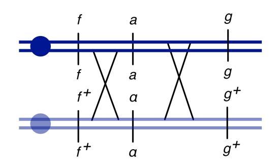
lys+ met+ lys+

lys+ met- lys+ met- lys- met+ lysmet- lys- met- lys89 11

a. The two types of cells in the first group of 89 asci are met+ lys+ (could grow on all four types of media) and met- lys- (require the addition of met and lys to minimal medium). These asci are parental ditypes (PD). The four types of cells in the second group of 11 asci are met+ lys+; met+ lys- (grew on min + lys and on min + lys + met); met- lys+(grew on min + met and on min + lys + met); and met - lys-. These are tetratype (T) asci.

b. Because the number of PD>>> NPD, the genes are linked. The distance between them is: [NPD + (1/2)T] / total tetrads = [0 + (1/2)(11)]/100 × 100 = 5.5 m.u.

c. NPD should be seen eventually and would result from four-strand double crossovers. There would be two types of spores: met - lys+ (could grow on min +

No reproduction or distribution without the prior written consent of McGraw-Hill Education.

chapter 5

5-39

met+

met and on min + met + lys) and met+ lys- (could grow on min + lys and on min + met + lys).

40. Use the Three Easy Rules for Tetrad Analysis to help you solve this problem.

a. In cross 1, the number of PD (parental ditypes) = NPD (nonparental ditypes) so the ad gene and the mating type locus assort independently. In cross 2 the number of PD >> NPD so we can conclude the p gene and the mating locus are linked; RF p↔mating type = [NPD + (1/2)T]/ total tetrads = (3) + (1/2)(27)/54 =16.5/54= .31 × 100 = 31 cM between the two genes.

b. To calculate gene↔centromere distances you need information on the order of ascospores in each ascus type. Only with this information can you calculate gene↔centromere distances based on 1/2(# of asci showing MII segregation for the gene)/total asci.

41. a. The genotype of a true-breeding wild-type diploid strain of Saccharomyces can be written + / +. If this diploid undergoes meiosis, all (100%) of the asci will have 4 viable spores.

b. The genotype of this strain is + / n, where n = a null activity allele of an essential gene. The diploid cells will be viable, because they have functional enzyme for this essential gene from the + allele. If this diploid undergoes meiosis, then all (100%) of the tetrads will have 2 + : 2 n spores (that is, only 2 spores in each tetrad will be viable).

c. Gene a and gene b are different essential genes; a and b represent temperaturesensitive alleles of these genes. When you diagram a cross you must write complete genotypes for both haploid parents: a b+ (strain a) × a+ b (strain b) → aa+ bb+ Each haploid parent strain will die when grown under restrictive conditions because they cannot produce a required product, while the diploid cells are viable because they have a wild-type allele for both genes.

If these genes are unlinked, then after meiosis PD asci = NPD asci (Three Easy Rules for Tetrad Analysis: Rule #1). When the genes are unlinked, also remember that T tetrads (asci) arise from SCOs between either gene and the centromere. Because each of these genes is 0 mu from the centromere, you will not see T asci. Thus, after meiosis, you will have 50% PD (2 a b+ spores : 2 a+ b spores) : 50% NPD (2 a+ b+ : 2 a b). None of the spores in the PD tetrads are viable under restrictive conditions, while 2 of the 4 spores in the NPD asci are viable (a+ b+). Thus, 50% of the asci will have 0 viable spores (PD) and 50% of the asci will have 2 viable spores (NPD).

d. Again genes a and b are unlinked essential genes, but now gene a↔centromere = 0 mu and gene b↔centromere = 10 mu. A SCO between gene b and the centromere

No reproduction or distribution without the prior written consent of McGraw-Hill Education.

chapter 5 5-

will happen in 20% of the asci (because only half of the ascospores of an SCO are recombinant) and will give T asci. A T ascus will have a spore ratio of 1 a+ b+ : 1 a b : 1 a b+ : 1 a+ b. There is 1 viable spore (a+ b+) in a T ascus. The remaining 80% of the asci will be divided equally between PD and NPD because the genes are unlinked. Thus, 40% of the asci will have 0 viable spores (PD), 40% of the asci will have 2 viable spores (NPD) and 20% of the asci will have 1 viable spore (T)

e. Because both genes are on the same chromosome, you can diagram this cross: a b+ (strain a) × a+ b (strain b) → a b+ / a+ b. When the genes are linked, SCO and 3strand DCO between the genes give T asci and 4-strand DCO between the genes gives NPD asci. The remainder of the asci are PD (no crossover and 2-strand DCO). If the recombination frequency between gene a and gene b = 0 mu, then the only possible result will be PD asci (2 a b+ : 2 a+ b) in which none of the spores are viable. Thus, 100% of the asci will have 0 viable spores

f. Now the genes are 10 mu apart and there are no DCO events. This means that 20% of the asci produced will be T [see part (d)] and the remaining 80% will be PD. Therefore, 80% of the asci will have 0 viable spores (PD) and 20% of the asci will have 1 viable spore (T).

g. A 4-strand DCO gives an NPD ascus. The genotypes of the spores will be 2 a+ b+ : 2 a b. Thus, 2 of the 4 spores will be viable.

42. Genes a, b, and c are all on different chromosomes. [For simplicity, we will refer to the centromere of the chromosome on which a gene is found with the possessive (that is, as the gene’s centromere.)] Thus, all crosses between these genes are expected to give an equal number of PD and NPD asci. The fact that the cross involving genes a and b yields no T indicates that genes a and b are both very close to their respective centromeres. If two genes are on separate chromosomes, tetratypes arise when a crossover occurs between one of the genes and its centromere, or between the other gene and its centromere. In the crosses involving genes a and c or genes b and c, many T asci are seen. Because genes a and b are tightly centromere-linked, gene c must be very far from its centromere in order to generate these T asci.

43. Diagram the yeast cross:

his- lys+ × his+ lys- → his- lys+/ his+ lys- → 233 PD, 11 NPD, 156 T.

a. The PD asci must have 2 his- lys+ : 2 his+ lys- spores, the NPD asci have 2 his+ lys+ : 2 his- lys- spores and the T asci have 1 his- lys+ : 1 his+ lys- : 1 his+ lys+ : 1 his- lys- spores

b. PD>>NPD so the genes are linked; RF between 2 genes = [11 + (1/2)(156)]/400 = 22.3 mu

c. Because the genes are linked, you know that NPD asci are the result of 4-strand DCOs. This sort of DCO is 1/4 of all the DCO events. The 3-strand DCOs (1/2 of all DCOs) give T while 2-strand DCOs (1/4 of all DCOs) give PD. In the data you see 11 NPD tetrads, or 11 meioses that underwent 4-strand DCOs. There are another 22 tetrads that are the result of 3-strand DCOs (and are Ts), and another 11

chapter 5 5-

asci that underwent 2-strand DCOs (and are PDs), for a total of (11 + 22 + 11 =) 44 asci that underwent 2 crossovers. The remaining (156 - 22 =) 134 T asci underwent a SCO, or 1 crossover, and the remaining (233 – 11 =) 222 PD asci underwent 0 crossovers (NCOs). From this analysis, you can see that a general equation for the number of SCO meioses is SCO = T-2NPD. Likewise, a general equation for the number of DCO meioses is DCO = 4NPD.

d. There are 44 asci that underwent DCOs for a total of 88 crossover events. There were another 134 asci that underwent SCOs. Thus, there were 134 + 88 = 222 crossover events / 400 meioses = 0.555 crossovers/meiosis. We have just calculated “m”, the mean number of crossovers between his and lys per meiosis. A general equation for m is: m = [(SCO + 2 (DCO)]/total asci.

e. The equation for recombination frequency between 2 genes used in the textbook and in part (b) above only includes 4-strand DCO (NPD). This formula ignores 3strand and 2-strand DCOs. This calculation for recombination frequency assumes that all T asci are due to SCOs. Though this is true for the majority of T asci, some T asci are due to 3-strand DCO events; the larger the distance between the 2 genes in question, the more Ts are due to DCOs. Also, it is an oversimplification to assume that all PD asci are nonrecombinant, because some of them are due to 2strand DCOs; the fraction of PDs due to DCOs also increases with the distance between the two genes in question. Remember that the 3 types of DCO events occur in a ratio of 1 (2-strand DCOs) : 2 (3-strand DCOs) : 1 (4-strand DCOs)(see Fig. 5.23 on p. 153).

A more accurate formula for RF between two genes that takes into account all crossovers is: RF = m/2, where m is the mean number of crossovers per meiosis, as defined in part (d) above. The reason is that every meiosis that occurs with a single crossover (every SCO) results in 2 recombinant chromosomes and 2 nonrecombinants. You can prove to yourself that this equation makes sense by imagining two theoretical situations. First, suppose that every meiosis were an SCO (m = 1); then RF = 1/2 or 50%, as expected when no NCOs occur. Second, suppose that half of all meioses occurred as SCOs (m = 1/2) and the other half were NCOs; then RF = 25%, which makes sense as 1/4 of all resulting chromosomes would be recombinants. (Note that the equation for the green line in Fig. 5.15 on p. 142 is m/2.)

With this understanding, and also the relationships we determined in parts (c) and (d), we can derive a more accurate formula for recombination frequency: RF = m/2 = (1/2 SCO + DCO)/total asci = [1/2 (T – 2NPD) + (4NPD)]/total asci = [(1/2)T + 3NPD]/total asci. Many yeast geneticists use this more accurate formula in preference to the one in your textbook.

f. RF = [(1/2)(156 – 22) + 4(11)]/400 = [(1/2)(134) + 44]/400 = 111/400 = 0.278 = 27.8 mu As you can see, this value is somewhat larger than the distance calculated in part (b). As expected, this corrected RF value = m/2, where m = 0.555 [see part (d)].

44. This problem can be solved only if you make assumptions about interference in the 22 m.u. interval between genes C and D. The reason that interference is important is that the degree of interference determines the number of double crossovers (DCOs) that

No reproduction or distribution without the prior written consent of McGraw-Hill Education.

chapter 5 5-

occur, and this will of course influence the proportion of tetrads that are PD, NPD, and T. The solution is by far easiest to calculate if interference = 1, because no DCOs occur in this situation. We will thus discuss each of the two parts of this problem first under the assumption that interference = 1. We then consider each part of the problem at the other extreme, in which interference = 0. If interference is greater than 0 but less than 1, the proportions of the three types of tetrads would vary between these extremes.

a1. Situation: Cross in Saccharomyces cerevisiae; Interference = 1. Because there are no double crossovers (DCOs) between genes C and D; there can be no NPD tetrads. All the recombinants between the 2 genes are due to single crossovers (SCO). If two genes are linked, then SCOs between the genes give T asci. Remember that the RF between C and D is (.07 + .15 = 0.22), and that the formula for recombination frequency between 2 genes = [NPD + (1/2)T]/total asci. Solve for T: 0.22 = 0 + (1/2)T so T = 2(0.22) = 0.44. Therefore, 44% of the asci will be Ts and the remaining 56% will be PDs. In Problem 43 above you just derived a more accurate formula for RF = [3NPD + (1/2)T]/total asci. This new formula accounts for the Ts and NPDs produced by DCOs, and you can see that when there are no DCOs, both formulas are equally accurate.

b1.Situation: Cross in Neurospora crassa; Interference = 1. In Neurospora the recombination events that underlie the formation of PD, NPD, and T are the same as in yeast. The difference is that the ordered tetrads allow you to distinguish whether a SCO event occurs between C and the centromere or between D and the centromere. If the SCO occurs between C and the centromere, then you will see MII segregation for the alleles of the C gene and MI segregation for the alleles of the D gene. If the SCO occurs between D and the centromere then you will see the reverse - MI segregation for C and MII segregation for D.

Here, I = 1, so there are no DCOs. Therefore, as in part (a), T = 0.44 and PD = 0.56. However 7/22 of the SCO events occur between gene C and the centromere, while the remaining 15/22 of the SCOs occur between D and the centromere. The expected results are summarized in the table below.

Crossover type and location:

NCO (no crossover) SCO C↔cent SCO D↔cent

Before looking at the math for situations where the interference is not equal to 1, you should think about this problem qualitatively. As interference decreases, a higher proportion of meioses will have two or more crossovers. Because NPDs can be produced only by meioses with more than one crossover (in the parts of the problem solved above for interference = 1, there were no NPDs), as interference decreases you will see more NPD tetrads. Because in the corrected equation for RF in tetrad analysis from Problem 43 {where RF = [3NPD + (1/2)T]/total asci}, if the RF was constant, the proportion of T tetrads would have to decrease to compensate for the NPDs. This

chapter 5 5-43

PD T T MI or MII gene C: MI MII MI MI or MII gene D: MI MI MII 0 56 7/22 x 0 44 = 0 14 15/22 x 0 44 = 0 30 frequency:

ascus type:

equation also sets limits on the proportions of the total tetrads that would be T and NPD. Understanding the qualitative relationship of interference with the proportions of tetrads is more important than obtaining numerical values for these proportions, as we next describe.

a2.Situation: Cross in Saccharomyces cerevisiae; Interference = 0. You should note at the outset that the figure accompanying this problem is somewhat ambiguous: Do the map units shown correspond to the measured recombination frequency (RF) in an experiment, or are they instead corrected map units corresponding to the physical distance between the genes (as in Fig. 5.15 on p. 142)? To match all the other problems in this chapter, we assume that the map units shown on the figure represent RFs measured in an experiment. (This ambiguity does not exist when the interference = 1 because the two definitions are then identical.)

If there is no interference, then the likelihood that crossovers occur anywhere on the chromosome is given by a Poisson distribution. Although mathematical methods exist to predict the frequencies of single, double, and higher level crossovers in chromosomal intervals of given lengths from the Poisson distribution, we will simplify the discussion by using an approximation for the expected frequencies of DCOs based on the idea that the two single crossovers occurred independently. That is, the expected frequency of DCO = (recombination frequency in the C↔D region) × (recombination frequency in the C↔D region) = (0.22) × (0.22) = 0.0484. [You may ask why you could not estimate the expected frequencies of DCOs by multiplying the C↔centromere and centromere↔D distances (0.07) x (0.15). The reason is that such a calculation would ignore all the DCOs in which two crossovers take place either in the C↔centromere or in the centromere↔D intervals.]

The RF between C↔D = SCO + DCO (looking at individual spores). [The reason this is true is that even though DCOs have two crossovers, on average, only half of the spores from meioses with double crossovers could be recognized as recombinants.] Thus, 0.22 = SCO + 0.0484; SCO = 0.22 - 0.0484 = 0.1716. If SCO frequency between C and D = 0.1716 then T due to SCO = 0.3432 (see the case above where Interference = 1).

Remember that when analyzing tetrads the three different types of DCOs can be distinguished: 2-strand DCOs, which give PD asci; 3 strand DCOs, which give T asci; and 4-strand DCOs, which give NPD asci (Fig. 5.23b-f on p. 153). These DCOs occur in the ratio of 1/4 (2 strand DCOs) : 1/2 (3-strand DCOs) : 1/4 (4strand DCOs). If the total DCO frequency = 0.0484 then 1/4 (0.0484) = 0.0121 is the frequency of 4-strand DCOs (NPD), 1/2 (0.0484) = 0.0242 is the frequency of 3-strand DCOs (T) and the remaining 1/4 of the DCOs (0.0121) are 2-strand DCOs, which will be PD tetrads.

In total, NPD = 0.0121, T = 0.0242 (due to DCO) + 0.3674 (due to SCO) = 0.3795 and the remainder are PD = 0.6205

b2.Situation: Cross in Neurospora crassa; Interference = 0. Here, the proportions of PD, NPD, and T tetrads will be the same as in part (a2) above. However, several patterns of MI and MII segregation patterns for the two genes are possible depending upon where the SCO and DCO events are occurring. Let’s first consider

chapter 5 5-44

the NCO and SCO meiosis (this is the same table as shown in part [b] above but without the frequencies):

crossover type and location:

ascus type: PD T T gene C (MI/MII) MI MII MI gene D (MI/MII) MI MI MII

Next we consider DCO meioses in which both crossovers occur in the same interval: either C↔centromere or centromere↔D. In either case, the DCO could either involve 2, 3, or 4 strands.

Finally, let’s look at the DCO meioses in which one crossover occurs in C↔centromere and the other crossover occurs in centromere↔D. Such DCOs could again involve either 2, 3, or 4 strands.

Note that in these tables, we have calculated the frequencies only for the DCOs in which one crossover occurs in C↔centromere and the other crossover occurs in centromere↔D. In this situation, the expected number of simultaneous crossovers in both regions is easy to calculate as the product of the map distances in the two intervals (0.07) x (0.15) = 0.0105. The number of meioses with 3-strand DCOs will be twice that of the meioses with either 2-strand or 4-strand DCOs. The frequencies for the classes shown in the two previous tables are complex to calculate (for example, you would have to determine the expected number of DCOs with both crossovers in each interval) and are not worth the effort. What is worthwhile is to look at the patterns of PD, NPD, and T superimposed with the

No reproduction or distribution without the prior written consent of McGraw-Hill Education.

chapter 5 5-

crossover SCO C↔

cent SCO cent.↔D

crossover type and location: DCO C↔cent 2-strand DCO C↔cent 3-strand DCO C↔cent 4-strand DCO cent.↔D 2-strand DCO cent.↔D 3-strand DCO cent.↔D 4-strand ascus type: PD T NPD PD T NPD gene C (MI/MII) MI MII MI MI MI MI

MI MI MI MI MII MI

gene D (MI/MII)

crossover type and location: DCO C↔cent cent.↔D 2-strand DCO C↔cent cent.↔D 3-strand DCO C↔cent cent.↔D 4-strand ascus type: PD T NPD gene C (MI/MII) MII MII MII gene D (MI/MII) MII MII MII frequency: 1/4 x 0.0105 = 0 003 1/2 x 0.0105 = 0 005 1/4 x 0.0105 = 0 003