REVIEW OF THE EFFECTS OF STANDARD DEVIATION ON TIME AND FREQUENCY RESPONSE OF GAUSSIAN FILTER

REVIEW OF THE EFFECTS OF STANDARD DEVIATION ON TIME AND FREQUENCY RESPONSE OF GAUSSIAN FILTER

Hyginus Udoka Eze, Martin C. Eze, Chidume S. Chidiebere, Bassey Okon Ibokette,

Ani, Uchenna P. Anike

Abstract - This research reviews the effects of a standard deviation on time response and frequency response of Gaussian filter. In the research, standard deviations of 0.5, 1, 1.5, 2, 2.5 and 3 were applied to normalized Gaussian filter in time domain and frequency domain. From the result of the simulation, it was observed that in the time domain, the peak amplitude of the filter increased with a decrease in the standard deviation and the execution time decreased with a decrease in standard deviation. In the frequency domain, the peak amplitude is constant for all the standard deviation and the frequency bandwidth decreased with increase in standard deviation. The simulation was carried out using Matrix Laboratory (MatLab).

Index Terms - Frequency Domain, Frequency Response, Gaussian Filter, Peak Amplitude, Standard Deviation, Time Response

1.1. Introduction

The Gaussian filters find widespread application in signal processing because Gaussian masks have non-negative values (h (t) ≥ 0) for the range -∞ < t < ∞, and, therefore, do not invert the filtered signal. It is one of the best signals filtering method based on the Gaussian distribution invented by a German mathematician, Carl Friedric Gauβ. Gaussian filter is a non-causal filter which has found applications in low-level computer vision [1] and pattern recognition which includes, image clustering, anomaly detection, classification, regression and principal component analysis [2] The Gaussian filter is a non-zero function that theoretically requires an infinite window length �������� [ ∞ , ∞] for precise filter implementation. The geometric distribution of the mapped time coordinates in kernel space of a Gaussian distribution depends on the standard deviation (σ). The standard deviation of the Gaussian function plays an important role in the filter

IJSER

behaviour. The size of a Gaussian filter determines the standard deviation needed for effective filtering. The σ needed is directly proportional to the filter size. The selection of an appropriate value of standard deviation (σ) for different Gaussian filter sizes, is known as tuning [2]. For optimum tuning, the value of σ must not be too big or too small, but must minimize intra-class variation and maximize inter-class variation [4] and at the same time reduces the execution time. The standard deviations for different Gaussian filter sizes are obtained from (1) where M is the size of the filter. ���� = ����− 1 6 (1)

Equation (1) shows that the standard deviation value for optimum performance increases with the length of the filter. It can be shown that large filter size needs the large standard deviation, for effective filtering. The comprehensive statistical properties of the Gaussian filter create an approach for the Gaussian filter tuning and design.

• Hyginus udoka Eze is a masters’ degree holder in electronic engineering in University of Nigeria, Nsukka. Nigeria E-mail: ezehyginusudoka@gmail.com

• Martin C Eze is currently pursuing Phd program in electronic engineering in University of Nigeri Nsukka, Nigeria, E-mail: martin.eze@unn.edu.ng

• Chidume S Chidiebere is a masters’degree holder in electronic engineering in University of Nigeria, Nsukka. Nigeria. E-mail:chidumechidieberesunday@gmail.com

• Bassey Okon Ibokette is a masters’ degree holder in lectronic engineering in University of Nigeria, nsukka. Nigeria. E-mail;basseyibokette@gmail.com

• Micheal Ani is currently pursuing Phd program in electronic engineering in Univeristy of Nigeria, Nsukka. Nigeria. E-mail:micanian4real@gmail.com

• Uchenna p Anike is a masters’ degree holder in electronic engineering in Univeristy of Nigeria, Nsikka.. Nigera. E-mail: anikeuc@yahoo.com

When the filter size is constant, the variation of standard deviation affects the bandwidth, execution time, and amplitude of the filter. A filter with a narrow bandwidth is used where a very narrow frequency band is needed from a broad spectrum. On the other hand, Gaussian filter with large amplitude is needed when the input signal is highly attenuated. For a situation where short execution time is needed, the priority is to choose small standard deviation. The execution time of Gaussian filter for 0 ≤����≤����σ region is calculated using �������� = �������� where k is integer which determines where the filter is truncated. For −����σ ≤����≤�������� region, the execution time is given by �������� =2�������� Table 1 shows how execution time of Gaussian filter is affected by

Micheal

different standard deviation computation expressions for3σ≤t≤3 σ. From the table, it is seen that using σ = ����−1 6 technique gives Gaussian filter with better performance compared to other expressions

1.2. Gaussian Filter in Time Domain

In the time domain, Α-dimensional Gaussian filter, h(t) with the mean at the origin is represented as in (2) where t is a vector representing time and σ represents the standard deviation of the filter [3].

ℎ(�������� ) = 1 (√2��������)���� ���� ∑ ���� ���� ���� ���� =1 2 2���� 2 (2)

When the filter mean is not at the origin, the Α-dimensional Gaussian filter in (2) is rewritten as shown in (3) with μ as the mean where the parameter |t- μ | is called the Euclidean distance.

ℎ(�������� ) = 1 (√2��������)���� ���� ∑ (���� ���� μ ���� ���� =1 )2 2���� 2 (3)

When the value of A in (2) is unity, (2) can be rewritten as shown in (4) [1]

ℎ(����) = 1 (√2�������� 2 ) ���� ���� 2 2���� 2 (4)

The expression for the error (���� (����)) when (4) is truncated within −�������� ≤����≤�������� region is given by (5). ���� (����)= ∫ ℎ(����)�������� ∞ ∞ ∫ ℎ(����)�������� �������� −�������� ∫ ℎ(����) ∞ ∞ �������� (5)

The 1-dimensional Gaussian kernel is applied in the filtering of 1-dimensional signals.

1.3. Gaussian Filter in Frequency Domain

The Gaussian function is a special function that occurs frequently in mathematics. It is a special function because, in the frequency domain, it is Gaussian. The Gaussian filter is expressed in the frequency domain using Fourier transform. Mathematically, the Fourier transform of a Gaussian function is given by (6) where ω is the frequency (rad/sec).

Ƒ(ℎ(����)) = ���� (����)= 1 (√2�������� 2 ) ����� ���� 2 2���� 2 ∞ ∞ . ���� −������������ �������� (6)

The expression in (6) may be expanded as in (7).

���� (����)= 1 (√2�������� 2 ) ������ ���� 2 2���� 2 ∞ ∞ . cos(��������) �������� −���� ����� ���� 2 2���� 2 ∞ ∞ sin(��������) ��������� (7)

Since the second integral is odd, the integration over a symmetrical range is zero. Therefore, the Fourier transform of the Gaussian function is given by (8) [5]. ���� (����) = ���� ���� 2 ���� 2 2 (8)

The expression in (8) represents a Gaussian filter in the frequency domain. From the (8), |���� (����)| = ���� ���� 2 ���� 2 2 and ∠���� (����) =0° .

When a Gaussian filter in frequency domain is truncated within ���� ���� ≤����≤ ���� ���� , the expression for the error (���� (ω)) is given by (9). ���� (ω)= ∫ ���� (ω) ∞ ∞ �������� ∫ ���� (ω)�������� ���� ���� ���� ���� ∫ ���� (ω) ∞ ∞ �������� (9)

1.4. Results and Discussion

Since the Gaussian function decays rapidly, it is often accurate to truncate the filter to enhance the speed of operation. In frequency domain, the Gaussian distribution is truncated at ���� =± 3 σ since the amplitude of Gaussian kernel approaches zero when the bandwidth (ω) becomes more than 3 σ . This can be shown in Table2. From Table 2, it is seen that at ω =± 4 σ, the value of H(ω) =0.0003 which is very close to zero. At any point when ω ≥ ± 5 σ , the value of H(ω) is zero. This implies that the filter can be truncated at ω =± 3 σ with very negligible error. The error in truncating Gaussian filter in the frequency domain is calculated using the ratio of the normalized area excluded by k σ ≤ ω ≤ k σ the region to the normalized area within ∞ ≤ ω ≤ ∞ region. For a normalized 1-dimensional Gaussian filter in the frequency domain, the normalized area within the ∞ ≤ ω ≤ ∞ region is 10.0265.

The percentage area occupied by a region determines the accuracy and the bandwidth of the filter within the region. The computation of areas within regions in Gaussian distribution is shown in Table 3. In Table 3, the area of a Gaussian distribution within the regions, -∞ < ω < ∞ and 5 σ ≤ ω ≤ 5 σ is 10.0265 each.

The area occupied by the region 1 σ ≤ ω ≤ 1 σ accounts for 68.27% of the total area of the distribution, the region 2 σ ≤ ω ≤ 2 σ accounts for the 95.45% of the total area and 3 σ ≤ ω ≤ 3 σ accounts for 99.73% of the of the total area. This

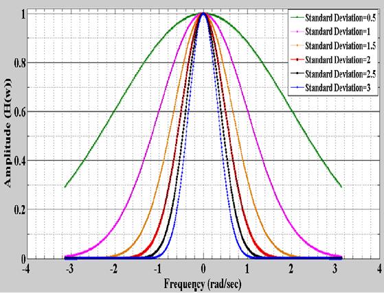
implies that the filter can be truncated at ω =± 3 σ to achieve shorter bandwidth with negligible error. For the region, 3 σ ≤ ω ≤ 3 σ the percentage error is 0.27% and the bandwidth is 24. Other properties of Gaussian filter in the frequency domain are shown in Figure 1. From the figure, it is observed that an increase in standard deviation leads to decrease in bandwidth of the filter. Figure 1 shows that standard deviation of 0.5 gives filter with the widest bandwidth while the standard deviation of 3 gives filter with the narrowest bandwidth. This implies that the bandwidth decreased with increase in standard deviation. On the other hand, smaller standard leads to higher amplitude. However, at the point where ω=0, the amplitude of the filter is independent of the standard deviation. In the time domain, the Gaussian distribution is truncated at ±3σ since the amplitude of Gaussian kernel approaches zero when the execution time becomes more than 3σ. This can be shown in the illustrations in Table4. From Table 4, it is seen that at ���� =±4 σ, the value of h(t) =0.0003 which is very close to zero. At any point when ����≥ ±5 σ, the value of h(t) is zero. This implies that the filter can be truncated at ���� =±3 σ with very negligible error and shorter execution time.

Although Gaussian filter can be truncated to enhance the speed of execution, the point of truncation must be carefully chosen to ensure minimum error. This error is calculated using the ratio of the normalized area excluded by −�������� ≤����≤ kσ region to the normalized area within ∞ ≤����≤ ∞ region. For a normalized 1-dimensional Gaussian filter the area within ∞ ≤����≤ ∞ region is unity (1).

The percentage area occupied by a region determines the accuracy and execution time of the filter if it is truncated within the region. The areas within regions in Gaussian

distribution are shown in Table 5. In Table 5, the area of a Gaussian distribution within the regions, -∞ < t < ∞ and -5 σ ≤ t≤ 5 σ are unity (1.0) each.

The area occupied by the region - σ ≤ t ≤ σ accounts for 68.27% of the total area of the distribution, the region -2σ ≤ t ≤ 2σ accounts for the 95.45% of the total area and -3σ ≤ t≤3 σ accounts for 99.73% of the of the total area. This implies that the filter can be truncated at -3σ ≤ t≤ 3σ to achieve shorter execution time with a negligible error. For the region, -3σ ≤ t≤ 3σ the percentage error is 0.27% and execution time is 1.5.

Other properties of the Gaussian filter in the time domain are shown in Figure 2. Figure 2 shows the plot of the amplitude of Gaussian filter in the time domain against time. From the figure, it is noticed that the filter with less standard deviation has the highest amplitude while a filter with higher standard deviation has the least amplitude at the point where t=0. Figure 2 also shows that filter with the highest amplitude take longer period to finish executing.

1.5. Conclusion

Based on the simulation carried out in this research, it is noticed that the standard deviation affects the performance and applications of Gaussian filter. The results show that a large standard deviation leads to long execution time and narrow frequency bandwidth of Gaussian filter. This implies that for application where speed is important, lower standard deviation is selected, but for application where a narrow frequency band is required for broad spectrum, the high standard deviation is required. It was observed that the error incurred in truncating Gaussian filter within a region in time and frequency domain is the same. However, the area enclosed by the same region is higher in the frequency domain.

IJSER

Table 3: The error and bandwidth for regions of Gaussian Filter in frequency domain for σ=0.25

(%) Bandwidth

Table 4: Effects of time on the amplitude of Gaussian filter σ =0.25 ℎ(0) = 1 595 t = 0 ℎ( 1 25) = 0 ℎ(1 25) = 0 ���� = ±5 σ ℎ( 1) = 0.0003 ℎ(1) = 0.0003 ���� = ±4 σ ℎ( 0 75) = 0 0177 ℎ(0 75) = 0 0177 ���� = ±3 σ ℎ( 0 5) = 0 2160 ℎ(0 5) = 0 2160 ���� = ±2 σ ℎ( 0 25) = 0 9679 ℎ(0 25) = 0 9679 ���� = ± σ

Table 5: The error and execution time for some regions in Gaussian filter t (σ=0.25) Region Area Region Area (%) Error (%) Execution time -∞< σ < ∞ 1 100 0.00 ∞ -5 σ ≤ t≤ 5 σ 1 100 0.00 2.5 -4σ ≤ t≤ 4 σ 0 99994 99.994 0.006 2.0 -3 σ ≤ t≤ 3 σ 0.9973 99.73 0.27 1.5 -2 σ ≤ t≤ 2σ 0.9545 95.45 4.55 1.0 - σ ≤ t≤ -σ 0 6827 68.27 31.73 0.5

Figure 1: Plot of amplitude against frequency for -π≤ ω≤ π at different standard deviation

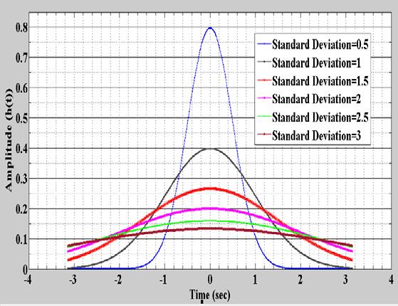
Figure 2: Plot of amplitude against time for -π≤ t≤ π at different standard deviation

References

[1] R. Van Den Boomgaard and R. Van Der Weij, “Gaussian Convolutions Numerical Approximation Based on Interpolation,” 2001.

[2] P. F. Evangelista, M. J. Embrechts, and B. K. Szymanski, “Some Properties of the Gaussian Kernel for One-Class Learning,” in Proceeding of the International Conference on Artificial Neutral Networks, 2007, vol. 4668, pp. 269–278.

[3] N. Benoudjit, A. Lendasse, J. Lee, and M. Verleysen, “Width optimization of the

Gaussian kernels in Radial Basis Function Networks,” in ESANN’2002 ProceedingsEuropean Symposium On Artificial Networks, 2002, no. April, pp. 425–432.

[4] J. Wang, H. Lu, K. N. Plataniotis, and J. Lu, “Gaussian Kernel Optimization for Pattern Classification,” Pattern Recognition, vol. 42, no. 7, pp. 1237–1247, 2009.

[5] M. Abramowitz and I. A. Stegun, Handbook of Mathematical Functions with Formulas, Graphs, and Mathematical Tables, 9th ed. New York: Dover, 1972.

IJSER