
Chapter 2
Lesson 2-1 Interpret Scatterplots
Check Your Understanding (Example 1)
Move to 68°F on the x-axis. Imagine a line of best fit. There would be about 120 water bottles sold.
Check Your Understanding (Example 2)
Because sales decrease when the temperature increases, the correlation is negative. This correlation is probably causal, so temperature is the explanatory variable and hot chocolate sales are the response variable.
Check Your Understanding (Example 3)
Taller people generally have larger feet, so a positive correlation is expected. There is causation.
Check Your Understanding (Example 4)
Point out to students that as the number of miles a car is driven increases, the balance of the loan on the car decreases. This shows a negative correlation, but there is no causation.
Check Your Understanding (Example 5)
The formula for the circumference of a circle is C =
πd. Based on the formula, as d, the diameter, increases, C, the circumference, increases. This shows a positive correlation.
Applications
1. Remind students that the terms explanatory and response are used when causation is implied. Have students offer original pairs of variables, tell how they are correlated, and determine if there seems to be causation.
2. As the number of days that have passed increases, the number of days left decreases. This is a negative correlation.
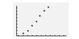
3a. As the x-values increase, the y-values increase. This scatterplot shows a positive correlation.
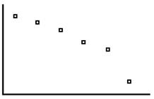
3b. As the x-values increase, the y-values decrease. This scatterplot shows a negative correlation.
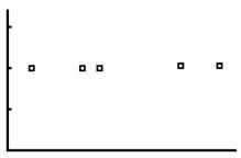
3c. As the x-values increase, the y-values do not increase or decrease. This scatterplot shows no correlation.
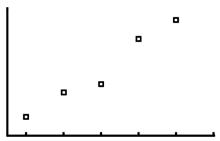
3d. As the x-values increase, the y-values decrease. This scatterplot shows a negative correlation.
3e. As the x-values increase, the y-values decrease. This scatterplot shows a negative correlation.
3f. As the x-values increase, the y-values do not increase or decrease. This scatterplot shows no correlation.
4a. In general, as the height of a student increases, the weight increases. An increase in height causes an increase in weight. Height is the explanatory variable and weight is the response variable.
4b. In general, as the number of hours studied increases, the grade increases. An increase in the number of hours studied causes an increase in grade. The number of hours studied is the explanatory variable and grade is the response variable.
4c. In general, as the number of hours worked increases, the paycheck amount increases. An increase in the number of hours worked causes an increase in paycheck amount. The number of hours worked is the explanatory variable and paycheck amount is the response variable.
4d. In general, as the number of gallons of gas consumed increases, the weight of the car decreases. An increase in the number of gallons of gas consumed causes a decrease in the weight of the car. The number of gallons of gas consumed is the explanatory variable and the weight of the car is the response variable.
5a. Let 2 represent year 2002, 3 represent year 2003, and so on. The minimum on the x-axis is 0, the maximum is 10, and the scale is 1. The minimum on the y-axis is 30,000, the maximum is 40,000, and the scale is 1,000. Enter the years in L1 and the per capita income in L2. Use the STAT PLOT feature on your graphing calculator to graph the scatterplot. The display should look similar to the one below.
5b. As the number of years increases, the per capita income increases. This scatterplot shows a positive correlation.
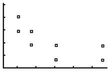
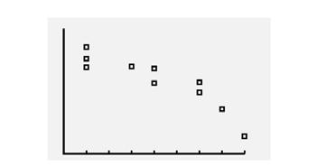
6a.The minimum on the x-axis is 0, the maximum is 1,100, and the scale is 100. The minimum on the y-axis is 0, the maximum is 5, and the scale is 1. Enter the daily dose of vitamin C in L1 and the number of colds in L2. Use the STAT PLOT feature on your graphing calculator to graph the scatterplot. The display should look similar to the one below.
7c.The minimum on the x-axis is 775, the maximum is 950, and the scale is 25. The minimum on the y-axis is 0, the maximum is 30, and the scale is 10. Enter the enrollment in L1 and the number of students on the baseball team in L2. Use the STAT PLOT feature on your graphing calculator to graph the scatterplot. The display should look similar to the one below.
6b. As the daily dose of vitamin C increases, the number of colds decreases. This is a negative correlation.
6c. The relationship seems to be casual. An increase in the daily dose of vitamin C causes a decrease in the number of colds. The daily dose of vitamin C is the explanatory variable and number of colds is the response variable.
7a. Let 6 represent year 2006, 7 represent year 2007, and so on. The minimum on the x-axis is 5, the maximum is 11, and the scale is 1. The minimum on the y-axis is 775, the maximum is 950, and the scale is 25. Enter the years in L1 and the enrollment in L2. Use the STAT PLOT feature on your graphing calculator to graph the scatterplot. The display should look similar to the one below.
7d. As the enrollment increases, the number of students on the baseball team stays the same. This scatterplot shows no correlation.
8a. As the price per song decreases, the number of downloads increases.
8b. The minimum on the x-axis is 0.3, the maximum is 1, and the scale is 0.1. The minimum on the y-axis is 1,000, the maximum is 2,250, and the scale is 250. Enter the price per song in L1 and the number of downloads in L2. Use the STAT PLOT feature on your graphing calculator to graph the scatterplot. The display should look similar to the one below.
7b. As the number of years increases, the enrollment increases. This scatterplot shows a positive correlation.
As the price per song decreases, the number of downloads increases. This scatterplot shows a negative correlation.
8c. The average of $0.59 and $0.49 is $0.54. The average of 1,877 and 1,944 is 1,910.5. The table shows the number of downloads in thousands, so multiply by 1,000: 1,910.5 × 1,000 = 1,910,500 songs.
9a. Answers vary. 9b. Answers vary. 9c. Answers vary. 9d. Answers vary.
Lesson 2-2 Linear Regression
Check Your Understanding (Example 1) Enter the ordered pairs into your calculator. Then use the statistics menu to calculate the linear regression equation. The equation of the regression line is y = –11x + 67.7.
Check Your Understanding (Example 2)
For each one-degree increase in temperature 4.44 more water bottles will be sold. So, for an increase of 2 degrees, 4.44 × 2 = 8.88, or about 9 more bottles will be sold.
Check Your Understanding (Example 3)
Substitute 83 for x in the equation of the regression line: y = 4.44(83) – 187.67 = 180.85, or about 181 water bottles. Because this is a prediction of a y-value given an x-value in the domain, this is an example of interpolation.
Check Your Understanding (Example 4)
Because –0.28 is negative, the correlation is negative. Because |–0.28| is less than 0.3, the correlation is weak.
Applications
1. The ability to make predictions is valuable in many fields. It allows you to be proactive in regard to the future, rather than just assuming you have no control over the future.
2. Graph a shows a moderate correlation that could be described by r = 0.49. Graph b is almost linear and shows a strong correlation.
3. There is no apparent causation. Both prices may have increased due to inflation over time. So, the price of a slice of pizza would not be the explanatory variable and the tuition would not be the response variable.
4a. Enter the data from the table into your calculator. Then use the statistics menu to calculate the linear regression equation. The equation of the regression line is y = 30.5x –60,384.4.
4b. The slope is the coefficient of x in the equation y = 30.5x – 60,384. The slope is 30.5.
4c. The slope is the change in y, enrollment, over the change in x, year. So the slope can be expressed as students per year as a rate.
Financial Algebra Solutions Manual
4d. Substitute 2016 for x in the equation of the regression line: y = 30.5(2016) – 60,384 = 1,101 students.
4e. Because 2016 is outside of the domain, this is an example of extrapolation.
4f. Use a graphing calculator to find the correlation coefficient. Rounded to the nearest hundredth, the correlation coefficient is 0.98.
4g. Because 0.98 is positive, the correlation is positive. Because |0.98| is greater than 0.75, the correlation is strong.
5a. 2006 + 2007 + 2008 + 2009 + 2010 = 10,040 10,040 ÷ 5 = 2008
5b. 801 + 834 + 844 + 897 + 922 = 4,298 4,298 ÷ 5 = 859.6
5c. (2008, 859.6)
5d. Substitute 2008 for x and 859.6 for y in the equation of the regression line: y = 30.5x – 60,384.4 859.6 = 30.5(2008) – 60,384.4 859.6 = 859.6
6a. Because 0.21 is positive, the correlation is positive. Because |0.21| is less than 0.3, the correlation is weak.
6b. Because –0.87 is negative, the correlation is negative. Because |–0.87| is greater than 0.75, the correlation is strong.
6c. Because 0.55 is positive, the correlation is positive. Because |0.55| is not less than 0.3 and not greater than 0.75, the correlation is moderate.
6d. Because –0.099 is negative, the correlation is negative. Because |–0.099| is less than 0.3, the correlation is weak.
6e. Because 0.99 is positive, the correlation is positive. Because |0.99| is greater than 0.75, the correlation is strong.
6f. Because –0.49 is negative, the correlation is negative. Because |–0.49| is not less than 0.3 and not greater than 0.75, the correlation is moderate.
7a. Enter the data from the table into your calculator. Then use the statistics menu to calculate the linear regression equation. The equation of the regression line is y = –1,380.57x + 2,634.90.
Chapter 2
Page 24
© 2011 Cengage Learning. All Rights Reserved. May not be scanned, copied or duplicated, or posted to a publicly accessible website, in whole or in part.
7b. The slope is the coefficient of x in the equation y = –1,380.57x + 2,634.90. The slope is –1,380.57.
7c. The slope is the change in y, number of downloads in thousands, over the change in x, price per song. So the slope can be expressed as thousands of downloads per dollar as a rate.
7d. Substitute 0.45 for x in the equation of the regression line: y = –1,380.57(0.45) + 2,634.90 = 2,013.6435 or about 2,014 thousand downloads.
7e. Because this is a prediction of a y-value given an x-value in the domain, this is an example of interpolation.
7f. Use a graphing calculator to find the correlation coefficient. Rounded to the nearest hundredth, the correlation coefficient is –0.90.
7g. Because –0.90 is negative, the correlation is negative. Because |–0.90| is greater than 0.75, the correlation is strong.
8a. Enter the data from the table into your calculator. Then use the statistics menu to calculate the linear regression equation. The equation of the regression line is y = 0.22x –0.27.
8b. The slope is the coefficient of x in the equation y = 0.22x – 0.27. The slope is 0.22.
8c. The slope is the change in y, amount of tip in dollars, over the change in x, amount of restaurant bill in dollars. So the slope can be expressed as tip dollars per restaurant bill amount as a rate.
8d. Substitute $120 for x in the equation of the regression line: y = 0.22($120) – 0.27 = $26.13 or about $26.
8e. Because $120 is outside of the domain, this is an example of extrapolation.
8f. Use a graphing calculator to find the correlation coefficient. Rounded to the nearest hundredth, the correlation coefficient is 0.75.
8g. Because 0.75 is positive, the correlation is positive. Because |0.75| is not less than 0.3 and not greater than 0.75, the correlation is moderate.
8h. In the spreadsheet, cell A2 represents x, the restaurant bill. Substitute A2 for x in the equation of the regression line: y = 0.22(A2) – 0.27. The formula for the spreadsheet is =A2*0.22–0.27.
9. A positive slope means the line is increasing, which means as x increases, y increases. If y increases as x increases, the correlation coefficient is positive. A negative slope means the line is decreasing, which means as x increases, y decreases. If y decreases as x increases, the correlation coefficient is negative.
10. The correct line of best fit is in graph c because it closely follows the trend of the data points.
11. If the points are linear, the regression line will go through every point. If the points are not linear, it may not go through any point.
Lesson 2-3 Supply and Demand
Check Your Understanding (Example 1)
Substitute x for Wholesale price and r for Retail price in the equation Markup + Wholesale price = Retail price: Markup + x = r. Subtract x from both sides of the equation: Markup = r – x
Check Your Understanding (Example 2)
Substitute 0.9 for Markup rate and x for Wholesale price in the equation Markup rate × Wholesale price = Markup: 0.9x = Markup. Then substitute x for Wholesale price and 0.9x for Markup in the equation Wholesale price + Markup = Retail price: x + 0.9x = Retail price. So Retail price = x + 0.9x or 1.9x
Check Your Understanding (Example 3)
Because $15.00 is greater than the equilibrium price of $11.00, supply will exceed demand. Suppliers will attempt to sell the widgets at a lower price.
Check Your Understanding (Example 4)
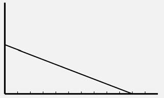
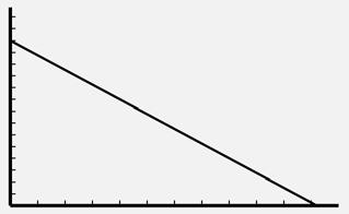
As the price increases, less quantity is demanded, so the demand function slopes downward. This is indicated by a negative slope.
Applications
1. Parrots repeat the things they hear over and over. Supply and demand is such an important concept in economics that it is constantly used by economists.
2. Markup + Wholesale price = Retail price Markup + $97 = $179.99
Markup = $82.99
© 2011 Cengage Learning. All Rights Reserved. May not be scanned, copied or duplicated, or posted to a publicly accessible website, in whole or in part.
3a. Markup + Wholesale price = Retail price
$13 + $18 = Retail price
$31 = Retail price
3b. Retail priceWholesale price Wholesale price • 100 =
3118 $18 $$ • 100 = 13 $18 $ • 100 ≈ 72%
4a. Markup + Wholesale price = Retail price
Markup + w = b
Markup = b – w
4b. Retail priceWholesale price Wholesale price • 100 = w bw • 100
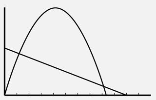
5a. The equilibrium price is the point where the supply and demand functions intersect. The equilibrium price is $1.12.
5b. Because $0.98 is less than the equilibrium price of $1.12, demand will exceed supply. Suppliers will attempt to sell the product at a higher price.
5c. y
5d. x
5e. Because $1.22 is greater than the equilibrium price of $1.12, supply will exceed demand. Suppliers will attempt to sell the product at a lower price.
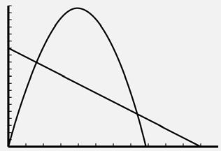
6a. The equilibrium price is the point where the supply and demand functions intersect. The equilibrium price is $35.
6b. Because $20 is less than the equilibrium price of $35, demand will exceed supply. Suppliers will attempt to sell the product at a higher price.
6c. Because $40 is greater than the equilibrium price of $35, supply will exceed demand. Suppliers will attempt to sell the product at a lower price.
6d. When the price is less than the equilibrium price, the demand will increase. So the domain that will increase the demand is p < 35.
6e. When the price is greater than the equilibrium price, the supply will increase. So the domain that will increase the supply is p > 35.
7a. The equilibrium price before the demand shift is the point where the supply function and first demand function intersect. The equilibrium price is b
7b. The equilibrium quantity before the demand shift is the point where the supply function and first demand function intersect. The equilibrium quantity is e
7c. The equilibrium price after the demand shift is the point where the supply function and second demand function intersect. The equilibrium price is a
7d. The equilibrium quantity after the demand shift is the point where the supply function and second demand function intersect. The equilibrium quantity is c.
7e. quantity demanded at price b before the shift –quantity demanded at price b after the shift = e – c
7f. A health benefit would cause a greater demand, so the demand curve would shift to the right.
8a. Enter the data from the table into your calculator. Then use the statistics menu to calculate the linear regression equation. The equation of the regression line is q = –136.08p + 2,535.79.
8b. The slope is the coefficient of p in the equation q = –136.08p + 2,535.79. The slope is –136.08. The slope is the change in q, quantity of garbage cans demanded in hundreds, over the change in p, wholesale price in dollars. So the slope can be expressed as garbage cans per dollar. For each dollar increase in price, about 136 less garbage cans are demanded.
8c. Use a graphing calculator to find the correlation coefficient. Rounded to the nearest hundredth, the correlation coefficient is –0.99. Because –0.99 is negative, the correlation is negative. Because |–0.99| is greater than 0.75, the correlation is strong.
8d. Substitute $18 for p in the equation of the regression line: q = –136.08(18) + 2,535.79 = 86.35 or about 86 hundred.
8e. Because $18 is outside of the domain, this is an example of extrapolation.
8f. $18 × 8,600 = $154,800
9a. The slope is –1,500, so for each dollar increase in the wholesale price, there will be 1,500 fewer widgets demanded.
9b. q = –1,500(20) + 90,000 = 60,000
9c. q = –1,500(21) + 90,000 = 58,500
9d. 60,000 – 58,500 = 1,500 less
9e. q = –1,500(22.50) + 90,000 = 56,250
9f. $22.50 × 56,250 = $1,265,625
9g. The markup is x + 0.5x = 1.5x. Substitute $22.50 for x: 1.5($22.50) = $33.75.
Lesson 2-4 Fixed and Variable Expenses
Check Your Understanding (Example 1)
The variable expense can be represented by
V = 6.00q, so it costs $6.00 to produce one widget.
Check Your Understanding (Example 2)
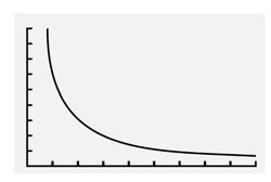
The expense for q hand warmers is 3.40q +
179,000. Divide this by q to find the average cost: + 340189000 ., q q
Check Your Understanding (Example 3)
E = 4.00(–4p + 3,000) + 78,000 = –16.00p + 12,000 + 78,000 = –16.00p + 90,000
Check Your Understanding (Example 4)
Wally’s Widget World is operating below the breakeven point. Expenses cost $140 more than what is made in revenue.
Check Your Understanding (Example 5)
Set the expense function equal to the revenue function. Then solve for q. 5.00q + 60,000 = 7.00q 60,000 = 2.00q 30,000 = q
Substitute 30,000 for q in either the expense function or the revenue function.
R = 7.00(30,000) = 210,000
The breakeven point is (30,000, 210,000).
Applications
1. Many variables are considered when making business decisions. Although economists use math models to try to predict what will happen, a change in any variable can cause a change in the expected result.
2. E = V + F, where E represents total expense, V represents variable expenses, and F represents fixed expenses. In this situation V = 4.22q Substitute 4.22q for V and 65,210 for F. The equation is E = 4.22q + 65,210.
3a. E = 1.24(1) + 142,900 = $142,901.24
3b. E = 1.24(20,000) + 142,900 = $167,700
3c. E = V + F and V = 1.24q E = 1.24q + 142,900
3d. The slope is the coefficient of q in the equation E = 1.24q + 142,900. The slope is 1.24.
3e. The slope is the change in E, expense in dollars, over the change in q, number of mini-widgets. So, the slope can be expressed as dollars per mini-widget.
4a. The fixed cost is the constant in the equation E = 4.14q + 55,789. The fixed cost is $55,789.
4b. E = 4.14(500) + 55,789 = $57,859
4c. $57,859 ÷ 500 = $155.72
4d. E = 4.14(600) + 55,789 = $58,273
4e. $58,273 ÷ 600 = $97.12
4f. The price per widget for 500 widgets is $155.72 and the price per widget for 600 widgets is $97.12, so the price decreased.
4g. E = 4.14(10,000) + 55,789 = $97,189
$97,189 ÷ 10,000 = $9.72
5. E = 5.15(3,000) + 23,500 = $38,950
$38,950 ÷ 3,000 = $12.98
6. E = 5.00q + 34,000
E = 5.00(7,000) + 34,000 = $69,000
$69,000 ÷ 7,000 = $9.86
7a. E = 2.00(–140p + 9,000) + 16,000
E = –280p + 18,000 + $16,000
E = –280p + 34,000
7b. q = –140(10) + 9,000 = $7,600
7c. E = 2.00(7,600) + 16,000 = $31,200
8. The revenue equation is R = 6.00q 3.20q + 56,000 = 6.00q
56,000 = 2.8q
20,000 = q
9. The revenue equation is R = 20.00q
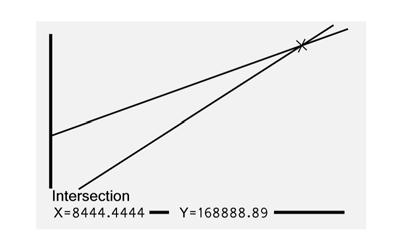
11.00q + 76,000 = 20.00q 76,000 = 9.00q 84,444 = q
10. Enter the expense equation in Y1 and the revenue equation in Y2. Use the ZoomFit feature to view the graph. Then use the Intersect feature to find the intersection.
13b.
The graph shows the same solution as solving the equations.
11a. $4.98 – $4.55 = $0.43
11b. The revenue equation is R = 8.00q
4.55q + 69,000 = 8.00q 69,000 = 3.45q 20,000 = q
Substitute 20,000 for q in the expense equation.
E = 4.55(20,000) + 69,000 = $160,000
The breakeven point is (20,000, $160,000).
11c. The revenue equation is R = 8.50q
4.98q + 69,000 = 8.50q 69,000 = 3.52q 19,602 = q
Substitute 19,602 for q in the expense equation.
E = 4.98(19,602) + 69,000 = $166,618
The breakeven point is (19,602, $166,618).
12a. The breakeven point is the place where the revenue and expense equations intersect, (A, W).
12b. There is a loss because expenses are greater than revenue at any quantity less than A.
12c. There is a profit because revenue is greater than expenses at any quantity greater than A
12d. If no items are sold, the company still has to pay Z dollars for the fixed expenses.
13a. The expense for q Nokee’s is 6.21q + 125,000. Divide this by q to find the average cost: + 621125000 ., q q
13c. + 621125000 ., q q is not in the form of y = mx + b, so it is not linear.
13d. When dividing by a greater amount, the quotient is smaller. So when q increases, the average expense function decreases.
13e. + 6211125000 1 .(), () = $125,006.21
13f. + 621100000125000 100000 .(,), (,) = $7.46
14. The expense for W products is 10.75W + N Divide this by W to find the average cost: + 1075WN W . Simplify: 10.75 + N W
Lesson 2-5 Graphs of Expense and Revenue Functions
Check Your Understanding (Example 1)
Students must first create the expense function in terms of q; E = 5q + 20,000. Then, substitute the expression for q given in the problem statement. This yields an expense function in terms of the price p
E = 5(–200p + 40,000) + 20,000
E = –1,000p + 200,000 + 20,000
E = –1,000p + 220,000
The horizontal intercept is 220. This can help you select viewing window values of 0 to 250 with a scale of 50. The vertical intercept is 220,000. Set the viewing window: Xmin = 0, Xmax = 15, Xscl = 1, Ymin = 200,000, Ymax = 250,000, Yscal = 1,000.
Check Your Understanding (Example 2)
Substitute 25 for p
2
R = –500(25) + 30,000(25) = $437,500
Check Your Understanding (Example 3)
Because $28 is closer to $30 than $40, it will yield a higher point on the parabola.
Check Your Understanding (Example 4)
At both prices, revenue is less than expenses. The price of $7.50 is too low for the incoming revenue to make up for the outgoing expenses. The price of $61 may be too high for consumers and would decrease the demand for the product. Therefore, with fewer items being sold, the revenue will be less.
Applications
1. Emerson cautions to be aware of the fact that the expenses involved in making revenue are often more than the revenue itself.
2a. E = V + F and V = 1.00q
E = 1.00q + 1,500
2b. E = 1.00(–1,000p + 8,500) + 1,500
E = –1,000p + 8,500 + 1,500
E = –1,000p + 10,000
2c. The intercepts are (0, 10,000) and (10, 0), so the viewing window can be set from 0 to 12 with a scale of 1 for the horizontal axis and 0 to 12,000 for the vertical axis with a scale of 100.
2d.
2e. R = pq
R = p(–1,000p + 8,500)
2 R = –1,000p + 8,500p
2f. 2 b a = 8500 21000 , ( , ) = 8500 2000 , , = 4.25
R = –1,000(4.25)2 + 8,500(4.25) = $18,062.50 The maximum revenue of $18,062.50 is achieved when the price is $4.25.
2g. Enter the expense equation in Y1 and the revenue equation in Y2. Use the ZoomFit feature to view the graph. Then use the Intersect feature to find the intersection.
The graphs intersect at (1.21, 8,794.36) and (8.29, 1,705.64). The breakeven prices are $1.21 and $8.29.
3a. E = V + F and V = 5q
E = 5q + 40,000
3b. E = 5(–500p + 20,000) + 40,000
E = –2,500p + 100,000 + 40,000
E = –2,500p + 140,000
3c. The intercepts are (0, 140,000) and (56, 0), so the viewing window can be set from 0 to 60 with a scale of 5 for the horizontal axis and 0 to 150,000 for the vertical axis with a scale of 10,000.
3d.
3e. R = pq
R = p(–500p + 20,000)
R = –500p 2 + 20,000p
3f. 2 b a = 20000 2500 , () = 20000 1000 , , = 20
R = –500(20)2 + 20,000(20) = $200,000
The maximum revenue of $200,000 is achieved when the price is $20.00.
Lesson 2-6 Breakeven Analysis
Check Your Understanding (Example 1)
E = R
–2,000p + 125,000 = –600p 2 + 18,000p 600p 2 – 20,000p + 125,000 = 0
Substitute 600 for a, –20,000 for b and 125,000 for c in the quadratic formula. Use p instead of x
3g. Enter the expense equation in Y1 and the revenue equation in Y2. Use the ZoomFit feature to view the graph. Then use the Intersect feature to find the intersection.
The graphs intersect at (7.46, 121,354.02) and (37.54, 46,145.98). The breakeven prices are $7.46 and $37.54.
= −±− 2 4
bbac a p = −−+−− 2 20000200004600125000 2600 ( , )( , )( )( , ) () = $25
p =
2 20000200004600125000 2600 ( , )( , )( )( , ) ()
Enter the expense equation in Y1 and the revenue equation in Y2. Use the ZoomFit feature to view the graph. Then use the Intersect feature to find the intersection. The breakeven prices are $25 and $8.33.
Extend Your Understanding (Example 1)
The actual breakeven values from Example 1 have non-terminating decimal parts, so using the rounded values will not yield exact expense and revenue values. The expense and revenue values are approximately equal when p = 8.08 and p = 58.92.
Check Your Understanding (Example 2)
The error could have been improved by using more accurate prices with more decimal places in the calculations. But, for this purpose, it is acceptable to round to the nearest cent.
Check Your Understanding (Example 3)
Because the value in B11 is the same as the value in B7, the formula in B11 is =B7. The value in B12 is the difference between B and V. Therefore, the formula in B12 is =(B8–B3). The value in B13 is the negative value in B4. The formula in B13 is =–B4.
Applications
1. Warren Buffet speaks to the need to be knowledgeable in order to minimize or eliminate risk. With the knowledge of the prices and subsequent revenue at breakeven points, the risk of putting a product on the market can be minimized.
2. Divide the expense by the number of items: $10,000,000 ÷ 500,000 = $20.
3a. Divide the expense by the number of items: W ÷ G = W G
3b. “Twice as many kits” means 2G and “80% of the cost” means 0.8W. So the expression is 08 2 . W G .
4a. 1,250q + 800,000 = 2,600,000 1,250q = 1,800,000
q = 1,440 necklaces
4b. 1,250q + 800,000 = 3,500,000
1,250q = 2,700,000
q = 2,160 necklaces
2,160 is greater than 1,440, so the quantity demanded increased.
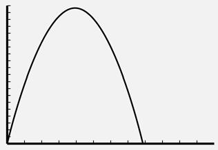
5. Answers vary. Sample graph is shown.
6. Answers vary. Sample graph is shown.
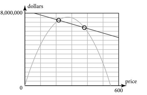
7b. –19,000p + 6,300,000 = –1,000p 2 + 155,000p 1,000p 2 – 174,000p + 6,300,000 = 0 p = $51.38 and p = $122.62
7c. When p = $51.38, E = –19,000(51.38) + 6,300,000 = $5,323,780.00 and R = –1,000(51.38)2 + 155,000(51.38) = $5,232,995.60. When p = $122.62, E = –19,000(122.62) + 6,300,000 = $3,970,220.00 and R = –1,000(122.62)2 + 155,000(122.62) = $3,970,435.60.
 7a.
7a.
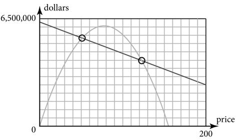
8b. –5,000p + 8,300,000 = –100p 2 + 55,500p 100p 2 – 60,500p + 8,300,000 = 0 p = $210.27 and p = $394.73
8c. When p = $210.27, E = –5,000(210.27) + 8,300,000 = $7,248,650.00 and R = –100(210.27)2 + 55,500(210.27) = $7,248,637.71. When p = $394.73, E = –5,000(394.73) + 8,300,000 = $6,326,350.00 and R = –100(394.73)2 + 55,500(394.73) = $6,326,337.71.
9a. Find the maximum point on the graph of R = –18p 2 + 800p. If the bookcase is set at $22.22 then the maximum revenue would be approximately $8,888.89.
9b.
9c. –200p + 10,000 = –18p 2 + 800p 18p 2 – 1,000p + 10,000 = 0 p = $13.08 and p = $42.48
9d. When p = $13.08, E = –200(13.08) + 10,000 = $7,384.00 and R = –18(13.08)2 + 800(13.08) = $7,384.44. When p = $42.48, E = –200(42.48) + 10,000 = $1,504.00 and R = –18(42.48)2 + 800(42.48) = $1,502.09.
10a. Find the maximum point on the graph of R = –32p 2 + 1,200p. The maximum revenue would be reached when the price is set at $18.75.
10b. Find the maximum point on the graph of R = –32p 2 + 1,200p. The maximum revenue at price $18.75 is $11,250.00.
10c.
10d. –300p + 13,000 = –32p 2 + 1,200p 32p 2 – 1,500p + 13,000 = 0 p = $11.48 and p = $35.40
10e. When p = $11.48, E = –300(11.48) + 13,000 = $9,556.00 and R = –32(11.48)2 + 1,200(11.48) = $9,558.71. When p = $35.40, E = –300(35.40) + 13,000 = $2,380.00 and R = –32(35.40)2 + 1,200(35.40) = $2,378.88.
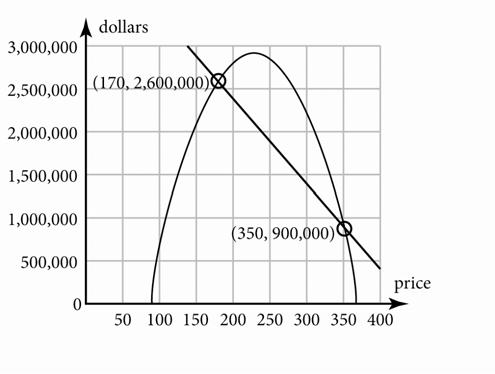
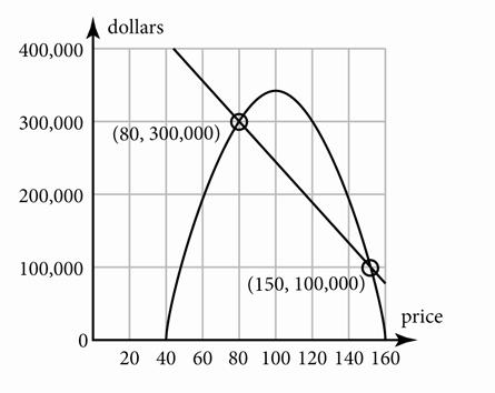
11. Find the maximum point, or vertex on the graph. The price is the horizontal scale. The scale for the price is $20. The maximum profit is reached at the price of $60.
12. Find the points on the graph that intersect. The price at these points is $40 and $80.
13. List any price between the breakeven point prices of $40 and $80. For example, $45 and $50.
14. List any price below the breakeven point price of $40 and above the breakeven point price of $80. For example, $35 and $150.
Lesson 2-7 The Profit Equation
Check Your Understanding (Example 1)
P = R – E
P = –350p 2 + 18,000p –(–1,500p + 199,000)
P = –350p 2 + 18,000p + 1,500p – 199,000
P = –350p 2 + 19,500p – 199,000
Check Your Understanding (Example 2)
The graph is shown in Example 2. The two points where the profit function intersects the horizontal axis indicate item prices at which no profit is made. These prices are $8.07 and $58.93.
Check Your Understanding (Example 3)
No; the greatest difference between revenue and expense does not depend on the maximum revenue.
Check Your Understanding (Example 4)
Identify the values of a, b, and c: a = –350, b = 19,500, and c = –199,000. Find the x-intercept of the axis of symmetry by using the expression
2
b a = 19500 2350 , () = 19500 700 , = 27.86
Substitute 27.86 for p in the profit equation. 2 P = –350(27.86) + 19,500(27.86) – 199,000 = $72,607.14.
Applications
1. A person would lose money when the expense is greater than the revenue. A true profit equation is found in the first quadrant and is the difference between the revenue and the expense. If the expense is greater than the revenue, then there is no profit. Therefore, no one would lose money if they take (make) a profit!
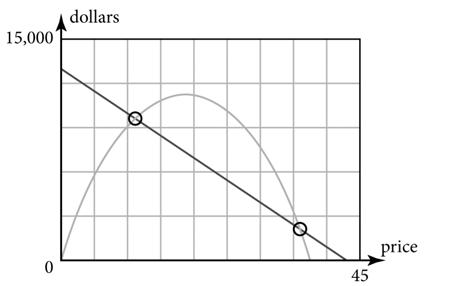
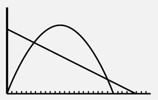
2. The expenses are fixed for this product. Regardless of price, the expenses are $500,000. A profit is made when the price is set approximately between $20 and $60.
3. This situation is similar to that examined in Skills and Strategies. Expenses decrease as the price of the item increases. Profit is made when the price is set approximately between $13 and $70.
4. The expenses are greater than the revenue at all possible prices. No profit can be made from the sale of this item.
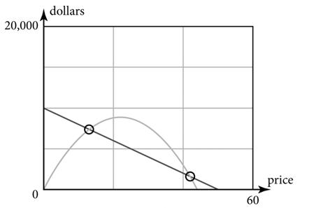
5. This situation is similar to that examined in Skills and Strategies. Expenses decrease as the price of the item increases. Profit is made when the price is set approximately between $7 and $18.
6. P = R – E
P = –2,170p 2 + 87,000p – (–20,000p + 90,000)
2 P = –2,170p + 87,000p + 20,000p – 90,000
2 P = –2,170p + 107,000p – 90,000
7. P = R – E
P = –720p 2 + 19,000p – (–6,500p + 300,000)
P = –720p 2 + 19,000p + 6,500p – 300,000
P = –720p 2 + 25,500p – 300,000
8. P = R – E
P = –330p 2 + 9,000p – (–2,500p + 80,000)
P = –330p 2 + 9,000p + 2,500p – 80,000
P = –330p 2 + 11,500p – 80,000
9. P = R – E
P = –1,450p 2 + 55,000p – (–12,500p + 78,000)
P = –1,450p 2 + 55,000p + 12,500p – 78,000
P = –1,450p 2 + 67,500p – 78,000
10. Approximately $26; it appears to have the greatest positive vertical distance from the revenue to the expense function.
11a. In Exercise 7 the expense is always greater than the revenue.
11b. If expenses are always greater than the revenue, the profit parabola will lie entirely below the horizontal axis.
12a. 2 b a = 12400 2400 , () = 12400 800 , = $15.50
P = –400(15.50)2 + 12,400(15.50) – 50,000 = $46,100
At the price of $15.50, the maximum profit would be $46,100.
12b. 2 b a = 8800 2370 , () = 8800 740 , = $11.89
P = –370(11.89)2 + 8,800(11.89) – 25,000 = $27,324.32
At the price of $11.89, the maximum profit would be $27,324.32.
12c. 2 b a = 88800 2170 , () = 88800 340 , = $261.18
P = –170(261.18)2 + 88,800(261.18) – 55,000 = $11,541,235.29
At the price of $261.18, the maximum profit would be $11,541,235.29.
13a. P = R – E
P = –100p 2 + 20,000p – (–1,850p + 800,000)
P = –100p 2 + 20,000p + 1,850p – 800,000
P = –100p 2 + 21,850p – 800,000
13b. 2 b a = 21850 2100 , () = 21850 200 , = $109.25
13c. P = –100(109.25)2 + 21,850(109.25) – 800,000 = $393,556.25
14a. P = R – E
P = –185p 2 + 9,000p – (–450p + 90,000)
P = –185p 2 + 9,000p + 450p – 90,000
P = –185p 2 + 9,450p – 90,000
14b. 2 b a = 9450 2185 , () = 9450 370 , = $25.54
14c. P = –185(25.54)2 + 9,450(25.54) – 90,000 = $30,679.05
15a. P = R – E
P = –225p 2 + 7,200p – (–250p + 50,000)
P = –225p 2 + 7,200p + 250p – 50,000
P = –225p 2 + 7,450p – 50,000
15b.
2 b a = 7200 2225 , () = 7450 450 , = $16.56
15c. P = –225(16.56)2 + 7,450(16.56) – 50,000 = $11,669.44
16a. P = R – E
P = –275p 2 + 6,500p – (–300p + 32,000)
P = –275p 2 + 6,500p + 300p – 32,000
P = –275p 2 + 6,800p – 32,000
16b. 2 b a = 6800 2275 , () = 6800 550 , = $12.36
16c. P = –275(12.36)2 + 6,800(12.36) – 32,000 = $10,036.36
Lesson 2-8 Mathematically Modeling a Business
Check Your Understanding (Example 1)
Substitute 80p + 100,000 for q in the equation
E = 50q + 80,000.
E = 50(80p + 100,000) + 80,000
E = 4,000p + 5,000,000 + 80,000
E = 4,000p + 5,080,000
Substitute 42 for p
E = 4,000(42) + 5,080,000
E = 168,000 + 5,080,000
E = $5,248,000
Extend Your Understanding (Example 1)
Once the value of z is known, then y can be calculated. With y calculated, then x can be determined. Once x is determined, it is substituted into the first equation, and A can be evaluated.
Check Your Understanding (Example 2)
The maximum point on the profit function is (40, 380,000). The expense at a price of $40 is $420,000 and the revenue at a price of $40 is $800,000. Subtract the expense from the revenue: $800,000 – $420,000 = $380,000.
Applications
1. Models simulate reality but they themselves are not reality. There are a fixed number of variables that are used in models. In reality, there are many more variables that contribute to the outcome of a situation. So, while models can be wrong, they can still be useful.
2a. (D, B) is the first intersection of the expense function and the revenue function, so this is the first breakeven point.
2b. (E, A) is the vertex of the parabola, so this is the maximum revenue point.
2c. (F, C) is the second intersection of the expense function and the revenue function, so this is the second breakeven point.
2d. (G, 0) is on the revenue function and intersects the horizontal axis, so this is a price at which no revenue is made.
2e. (H, 0) is on the expense function and intersects the horizontal axis, so this is a price at which there are no expenses.
2f. The maximum profit occurs where there is the greatest vertical difference between the revenue and expense functions. It appears that this might happen at an x value slightly to the left of E
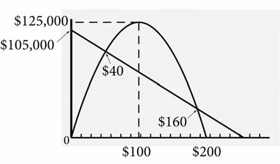
3. The revenue function should reach a maximum height of $125,000. The expense function and revenue function should intersect at the price of $40 and $160. The revenue function should intersect the horizontal axis at $200. The expense function should intersect the vertical axis at $105,000.
4. As the price of a product increases, the demand decreases.
5. As the price of a product increases, the demand decreases, so the demand function will decrease from left to right. Therefore the slope is negative.

6. The minimum on the x-axis is 10, the maximum is 18, and the scale is 2. The minimum on the y-axis is 5,000, the maximum is 10,000, and the scale is 1,000. Enter the p coordinates in L1 and the q coordinates in L2. Use the STAT PLOT feature on your graphing calculator to graph the scatterplot. The display should look similar to the one below.
14b. Evaluate the expense function when p = 0. –2,592.49(0) + 112,113.55 = 112,113.55
Since the expense function will intersect the vertical axis at about 112,113.55, a maximum vertical-axis value of 130,000 is reasonable.
14c.
The scatterplot has a linear form.
7. Enter the ordered pairs into your calculator. Then use the statistics menu to calculate the linear regression equation. The equation of the regression line is q = –423.61p + 14,315.94.
8. Based on the correlation coefficient of –0.92, the linear regression line is a good predictor.
9. r = –0.92; This is a significant correlation because the coefficient is close to –1.
10. E = V + F
E = 6.12q + 24,500
11. The revenue equation is R = pq.
12. R = pq
R = p(–423.61p + 14,315.94)
R = –423.61p 2 + 14,315.94p
13. E = 6.12q + 24,500
E = 6.12(–423.61p + 14,315.94) + 24,500
E = –2,592.49p + 87,613.55 + 24,500
E = –2,592.49p + 112,113.55
14a. Set the expense function equal to 0. 0 = –2,592.49p + 112,113.55
–112,113.55 = –2,592.49p
43.25 ≈ p
Since the expense function will intersect the horizontal axis at about 43.25, a maximum horizontal-axis value of 50 is reasonable.
15. 2 b a = 1431594 242361 ,. ( ) = 1431594 84722 ,. = 16.90
R = –423.61(16.90)2 + 14,315.94(16.90) = 120,952.13
The coordinates of the maximum point are (16.90, 120,952.13).
16. Graph the expense and revenue functions on a graphing calculator. Use the Intersect feature. The breakeven points are (8.40, 90,343.87) and (31.52, 30,403.76).
17. P = R – E
P = –423.61p 2 + 14,315.94p – (–2,592.49p + 112,113.55)
P = –423.61p 2 + 14,315.94p + 2,592.49p –
112,113.55
P = –423.61p 2 + 16,908.43p – 112,113.55
18. Enter the profit equation P = –423.61p 2 + 16,908.43p – 112,113.55 into a graphing calculator. The maximum profit is the vertex of the parabola. Use the maximum feature on your calculator to find the maximum. The coordinate of the maximum is (19.96, 56,611.81). The profit is maximized at a price of $19.96.

Assessment
Really? Really! Revisited
1. Look at the first section of bars, which is condition 6. The year 2008 is the green bar. The green bar is about halfway between $0 and $2,000. So the value for the 1958 Villager in a condition of 6 in 2008 is about $1,000.
2. Look at the fifth section of bars, which is condition 2. The year 2008 is the green bar. The green bar is about up to the $14,000 line on the bar graph. So the value for the 1958 Villager in a condition of 2 in 2008 is about $14,000.
3. Subtract the value of a 1958 Villager in a condition of 6 in 2008 from a 1958 Villager in a condition of 2 in 2008: $14,000 – $1,000 = $13,000.
19a. To start this business, make the number of Toejacks that maximizes the profit: 5,861.
19b. Each Toejack should be sold at the price that maximizes the profit: $19.96.
19c. There are two prices that cause the revenue and expense to be equal. The first breakeven price is $8.40.
19d. There are two prices that cause the revenue and expense to be equal. The second breakeven price is $31.52.
19e. At the selling price of $19.96, the revenue is –423.61(19.96)2 + 14,315.94(19.96) = $116,979.26.
19f. At the selling price of $19.96, the expense is –2,592.49(19.96) + 112,113.55 = $60,367.45.
19g. The profit is the revenue minus the expense: $116,979.26 – $60,367.45 = $56,611.81.
20. To start the business, there has to be enough money for the expenses. The expenses are $60,367.45. Divide the expenses by the price per stock: $60,367.45 ÷ $5 = 12,073.49. Round up to the next whole stock to ensure that there is enough money for the expenses. So there should be 12,074 shares sold.
4. The value for the 1958 Villager in a condition of 2 in 1999 is about $7,000. The value for the 1958 Villager in a condition of 2 in 2008 is about $14,000. Subtract the value of a 1958 Villager in a condition of 2 in 1999 from a 1958 Villager in a condition of 2 in 2008: $14,000 – $7,000 = $7,000.
Applications
1a. As the x-values increase, the y-values decrease. This scatterplot shows a negative correlation.
1b. As the x-values increase, the y-values decrease. This scatterplot shows a negative correlation.
1c. As the x-values increase, the y-values do not increase or decrease. This scatterplot shows no correlation.
2a. In general, as the number of hours spent reading increases, the number of pages read increases. An increase in the number of hours causes an increase in the number of pages read. The number of hours is the explanatory variable and number of pages read is the response variable.
2b. In general, as the number of minutes exercised increases, the number of calories burned increases. An increase in the number of minutes exercised causes an increase in the number of calories burned. The number of minutes exercised is the explanatory variable and the number of calories burned is the response variable.
2c. In general, as the amount of a paycheck increases, the amount paid in income taxes increases. An increase in the amount of a paycheck causes an increase in the amount paid in income taxes. The amount of a paycheck is the explanatory variable and the amount paid in income taxes is the response variable.
2d. In general, as the number of pounds of hamburger increases, the number of people that can be fed increases. An increase in the number of pounds of hamburger causes an increase in the number of people that can be fed. The number of pounds of hamburger is the explanatory variable and the number of people that can be fed is the response variable.
3. A line of best fit is a straight line. Graph b does not show a straight line, so this graph does not show a line of best fit.
4a. Because 0.17 is positive, the correlation is positive. Because |0.17| is less than 0.3, the correlation is weak.
4b. Because –0.62 is negative, the correlation is negative. Because |–0.62| is not less than 0.3 and not greater than 0.75, the correlation is moderate.
4c. Because –0.88 is negative, the correlation is negative. Because |–0.88| is greater than 0.75, the correlation is strong.
4d. Because 0.33 is positive, the correlation is positive. Because |0.33| is not less than 0.3 and not greater than 0.75, the correlation is moderate.
4e. Because 0.49 is positive, the correlation is positive. Because |0.49| is not less than 0.3 and not greater than 0.75, the correlation is moderate.
4f. Because –0.25 is negative, the correlation is negative. Because |–0.25| is less than 0.3, the correlation is weak.
4g. Because 0.91 is positive, the correlation is positive. Because |0.91| is greater than 0.75, the correlation is strong.
5a. The equilibrium price is the point where the supply and demand functions intersect. The equilibrium price is $11.49.
5b. Because $7.99 is less than the equilibrium price of $11.49, demand will exceed supply. Suppliers will attempt to sell the product at a higher price.
5c. Find the place on the demand curve where the price is $7.99. There are 1,000 game controllers demanded at a price of $7.99.
5d. Find the place on the supply curve where the price is $7.99. There are 250 game controllers supplied at a price of $7.99.
5e. Because $12.99 is greater than the equilibrium price of $11.49, supply will exceed demand. Suppliers will attempt to sell the product at a lower price.
6a. E = V + F, where E represents total expense, V represents variable expenses, and F represents fixed expenses. In this situation V = 2q. Substitute 2q for V and 500,000 for F. The equation is E = 2q + 500,000.
6b. E = 2q + 500,000
E = 2(–300p + 10,000) + 500,000
E = –600p + 20,000 + 500,000
E = –600p + 520,000
6c. q = –300p + 10,000
q = –300(20) + 10,000
q = –6,000 + 10,000
q = 4,000
6d. q = –300p + 10,000
q = –300(25) + 10,000
q = –7,500 + 10,000
q = 2,500
When the price is set at $25 per item, the demand for the item will be 2,500.
6e. E = 2q + 500,000
E = 2(1,000) + 500,000
E = 2,000 + 500,000
E = 502,000
It cost $502,000 to produce 1,000 widgets.
6f. E = –600p + 520,000
E = –600(15) + 520,000
E = –9,000 + 520,000
E = 511,000
It would cost $511,000 to produce widgets that sell for $15 each.
© 2011 Cengage Learning. All Rights Reserved. May not be scanned, copied or duplicated, or posted to a publicly accessible website, in whole or in part.
7a. Enter the expense equation in Y1 and the revenue equation in Y2. Use the viewing window given.
12. The minimum on the x-axis is 275, the maximum is 550, and the scale is 25. The minimum on the y-axis is 2,500, the maximum is 10,500, and the scale is 500. Enter the p coordinates in L1 and the q coordinates in L2. Use the STAT PLOT feature on your graphing calculator to graph the scatterplot. The display should look similar to the one below.
7b. Use the Intersect feature to find the intersection. The first point where the two graphs intersect is at (6, 42,026), so x = 6 and y = 42,026.
7c. When the price is set at approximately $6, both the revenue and the expense will be approximately $42,026.
8a. R = pq
R = p(–900p + 120,000)
R = –900p 2 + 120,000p
8b. R = pq
R = p(–88,000p + 234,000,000)
R = –88,000p 2 + 234,000,000p
9a. P = R – E
P = –600p 2 + 25,000p – (–3,000p + 250,000)
P = –600p 2 + 25,000p + 3,000p – 250,000
P = –600p 2 + 28,000p – 250,000
9b. 2 b a = 28000 2600 , () = 28000 1200 , , = $23.33
P = –600(23.33)2 + 28,000(23.33) – 250,000 = $76,666.66
The maximum profit price is approximately $23.33. At that price, the maximum profit is approximately $76,666.66.
10. As the price of the eyePOD increases, the demand decreases.
11. As the price of the eyePOD increases, the demand decreases, so the demand function will decrease from left to right. Therefore the slope is negative.
13. Enter the ordered pairs into your calculator. Then use the statistics menu to calculate the linear regression equation. The correlation coefficient is 0.98. Because 0.98 is positive, the correlation is positive. Because |0.98| is greater than 0.75, the correlation is strong.
14. Enter the ordered pairs into your calculator. Then use the statistics menu to calculate the linear regression equation. The equation of the regression line is q = –30.74p + 19,330.
15. E = V + F
E = 150q + 160,000
16. The revenue equation is R = pq.
17. R = pq
R = p(–30.74p + 19,330)
R = –30.74p 2 + 19,330p

18. E = 150q + 160,000
E = 150(–30.74p + 19,330) + 160,000
E = –4,611p + 2,899,500 + 160,000
E = –4,611p + 3,059,500
19a. Set the expense function equal to 0.
0 = –4,611p + 3,059,500
–3,059,500 = –4,611p
663.52 ≈ p
Since the expense function will intersect the horizontal axis at about 663.52, a maximum horizontal-axis value of 700 is reasonable.
19b. Evaluate the expense function when p = 0. –4,611(0) + 3,059,500 = 3,059,500
Since the expense function will intersect the vertical axis at about 3,059,500, a maximum vertical-axis value of 3,100,000 is reasonable.
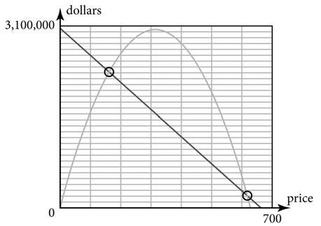
19c.
20. 2 b a = 19330 23074 , ( ) = 19330 6148 , = $314.41
R = –30.74(314.41)2 + 19,330(314.41) = $3,038,784.16
The coordinates of the maximum point are (314.41, 3,038,784.16).
21. Graph the expense and revenue functions on a graphing calculator. Use the Intersect feature. The breakeven points are (8.40, 90,336.63) and (31.52, 30,398.27).
22. P = R – E
P = –30.74p 2 + 19,330p – (–4,611p + 3,059,500)
P = –30.74p 2 + 19,330p + 4,611p – 3,059,500
P = –30.74p 2 + 23,941p – 3,059,500
23. Enter the profit equation P = –30.74p 2 + 23,941p – 3,059,500 into a graphing calculator. The maximum profit is the vertex of the parabola. Use the maximum feature on your calculator to find the maximum. The coordinate of the maximum is (389.41, 1,601,946.66). The profit is maximized at a price of $389.41.
24a. To start this business, make the number of eyePODs that maximizes the profit: 7,360.
24b. Each eyePOD should be sold at the price that maximizes the profit: $389.41.
24c. There are two prices that cause the revenue and expenses to be equal. The first breakeven price is $161.13.
24d. There are two prices that cause the revenue and expenses to be equal. The second breakeven price is $617.69.
24e. At the selling price of $379.41, the revenue is –30.74(389.41)2 + 19,330(389.41) = $2,865,877.15.
24f. At the selling price of $389.41, the expense is –4,611(389.41) + 3,059,500 = $1,263,930.49.
24g. The profit is the revenue minus the expense: $2,865,877.15 – $1,263,930.49 = $1,601,946.66.
25. To start the business, there has to be enough money for the expenses. The expenses are $1,263,930.49. Divide the expenses by the price per stock: $1,263,930.49 ÷ $10 = 126,393.05. Round up to the next whole stock to ensure that there is enough money for the expenses. So there should be 126,394 shares sold.
© 2011 Cengage Learning. All Rights Reserved. May not be scanned, copied or duplicated, or posted to a publicly accessible website, in whole or in part.