Introductory statistics 9th edition mann solutions manual

Chapter 3

Numerical Descriptive Measures

Section 3.1

3.1 For a data set with an odd number of observations, first we rank the data set in increasing (or decreasing) order and then find the value of the middle term. This value is the median. For a data set with an even number of observations, first we rank the data set in increasing (or decreasing) order and then find the average of the two middle terms. The average gives the median.

3.2 A few values that are either very small or very large relative to the majority of the values in a data set are called outliers or extreme values. Suppose the exam scores for seven students are 73, 82, 95, 79, 22, 86, and 91. Then, 22 is an outlier because this value is very small compared to the other values. The median is a better measure of central tendency as compared to the mean for a data set that contains an outlier because the mean is affected much more by outliers than is the median.

3.3 Suppose the exam scores for seven students are 73, 82, 95, 79, 22, 86, and 91 points. Then, Mean = (73 + 82 + 95 + 79 + 22 + 86 + 91)/7 = 75.43 points. If we drop the outlier (22), Mean = (73 + 82 + 95 + 79 + 86 + 91)/6 = 84.33 points. This shows how an outlier can affect the value of the mean.

3.4 All five measures of central tendency (mean, median, mode, trimmed mean, and weighted mean) can be calculated for quantitative data. Note that the mode may or may not exist for a data set. However, only the mode (if it exists) can be found for a qualitative data set. Examples given in Sections 3.1.1, 3.1.2, and 3.1.3 of the text show these cases.

3.5 The mode can assume more than one value for a data set. Examples 3–8 and 3–9 of the text present such cases.

3.6 A quantitative data set will definitely have a mean and a median but it may or may not have a mode. Example 3–7 of the text presents a data set that has no mode.

3.7 For a symmetric histogram (with one peak), the values of the mean, median, and mode are all roughly equal. Figure 3.2 of the text shows this case. For a histogram that is skewed to the right, the value of the mode is the smallest and the value of the mean is the largest. The median lies between the mode and the mean. Such a case is presented in Figure 3.3 of the text. For a histogram that is skewed to the left, the value of the mean is the smallest, the value of the mode is the largest, and the value of the median lies between the mean and the mode. Figure 3.4 of the text exhibits this case.

3.8 The median is the best measure to summarize this data set since it is not influenced by the skew or outliers.

3.9 Σx = 5 + (–7) + 2 + 0 + (–9) + 16 +10 + 7 = 24

μ = (Σx)/N = 24/8 = 3

Median = value of the 4.5th term in ranked data = (2 + 5)/2 = 3.50

This data set has no mode.

3.10 x = (Σx)/n = $158,542/10 = $15,854.20

Median = average of the 5th and 6th terms in ranked data set = $14,539.50. There is no mode since all values occur exactly once.

3.11 x = (Σx)/N = 3,169/12 = 264.08

Median = average of the 6th and 7th terms in ranked data set = 262. There is no mode since all values occur exactly once.

3.12 a. x = (Σx)/n = 463/20 = 23.15 years

Median = average of the 10th and 11th terms in ranked data set = 21 years. The mode is 5 and 27 since both values occur twice and all others just once

b. For the 10% trimmed mean, we must remove 0.10(20) = 2 values from each end of the ranked data set. So, we discard 3, 5, 51, and 59 and average the remaining 16 values to get 345/16 = 21.5625 years.

3.13 a. x = (Σx)/n = 4298/10 = 429.80 thousands of dollars.

Median = average of the 5th and 6th terms in ranked data set = 103.5 thousand dollars

b. There is no mode because all values occur exactly once.

c. For the 10% trimmed mean, we must remove 0.10(10) = 1 value from each end of the ranked data set and then average the remaining 8 values to get 992/8 = 124 thousand dollars.

d. Median and trimmed mean are good measures to use where there is an outlier.

3.14 a. x = (Σx)/n = 19,167/20 = 958.35 dollars

Median = average of the 10th and 11th terms in ranked data set = 990 dollars.

b. For the 20% trimmed mean, we must remove 0.20(20) = 4 values from each end of the ranked data set and average the remaining 16 values to get 15,466/16 = 966.63 dollars.

3.15 a. x = (Σx)/n = 2,440/10 = 244 thousand dollars.

Median = average of the 5th and 6th terms in ranked data set = 235 thousand dollars.

b. For the 10% trimmed mean, we must remove 0.10(10) = 1 value from each end of the ranked data set and average the remaining 8 values to get 1,927/8 = 240.875 thousand dollars.

3.16 a. x = (Σx)/n = 1,113/20 = 55.65 thousand dollars

Median = average of the 10th and 11th terms in ranked data set = 57.5 thousand dollars. The mode is 64 because it occurs twice and all other values occur just once.

b. For the 15% trimmed mean, we must remove 0.15(20) = 3 values from each end of the ranked data set and average the remaining 14 values to get 779/14 = 55.64 thousand dollars

3.17 a. x = (Σx)/n = 597/20 = 29.85 patients

Median = average of the 10th and 11th terms in ranked data set = 29.5 patients

Each of 24, 26, 37, 38 are modes because they each occur twice and all other values exactly once.

b. For the 15% trimmed mean, we must remove 0.15(20) = 3 values from each end of the ranked data set and average the remaining 14 values to get 418/14 = 29.86 patients.

3.18 a. x = (Σx)/n = 2,651/20 = 132.55 mmHg

Median = average of the 10th and 11th terms in ranked data set = 135 mmHg. The mode is 144 because it occurs more often than all other values.

b. For the 10% trimmed mean, we must remove 0.10(20) = 2 values from each end of the ranked data set and average the remaining 16 values to get 132.6875 mmHg

3.19 The opinion that they will not allow their children to play football occurs the most often and hence, is the mode.

3.20 John’s overall score = 0.30(75) + 0.05(52) + 0.10(85) + 0.15(74) + 0.40(81) = 77.1 out of 100.

3.21 The weighted mean = 1200(30)1900(45)1400(40)2200(35)1300(50) 319,500 39.9375 8000 8000 ++++ ==

So, the average price paid is about $39.94.

nn

++

(10)(140)(8)(160) 108 2680 $148.89 18

3.24 Total 2009 incomes of five families = Σx = nx = 5(99,520) = $497,600

3.25 Sum of the ages of six persons = (6)(46) = 276 years, so the age of sixth person = 276 – (57 + 39 + 44 + 51 + 37) = 48 years.

3.26 Sum of the prices paid by the seven passengers = (7)(361) = $2527 Total price paid by the couple = 2527 – (420 + 210 + 333 + 695 + 485) = $384 Price paid by each of the couple = 384/2 = $192

Geometric

mean =

Section 3.2

3.28 Suppose the exam scores for seven students are 73, 82, 95, 79, 22, 86, and 91. Then, Range = Largest value – Smallest value = 95 – 22 = 73 points. If we drop the outlier (22) and calculate the range, Range = Largest value – Smallest value = 95 – 73 = 22 points. Thus, when we drop the outlier, the range decreases from 73 to 22 points.

3.29 No, the value of the standard deviation cannot be negative, because the deviations from the mean are squared and, therefore, either positive or zero. The square root of the sum of these values must also be either positive or zero.

3.30 The value of the standard deviation is zero when all values in a data are the same. For example, suppose the exam scores of a sample of seven students are 82, 82, 82, 82, 82, 82, and 82. As this data set has no variation, the value of the standard deviation is zero for these observations. This is shown below:

3.31 A summary measure calculated for a population data set is called a population parameter. If the average exam score for all students enrolled in a statistics class is 75.3 and this class is considered to be the population of interest, then 75.3 is a population parameter. A summary measure calculated for a sample data set is called a sample statistic. If we took a random sample of 10 students in the statistics class and found the average exam score to be 77.1, this would be an example of a sample statistic.

3.32

3.33

b.

Yes, the sum of the deviations from the mean is zero.

b. The coefficient of variation =

c. These are population parameters because ALL employees of the company are used.

Range = Largest value – Smallest value = 77 – 35 = 42 thousand dollars

b.

c. These values are statistics because they only reflect the annual salaries of 20 randomly selected health care workers, not all of them.

169.021 s = = 13.0 minutes

b. The coefficient of variation =

c. The large standard deviation suggests that the data is widely spread from the mean.

Range = Largest value – Smallest value = 39 – 13 = 26 minutes

75.64 s = = 8.70 minutes

b. The coefficient of variation =

c. The large standard deviation suggests that the data is widely spread from the mean.

Range = Largest value – Smallest value = 357 – 176 = 181 dollars

b.

The standard deviation is zero because all these data values are the same and there is no variation among them.

3.43 For the yearly salaries of all employees,

For the years of experience of these employees,

The relative variation in salaries is lower than that in years of experience.

3.44 For the SAT scores of the 100 students,

For the GPAs of these students,

The relative variation in SAT scores is higher than that in

Section 3.3

3.46 The values of the mean and standard deviation for a grouped data set are the approximate values of the mean and standard deviation. The exact values of the mean and standard deviation are obtained only when ungrouped data are used.

Parameter, not statistic

Each value in the column labeled mf gives the approximate total mileage (in thousands) for the car owners in the corresponding class. For example, the value of mf = 17.5 for the first class indicates that the seven car

3.51

owners in this class drove a total of approximately 17,500 miles. The value Σmf = 5900 indicates that the total mileage for all 300 car owners was approximately 5,900,000 miles.

The values in the column labeled mf give the approximate total amounts of electric bills for the families belonging to corresponding classes. For example, the five families belonging to the first class paid a total of $150 for electricity in August 2012. The value Σmf = $7500 is the approximate total amount of the electric bills for all 50 families included in the sample.

Section 3.4

3.54 Chebyshev’s theorem is applied to find a lower bound for the area under a distribution’s curve between two points that are on opposite sides of the mean and at the same distance from the mean. According to this theorem, for any number k greater than 1, at least (1 – (1/k2))% of the data values lie within k standard deviations of the mean.

3.55 The empirical rule is applied to a bell–shaped distribution. According to this rule, approximately

(1) 68% of the observations lie within one standard deviation of the mean.

(2) 95% of the observations lie within two standard deviations of the mean.

(3) 99.7% of the observations lie within three standard deviations of the mean.

3.56 For the interval 2 xs ± : k = 2, and

1 –2

1 k = 1 –2

1 2 = 1 – 0.25 = 0.75 or 75%. Thus, at least 75% of the observations fall in the interval = 74 ± 24 = (50, 98).

For the interval 2.5 xs ± : k = 2.5, and

1 –2

1 k = 1 –2

1 2.5 = 1 – 0.16 = 0.84 or 84%. Thus, at least 84% of the observations fall in the interval

2.5 xs ± = 74 ± 30 = (44, 104)

For the interval 3 xs ± : k = 3, and

1–2

1 k = 1 –2

1 3 = 1 – 0.11 = 0.89 or 89%. Thus, at least 89% of the observations fall in the interval

3 xs ± = 74 ± 36 = (38, 100)

3.57 For the interval 2 µσ ± : k = 2, and

1 k = 1

2

1 2 = 1 – 0.25 = 0.75 or 75%. Thus, at least 75% of the observations fall in the interval 2 µσ ± = 230 ± 82 = (148, 312)

For the interval 2.5 µσ ± : k = 2.5, and

= 1

0.16 = 0.84 or 84%. Thus, at least 84% of the observations fall in the interval

2.5 µσ ± = 230 ± 102.5 = (127.5, 332.5).

For the interval 3 µσ ± : k = 3, and

–2

1 k = 1 –

1 = 1 –0.11 = 0.89 or 89%. Thus, at least 89% of the observations fall in the interval

3

3 µσ ± = 230 ± 123 = (107, 353)

3.58 Approximately 68% of the observations fall in the interval µσ ± = 310 ± 27 = (273, 347), approximately 95% fall in the interval 2 µσ ± = 310 ± 74 = (236, 384), and about 99.7% fall in the interval 3 µσ ± = 310 ± 111 = (199, 421)

3.59 Approximately 68% of the observations fall in the interval xs ± = 82 ± 16 = (66, 98), approximately 95% fall in the interval 2 xs ± = 82 ± 32 = (50, 114), and about 99.7% fall in the interval 3 xs ± = 82 ± 48 = (34, 130)

3.60 a. Each of the two values is 40 minutes from µ = 220. Hence, k = 40/20 = 2 and 1

0.25 = 0.75 or 75%. Thus, at least 75% of the runners ran the race in 180 to 260 minutes.

b. Each of the two values is 60 minutes from m = 220. Hence, k = 60/20 = 3 and

0.11 = 0.89 or 89%. Thus, at least 89% of the runners ran the race in 160 to 280 minutes.

c. Each of the two values is 50 minutes from m = 220. Hence, k = 50/20 = 2.5 and

1 – 0.16 = 0.84 or 84%. Thus, at least 84% of the runners ran this race in 170 to 270 minutes.

3.61 a. i. Each of the two values is 20 minutes from m = 34 minutes. Hence, k = 20/8 = 2.5 and 22

11 111.16.84 2.5 00 k −=−=−= or 84%. Thus, at least 84% of all workers have commuting times between 14 and 54 minutes.

ii. Each of the two values is 16 minutes from m = 34 minutes. Hence, k = 16/8 = 2 and 1 –2

1 k = 1 –2 1 1.25.75 2 00=−= or 75%. Thus, at least 75% of all workers have commuting times between 18 and 50 minutes.

b. 1 –2

3.62

1 k = 0.89 gives 2

1 k = 1 – 0.89 = 0.11 or k2 = 1 0.11 , so 3. k » 3 µσ = 34 – 3(8) = 10 and

3 µσ + = 34 + 3(8) = 58. Thus, the required interval is 10 to 58.

a. i. Each of the two values is $680 from m = $2365. Hence, k = 680/340 = 2 and

k = 1 –

= 1 – 0.25 = 0.75 or 75%.

Thus, at least 75% of all homeowners pay a monthly mortgage of $1685 to $3045.

ii. Each of the two values is $1020 from m = $2365. Hence, k = 1020/340 = 3 and

1 3 = 1 – 0.11 = 0.89 or 89%. Thus, at least 89% of all homeowners pay a monthly mortgage of $1345 to $3385.

b. 1 –2

1 k = 1 –2

1 k = 0.84 gives 2

1 k = 1 – 0.84 = 0.16 or k2 = 1 0.16 so k = 2.5.

2.5 µσ = 2365 – 2.5(340) = $1515 and

2.5 µσ + = 2365 +2.5(340) = $3215

Thus, the required interval is $1515 to $3215.

3.63 µ = 34 and σ = 8

a. The interval 10 to 58 is 3 µσ to 3 µσ + . Hence, approximately 99.7% of all workers have commuting times between 10 and 58 minutes.

b. The interval 26 to 42 is µσ to µσ + . Hence, approximately 68% of all workers have commuting times between 26 and 42 minutes

c. The interval 18 to 50 is 2 µσ to 2 µσ + . Hence, approximately 95% of all workers have commuting times between 18 and 50 minutes

3.64 µ = $180 and σ = $30

a. i. The interval $150 to $210 is µσ to µσ + . Hence, approximately 68% of all college textbooks are priced between $150 and $210.

ii. The interval $120 to $240 is 2 µσ to 2 µσ + . Hence, approximately 95% of all college textbooks are priced between $120 and $240.

b. ( ) 3180330$90µσ−=−= and ( ) 3180330$270µσ+=+= The interval that contains the prices of 99.7% of college textbooks is $90 to $270.

Section 3.5

3.65 To find the three quartiles:

1. Rank the given data set in increasing order.

2. Find the median using the procedure in Section 3.1.2. The median is the second quartile, Q 2.

3. The first quartile, Q 1 , is the value of the middle term among the (ranked) observations that are less than Q 2

4. The third quartile, Q 3 , is the value of the middle term among the (ranked) observations that are greater that Q 2 Examples 3–20 and 3–21 of the text exhibit how to calculate the three quartiles for data sets with an even and odd number of observations, respectively.

3.66 The interquartile range (IQR) is given by Q 3 – Q 1 , where Q 1 and Q 3 are the first and third quartiles, respectively. Examples 3–20 and 3–21 of the text show how to find the IQR for a data set.

3.67 Given a data set of n values, to find the kth percentile (Pk ):

1. Rank the given data in increasing order.

2. Calculate kn/100. Then, Pk is the term that is approximately (kn/100) in the ranking. If kn/ 100 falls between two consecutive integers a and b, it may be necessary to average the a th and bth values in the ranking to obtain Pk

3.68 If x i is a particular observation in the data set, the percentile rank of x i is the percentage of the values in the data set that are less than x i . Thus,

Percentile rank of xi = Number of values less than 100

Total number of values in the data set i x ×

3.69 The ranked data are: 68 68 69 69 71 72 73 74 75 76 77 78 79

a. The three quartiles are Q 1 = (69 + 69)/2 = 69, Q 2 = 73, and Q 3 = (76 + 77)/2 = 76.5

IQR = Q 3 – Q 1 = 76.5 – 69 =7.5

b. kn/100 = 35(13)/100 = 4.55 Thus, the 35th percentile can be approximated by the 5th term in the ranked data. Therefore, P 35 = 71.

c. Four values in the given data set are smaller than 70. Hence, the percentile rank of 70 = (4/13) × 100 = 30.77%.

3.70 The ranked data are:

a. The quartiles are:

Q 1 = average of 5th and 6th term in ranked data set = (699 + 716)/2 = 707.5

Q 2 = average of 10th and 11th term in ranked data set = (1046 + 1065)/2 = 1055.5

Q 3 = average of 15th and 16th term in ranked data set = (1234 + 1274)/2 = 1254

IQR = Q 3 – Q 1 = 1254 – 707.5 = 546.5

b. kn/100 = 57(20)/100 = 11.4

Thus, the 57th percentile can be approximated by the value of the 12th term in the ranked data, which is 1125. Therefore, P 57 = 1125

c. Nine values in the given data are smaller than 1046. Hence, the percentile rank of 1046 = (9/20) × 100 = 45%. This means that 45% of the data are less than 1046.

3.71 The ranked data are:

a. The three quartiles are Q 1 = (37 + 38)/2 = 37.5, Q 2 = (44 + 44)/2 = 44, and Q 3 = (48 + 48)/2 = 48

IQR = Q 3 – Q 1 = 48 – 37.5 = 10.5

The value 49 lies between Q 2 and Q 3, which means at least 50% of the data are smaller and at least 25% of the data are larger than 49.

b. kn/100 = 91(40)/100 = 36.4

Thus, the 91st percentile can be approximated by the 37th term in the ranked data. Therefore, P 91 = 53. This means that 91% of the values in the data set are less than 53

c. Twelve values in the given data set are less than 40. Hence, the percentile rank of 40 = (12/40) × 100 = 30%. Therefore, the number of text message was 40 or higher on 70% of the days.

3.72 The ranked data are:

a. The three quartiles are Q 1 = (5 + 6)/2 = 5.5, Q 2 = (8 + 8)/2 = 8, and Q 3 = (10 + 11)/2 = 10.5

IQR = Q 3 – Q 1 = 10.5 – 5.5 = 5

The value 4 lies below Q 1 , which indicates that it is in the bottom 25% group in the (ranked) data set.

b. kn/ 100 = 25(20)/100 = 5

Thus, the 25th percentile may be approximated by the value of the fifth term in the ranked data, which is 5. Therefore, P 25 = 5. Thus, the number of new cars sold at this dealership is less than or equal to 5 for approximately 25% of the days in this sample.

c. Thirteen values in the given data are less than 10. Hence, the percentile rank of 10 = (13/20) × 100 = 65%. Thus, on 65% of the days in the sample, this dealership sold fewer than 10 cars.

3.73 The ranked data are:

a. The quartiles are: Q 1 = average of 5th and 6th term in ranked data set = (44+ 45)/2 = 44.5

Q 2 = average of 10th and 11th term in ranked data set = (57 + 58)/2 = 57.5

Q 3 = average of 15th and 16th term in ranked data set = (64 + 64)/2 = 64

IQR = Q 3 – Q 1 = 64 – 44.5 = 19.5

The value 57 lies between Q 1 and Q 2 which means at least 25% of the data are smaller and at least 50% of the data are larger than 57.

b. kn/100 = 30(20)/100 = 6

Thus, the 30th percentile is the value of the 6th term in the ranked data, which is 45. Therefore, P 30 = 45

c. Twelve values in the given data are smaller than 61. Hence, the percentile rank of 61 = (12/20) × 100 = 60%.

Section 3.6

3.74 A box–and–whisker plot is based on five summary measures: the median, the first quartile, the third quartile, and the smallest and largest value in the data set between the lower and upper inner fences. 3.75

The

The smallest and the largest values within the two inner fences are 3 and 34, respectively. The data set contains no outliers.

The data are nearly symmetric.

3.77

IQR

Upper

3.78

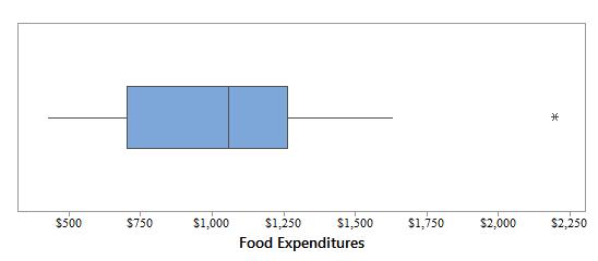
The data are skewed to the right (that is, toward smaller values).

3.79

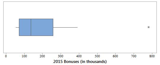
Upper

The data are skewed to the right (that is, toward larger values).

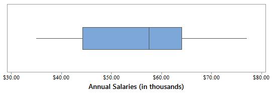
The smallest and the largest values within the two inner fences are 35 and 77, respectively. The data set contains no outliers.

The data are skewed to the left.

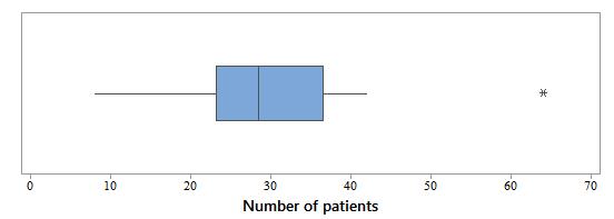
3.80 The ranked data are:

8 16 19 20 22 23 24 24 26 26

28 29 30 32 33 34 35 37 37 38

38 42 64

Median = (28 + 29)/2 = 28.5, Q 1 = 23.5, and Q 3 = 36

IQR = Q 3 – Q 1 = 12.5, 1.5 × IQR = 1.5 × 12.5 = 18.75,

Lower inner fence = Q 1 – 18.75 = 4.75

Upper inner fence = Q 3 + 18.75 = 54.75

The largest value exceeds the upper fence and so, is an outlier.

3.81

The data are skewed to the right.

a. x = (Σx)/n = 1209/22 = $54.95 thousand

Median = average of the 11th and 12th terms of the ranked data set = (45+48)/2 = $46.5 thousand

The modes are 27, 40, 43, and 86 since they each occur twice and all other values once.

b. For the 10% trimmed mean, we must remove 0.10(22) = 2.2, or 2, values from each end of the ranked data set and average the remaining 18 values to get 971/18 = $53.94 thousand

c. xx 2

Median = value of the 6.5th term in ranked data = (7 + 8)/2 = 7.5 citations Mode = 4, 7, and 8 citations

b. Range = Largest value – Smallest value = 14 – 0 = 14 citations

c. The values of the summary measures in parts a and b are sample statistics because the data are based on a sample of 12 drivers.

3.83 Weighted mean = 483($1630)1324($625)856($899)633($1178)394($1727)1138($923)

3.84 Weighted mean = 3216($425)1828($1299)4036($369)3142($681)1662($1999)

The values of these summary measures are sample statistics since they are based on a sample of 50 cities.

3.86 a. i. Each of the two values is 40 minutes from µ = 200. Hence, k = 40/20 = 2 and 1–2

1 k = 1 –2 1 (2) = 1 – 0.25 = 0.75 or 75%.

Thus, at least 75% of the students will learn the basics in 160 to 240 minutes.

ii. Each of the two values is 60 minutes from µ = 200. Hence,

0.11

0.89 or 89%. Thus, at least 89% of the students will learn the basics in 140 to 260 minutes.

3.87

b. 1

2

1 k = 0.84 gives 2

1 k = 1 – 0.84 = 0.16 or k2 = 1 0.16 , so k = 2.5.

2.5 µσ = 200 – 2.5(20) = 150 minutes and 2.5 µσ + = 200 + 2.5(20) = 250 minutes. Thus, the required interval is 150 to 250 minutes.

a. i. Each of the two values is 15 minutes from µ = 30 minutes. Hence, k = 15/6 = 2.5 and 1 –2

1 k = 1 –2 1 (2.5) = 1 – 0.16 = 0.84 or 84%. Thus, at least 84% of patients had waiting times between 15 and 45 minutes.

ii. Each of the two values is 18 minutes from µ = 30 minutes. Hence, k = 18/6 = 3 and 1 –2

1 k = 1 –2 1 3 = 1 – 0.11 = 0.89 or 89%. Thus, at least 89% of patients had waiting times between 12 and 48 minutes.

b. 1 –2

1 k = 0.75 gives 2

1 k = 1 – 0.75 = 0.25 or k2 = 1 0.25 , so k = 2. 2 µσ = 30 – 2(6) = 18 minutes and 2 µσ + = 30 + 2(6) = 42 minutes. Thus, the required interval is 18 to 42 minutes.

3.88 µ = 200 minutes and σ = 20 minutes

a. i. The interval 180 to 220 minutes is µσ to µσ + . Thus, approximately 68% of the students will learn the basics in 180 to 220 minutes.

ii. The interval 160 to 240 minutes is 2 µσ to 2 µσ + . Hence, approximately 95% of the students will learn the basics in 160 to 240 minutes.

b. 3 µσ = 200 – 3(20) = 140 minutes and 3 µσ + = 200 + 3(20) = 260 minutes. The interval that contains the learning time of 99.7% of the students is 140 to 260 minutes.

3.89 The ranked data are: 56 59 60 68 74 78 84 97 107 382

a. The three quartiles are Q 1 = 60, Q 2 = (74 + 78)/2 = 76, and Q 3 = 97

IQR = Q 3 – Q 1 = 97 – 60 = 37

The value 74 falls between Q 1 and Q 2 , which indicates that it is at least as large as 25% of the data and no larger than 50% of the data.

b. kn/100 = 70(10)/100 = 7

Thus, the 70th percentile occurs at the seventh term in the ranked data, which is 84. Therefore, P 70 = 84. This means that about 70% of the values in the data set are smaller than or equal to 84.

c. Seven values in the given data are smaller than 97. Hence, the percentile rank of 97 = (7/10) × 100 = 70%. This means approximately 70% of the values in the data set are less than 97.

3.90 The ranked data are: 27 27 28 35 36 38 40 40 43 43 45 48 50 58 62 72 77 84 86 86 90 94

a. The quartiles are:

Q 1 = 6th term in ranked data set 38

Q 2 = average of 11th and 12th term in ranked data set = (45 + 48)/2 = 46.5

Q 3 = 17th term in ranked data set = 77

IQR = Q 3 – Q 1 = 77

38 = 39

The value 77 is Q 3 which means it lies in the fourth 25% group from the bottom in the ranked data set. So, it is at least as large as 75% of the data.

b. kn/100 = 18(22)/100 = 3.96

Thus, the 18th percentile can be approximated by the value of the 4th term in the ranked data, which is 35. Therefore, P 18 = 35.

c. Fifteen values in the given data are smaller than 72. Hence, the percentile rank of 72 = (15/22) × 100 = 68%.

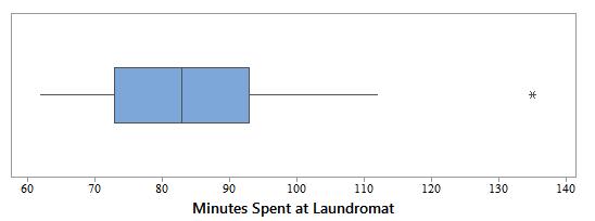
3.91 The ranked data are: 62 67 72 73 75 77 81 83 84 85 90 93 107 112 135

Median = 83, Q 1 = 73, and Q 3 = 93,

IQR = Q 3 – Q 1 = 93 – 73 = 20, 1.5 × IQR = 1.5 × 20 = 30, Lower inner fence = Q 1 – 30 = 73 – 30 = 43, Upper inner fence = Q 3 + 30 = 93 + 30 = 123

The smallest and largest values within the two inner fences are 62 and 112, respectively. The value 135 is an outlier.

The data are skewed to the right.

3.92 Let y = Melissa’s score on the final exam. Then, her grade is 756987

5 y +++ . To get a B, she needs this to be at least 80. So we solve, 756987 80 5

5(80)756987 400231 169

3.93

y y y y

+++ = =+++ =+ =

Thus, the minimum score that Melissa needs on the final exam in order to get a B grade is 169 out of 200 points.

a. Let y = amount that Jeffery suggests. Then, to insure the outcome Jeffery wants, we need 12,000(5) 20,000

y y y y

+ = += += =

6 12,000(5)6(20,000) 60,000120,000 60,000

So, Jeffery would have to suggest $60,000 be awarded to the plaintiff.

b. To prevent a juror like Jeffery from having an undue influence on the amount of damage to be awarded to the plaintiff, the jury could revise its procedure by throwing out any amounts that are outliers and then recalculate the mean, or by using the median, or by using a trimmed mean.

3.94

a. To calculate how much time the trip requires, divide miles driven by miles per hour for each 100 mile segment. Then, time = 100/52 + 100/65 + 100/58 = 1.92 + 1.54 + 1.72 = 5.18 hours.

b. Linda’s average speed for the 300 mile trip is not equal to (52 + 65 + 58)/3 = 58.33 mph. This would assume that she spent an equal amount of time on each 100 mile segment, which is not true, because her average speed is different on each segment. Linda’s average speed for the entire 300 mile trip is given by (miles driven)/(elapsed time) = 300/5.18 = 57.92 mph.

3.95 a. Total amount spent per month by the 2000 shoppers = (14)(8)(1100) + (18)(11)(900) = $301,400

b. Total number of trips per month by the 2000 shoppers = (8)(1100) + (11)(900) = 18,700

Mean number of trips per month per shopper = 18,700/2000 = 9.35 trips

c. Mean amount spent per person per month by shoppers aged 12−17 = 301,400/2000 = $150.70

3.96

a. For people age 30 and under, we have the following death rates from heart attack:

So the death rate for people 30 and under is lower in Country B.

b. For people age 31 and older, the death rates from heart attack are as follows:

Thus, the death rate for Country A is greater than that for Country B for people age 31 and older.

c. The overall death rates are as follows:

Thus, overall the death rate for country A is lower than the death rate for Country B.

d. In both countries people age 30 and under have a lower percentage of death due to heart attack than people age 31 and over. Country A has 2/3 of its population age 30 and under while more than 1/2 of the people in Country B are age 31 and over. Thus, more people in Country B than in County A fall into the higher risk group which drives up Country B’s overall death rate from heart attacks.

3.97 µ = 70 and σ = 10

a. Using Chebyshev’s theorem, we need to find k so that at least 1 – 0.50 = 0.5 of the scores are within k standard deviations of the mean.

3.98

3.99

1 –2

1 k = 0.50 gives 2

1 k = 1 – 0.50 = 0.50 or k2 = 1 0.50 = 2, so k= 2 ≈ 1.41. Thus, at least 50% of the scores are within 1.41 standard deviations of the mean.

b. Using Chebyshev’s theorem, we first find k so that at least 1 –0.20 =0 .80 of the scores are within k standard deviations of the mean.

1 –2

1 k = 0.80 gives 2

1 k = 1 – 0.80 = 0.20 or k2 = 1 0.20 = 5, so k= 52.24 »

Thus, at least 80% of the scores are within 2.24 standard deviations of the mean, but this means that at most 10% of the scores are greater than 2.24 standard deviations above the mean.

a. Since we are dealing with a bell-shaped distribution and we know that 16% of all students scored above 85, which is µ + 15, we must also have that 16% of all students scored below µ – 15 = 55. Therefore, the remaining 68% of students scored between 55 and 85. By the empirical rule, we know that approximately 68% of the scores fall in the interval µσ to µσ + , so we have µσ = 70 σ = 55 and µσ + = 70 σ + = 85. Thus, 15. σ =

b. We know that 95% of the scores are between 60 and 80 and that µ = 70. By the empirical rule, 95% of the scores fall in the interval 2 µσ to 2 µσ + . Then 60 = 2 µσ = 702σ and 80 = 2 µσ + = 702σ + . Therefore, 1025. σσ =⇒=

a. Mean = $600.35, Median = $90, and Mode = $0

b. The mean is the largest.

c. Q 1 = $0, Q 3 = $272.50, IQR = $272.50, 1.5 × IQR = $408.75

Lower inner fence is Q 1 – 408.75 = 0 – 408.75 = –408.75

Upper inner Fence is Q 3 + 408.75 = 272.50 +408.75 = 681.25

The largest and smallest values within the two inner fences are 0 and 501, respectively. There are three outliers at 1127, 3709 and 14,589.

Below is the box–and–whisker plot for the given data.

The data are strongly skewed to the right.

d. Because the data are skewed to the right, the insurance company should use the mean when considering the center of the data as it is more affected by the extreme values. The insurance company would want to use a measure that takes into consideration the possibility of extremely large losses.

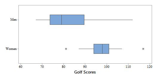
3.100 a.

The box–and–whisker plots show that the men’s scores tend to be lower and more varied than the women’s scores. The men’s scores are skewed to the right, while the women’s are more nearly symmetric.

b. Men Women

x = 82

Median = 79

x = 97.53

Median = 98

Modes = 75, 79, and 92 Modes = 94 and 100

Range = 45 Range = 36

s 2 = 145.8750

s = 12.08

Q 1 = 73.5

Q 3 = 89.5

IQR = 16

s 2 = 71.2667

s = 8.44

Q 1 = 94

Q 3 = 101

IQR = 7

These numerical measures confirm the observations based on the box–and–whisker plots.

3.101 a. Since x = (Σx)/n, we have n = (Σx)/ x = 12,372/51.55 = 240 pieces of luggage.

b. Since x = (Σx)/n, we have (Σx) = nx = (7)(81) = 567 points. Let x = seventh student’s score. Then, x + 81 + 75 + 93 + 88 + 82 + 85 = 567. Hence, x + 504 = 567, so x = 567 – 504 = 63.

3.102 For all students: n = 44, Σx = 6597, Σx 2 = 1,030,639, and median = 147.50 pounds x = (Σx)/n = 6597/44 = 149.93 pounds

For men only: n = 22, Σx = 3848, Σx 2 = 680,724 and median = 179 pounds x = (Σx)/n = 3848/22 = 174.91 pounds

= 22, Σx = 2749, Σx 2 = 349,915 and median = 123 pounds x = (Σx)/n = 2749/22 = 124.95 pounds

In this case, the median may be more informative than the mean, since it is less influenced by extremely high or low weights. As one might expect, the mean and median weights for men are higher than those of women. For the entire group, the mean and median weights are about midway between the corresponding values for men and women. The standard deviations are roughly the same for men and women. The standard deviation for the whole group is much larger than for men or women only, due to the fact that it includes the lower weights of women and the heavier weights of men.

3.103 The ranked data are: 3 6 9 10 11 12 15 15 18 21 25 26 38 41 62

a. x = 20.80 thousand miles, Median = 15 thousand miles, and Mode = 15 thousand miles

b. Range = 59 thousand miles, s 2 = 249.03, s = 15.78 thousand miles

c. Q 1 = 10 thousand miles and Q 3 = 26 thousand miles

d. IQR = Q 3 – Q 1 = 26 – 10 = 16 thousand miles

Since the interquartile range is based on the middle 50% of the observations it is not affected by outliers. The standard deviation, however, is strongly affected by outliers. Thus, the interquartile range is preferable in applications in which a measure of variation is required that is unaffected by extreme values.

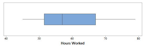
3.104 x = 49.012 hours and s = 5.080 hours

a. For 75%: 1 –2 1 k = 0.75 gives

0.8889 = .1111 or k2 = 1 0.1111 , so k ≈ 3. 3 xs = 49.012 – 3(5.080) = 33.77 and 3 xs + = 49.012 + 3(5.080) = 64.25 Thus, the required interval is 33.77 to 64.25 hours.

For 93.75%: 1 –2

1 k = 0.9375 gives

0.9375 = 0.0625 or k2 = 1 0.0625 , so k = 4. = 49.012 – 4(5.080) = 28.69 and 4 xs + = 49.012 + 4(5.080) = 69.33 Thus, 4 xs the required interval is 28.69 to 69.33 hours.

1 k = 1

2

b. 100% of the data falls into each of the intervals calculated in part a.

xs = 49.012 – (5.080) = 43.93 and xs + = 49.012 + (5.080) = 54.09 Twenty-eight or 56% of the observations fall within one standard deviation of the mean.

c. The endpoints provided by Chebyshev's Theorem are not useful since each of these intervals contain all of the data points.

d. With the change in the sample mean and standard deviations, the required intervals are 35.41 to 63.81 hours for 75%, 28.31 to 70.91 hours for 88.89%, and 21.21 to 78.01 hours for 93.75%. Each of these intervals contains 98% of the data which is a small change from 100%. The only value not included in

these intervals is the outlier at 84.4 hours. Now, 39 or 78% of the observations fall within one standard deviation of the mean (between 42.51 and 56.71). This is a relatively large increase from the 56% found in part b.

e. Using the upper endpoint of 58.7, we have 58.7 = 49.012 + k(5.08). Then k = 1.907. We would have to go 1.907 standard deviations about the mean to capture all 50 data values. By Chebyshev's Theorem, the lower bound for the percentage of data that would fall in this interval is

2 2

11 11 1.2750 (1.907) 0 k −=−=− ,0.7250 = or 72.50%.

Self–Review Test

1. b 2. a and d 3. c

4. c 5. b 6. b

7. a 8. a 9. b

10. a 11. b 12. c

13. a 14. a

15.

a. x = (Σx)/n = 420/20 = 21 times Median = average of the 10th and 11th terms of the ranked data set = (13 + 14)/2 = 13.5 times The modes are 5, 8, and 14 since they each occur twice and all other values once.

b. For the 10% trimmed mean, we must remove 0.10(2) = 2 values from each end of the ranked data set and average the remaining 16 values to get 251/16 = 15.6875 times

d. Coefficient of variation = 23.1 100%100%110.1%

e. These are sample statistics because a subset of all people using debit cards was used, not ALL such people.

16. Weighted mean = ( 2842($2055) + 4364($1165) + 3946($1459) + 1629($2734) + 3871($1672) ) / 16,652 = $1,657.914

17. Suppose the exam scores for seven students are 73, 82, 95, 79, 22, 86, and 91 points. Then, mean = (73 + 82 + 95 + 79 + 22 + 86 + 91)/7 = 75.43 points. If we drop the outlier (22), then mean = (73 + 82 + 95 + 79 + 86 + 91)/6 = 84.33 points. This shows how an outlier can affect the value of the mean.

18. Suppose the exam scores for seven students are 73, 82, 95, 79, 22, 86, and 91 points. Then, range = largest value – smallest value = 95 – 22 = 73 points. If we drop the outlier (22) and calculate the range, range = largest value – smallest value = 95 – 73 = 22 points. Thus, when we drop the outlier, the range decreases from 73 to 22 points.

19. The value of the standard deviation is zero when all the values in a data set are the same. For example, suppose the heights (in inches) of five women are: 67 67 67 67 67 This data set has no variation. As shown below the value of the standard deviation is zero for this data set. For these data: n = 5, Σx = 335, and Σx 2 = 22,445.

20.

a. The frequency column gives the number of weeks for which the number of computers sold was in the corresponding class.

b. For the given data: n = 25, Σmf = 486.50, and Σm 2f = 10,524.25 x = (Σmf)/n = 486.50/25 = 19.46 computers

21.

a. i. Each of the two values is 32.4 minutes from µ = 91.8 minutes. Hence, k = 32.4/16.2 = 2 and 2 2

11 111.25. 0 5 2 0 7 k −=−=−= or 75%. Thus, 75% of the members spent between 59.4 and 124.2 minutes at the health club.

ii. Each of the two values is 40.5 minutes from µ = 91.8 minutes. Hence, k = 40.5/16.2 = 2.5 and 2 2

11 111.16.84 2.5 00 k −=−=−= or 84%. Thus, 84% of the members spent between 51.3 and 132.3 minutes at the health club.

b. 22 2 22

1111 1.891.89.11 93 .1 000 0 1 kkk kkk −=⇒−=⇒=⇒=⇒≈⇒= ( ) 391.8316.243.2µσ−=−= minutes and ( ) 91.8316.2140.4 3 µσ =+= + Thus, the required interval is 43.2 minutes to 140.4 minutes.

22. µ = 7.3 years and σ = 2.2 years

a. i. The interval 5.1 to 9.5 years is µσ to µσ + . Hence, approximately 68% of the cars are 5.1 to 9.5 years old.

ii. The interval 0.7 to 13.9 years is 3 µσ to 3 µσ + . Hence, approximately 99.7% of the cars are 0.7 to 13.9 years.

b. 2 µσ = 7.3 – 2(2.2) = 2.9 hours and 2 µσ + = 7.3 + 2(2.2) = 11.7 hours. The interval that contains ages of 95% of the cars will be 2.9 to 11.7 years.

23. The ranked data are:

a. Median = (56 + 58)/2 = 57, Q 1 = 52, and Q 3 = 66

66 – 52 = 14,

The value 54 lies between Q 1 and the Median, so it is in the second 25% group from the bottom of the ranked data set. This means that 25% of the data is less than 54 and that at least 50% of the data is larger than 54.

b. kn/100 = 60(18)/100 = 10.8

Thus, the 60th percentile can be approximated by the 11th term in the ranked data. Therefore, P 60 = 61. This means that 60% of the values in the data set are less than 61.

c. Twelve values in the given data set are less than 64. Hence, the percentile rank of 64 = (12/18) × 100 = 66.7% or about 67%.

24.

The data is skewed to the right.