ON DECREASING OF DIMENSIONS OF FIELDEFFECT TRANSISTORS WITH SEVERAL SOURCES by journalmsej

Advances in Materials Science and Engineering: An International Journal (MSEJ), Vol. 3, No. 3, September 2016

ON DECREASING OF DIMENSIONS OF FIELDEFFECT TRANSISTORS WITH SEVERAL SOURCES E.L. Pankratov, E.A. Bulaeva Nizhny Novgorod State University, 2 Gagarin avenue, Nizhny Novgorod, 603950, Russia

ABSTRACT We analyzed mass and heat transport during manufacturing field-effect heterotransistors with several sources to decrease their dimensions. Framework the result of manufacturing it is necessary to manufacture heterostructure with specific configuration. After that it is necessary to dope required areas of the heterostructure by diffusion or ion implantation to manufacture the required type of conductivity (p or n). After the doping it is necessary to do optimize annealing. We introduce an analytical approach to prognosis mass and heat transport during technological processes. Using the approach leads to take into account nonlinearity of mass and heat transport and variation in space and time (at one time) physical parameters of these processes

KEYWORDS Field-effect transistor, transistor with several channels, increasing of compactness of transistors

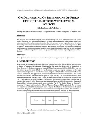
1. INTRODUCTION Now several problems of solid state electronic intensively solving. The problems are increasing of density of elements of integrated circuits and at the same time decreasing of dimensions of these elements [1-4], increasing performance [5-7] and increasing reliability [8,9]. Now one can find intensive development of both power electronic devices and logical elements. In this paper we consider an approach to manufacture more compact field-effect heterotransistor with several sources. Framework the approach it is necessary to manufacture a heterostructure. The heterostructure consist of a substrate and an epitaxial layer (see Fig. 1). Several sections have been manufactured into the epitaxial layer. These sections manufactured by using other materials (see Fig. 1). The sections have been doped by diffusion or ion implantation to obtain required type of conductivity (n or p). After the doping one can manufacture a field-effect transistor framework the considered heterostructure so as it is shown on the Fig. 1. The doping should be finished by annealing of dopant and/or radiation defects. The annealing should be optimized. The optimization attracted an interest to manufacture more compact distributions of concentrations of dopant. Framework the paper we formulate conditions to increase compactness and at the same time to increase homogeneity of distribution of concentration of dopant in enriched by the dopant area.

Fig. 1. Structure of a field-effect heterotransistor. Top side of the structure DOI:10.5121/msej.2016.3301

Advances in Materials Science and Engineering: An International Journal (MSEJ), Vol. 3, No. 3, September 2016

2. METHOD OF SOLUTION To solve our aim we determine distribution of concentration of dopant C(x,y,z,t) in space and time. To determine the distribution we solve the following boundary problem ∂ C ( x, y , z , t ) ∂  ∂ C ( x, y , z , t )  ∂ = D + ∂t ∂x ∂x  ∂y

 ∂ C ( x, y , z , t )  ∂ D + ∂y   ∂z

∂ C ( x, y , z , t ) ∂ C ( x, y , z , t ) ∂ C ( x, y , z , t ) =0, = 0, ∂x ∂x ∂y x =0 x = Lx

 ∂ C ( x, y , z , t )  D  ∂z  

= 0, y =0

(1)

∂ C ( x, y , z , t ) =0, ∂y x=Ly

∂ C ( x, y , z , t ) ∂ C ( x, y , z , t ) =0, = 0 , C x,y,z,0)=fC (x,y,z). ∂z ∂z z =0 x = Lz (

(2)

Here T is the temperature of annealing; DС is the dopant diffusion coefficient. Dopant diffusion coefficient takes another value in other materials. Heating and cooling of heterostructure (see Arrhenius law) also leads to changing of value of diffusion coefficient. We consider following approximation of concentrational dependences of dopant diffusion coefficient [10-12]  C γ ( x, y , z , t )   V ( x, y , z , t ) V 2 ( x, y , z , t )  DC = DL ( x, y, z, T ) 1 + ξ γ +ς2 1 + ς 1 .  * P (x, y , z, T )   V (V * )2  

(3)

Here function DL (x,y,z,T) describes dependences of dopant diffusion coefficient on coordinate and temperature; function P (x,y,z,T) describes dependences of limit of solubility on coordinate and temperature; parameter γ ∈[1,3] is integer and depends on properties of materials; function V (x,y,z,t) describes distribution of concentration of radiation vacancies on space and time with equilibrium distribution V*. Dependence of dopant diffusion coefficient on concentration of dopant has been investigated and described in details in [10]. Diffusion of dopant gives a possibility to dope materials without generation radiation defects. In this situation ζ1= ζ2= 0. Ion doping of dopant leads to generation radiation defects. Distributions of concentrations of point radiation defects have been determined by solving the following boundary problem [11,12]

∂ I (x, y, z, t ) ∂  ∂ I ( x, y, z, t )  ∂  ∂ I (x, y, z, t )  =  DI (x, y, z, T ) +  DI ( x, y, z, T )  − k I , I (x, y, z, T ) × ∂t ∂x ∂x ∂y  ∂y  × I 2 ( x, y , z , t ) +

∂ I ( x, y , z , t )  ∂   D I ( x, y , z , T )  − k I ,V ( x, y, z, T ) I ( x, y, z , t ) V ( x, y , z, t ) (4) ∂z  ∂z 

∂ V (x, y, z, t ) ∂  ∂ V (x, y, z, t )  ∂  ∂ V ( x, y, z, t )  = DV (x, y, z, T ) + DV ( x, y, z, T )  − kV ,V (x, y, z, T ) × ∂t ∂x ∂x ∂y  ∂y  × V 2 ( x, y , z , t ) +

∂ V ( x, y , z , t )  ∂   DV (x, y , z , T )  − k I ,V ( x, y , z, T ) I ( x, y , z, t ) V (x, y , z , t ) ∂z  ∂z 

∂ ρ (x, y, z, t ) ∂ ρ (x, y , z , t ) ∂ ρ ( x, y , z , t ) ∂ ρ ( x, y , z , t ) =0, =0, =0, = 0, ∂ y ∂y ∂x ∂ x y =0 y= Ly x=0 x = Lx ∂ ρ ( x, y , z , t ) ∂ ρ ( x, y , z , t ) =0, = 0 , ρ (x,y,z,0)=fρ (x,y,z). ∂z ∂z z =0 z=L

(5)

Advances in Materials Science and Engineering: An International Journal (MSEJ), Vol. 3, No. 3, September 2016

Here ρ =I,V; distribution of concentration of radiation interstitials in space and time describes by the function I (x,y,z,t); terms of Eqs.(4) with quadric concentrations of point radiation defects (V2(x,y,z,t) and I2(x,y,z,t)) correspond to generation of simplest complexes of radiation defects (divacancies and diinterstitials); temperature and spatial dependences of diffusion coefficients of point radiation defects describe by functions Dρ(x,y,z,T); temperature and spatial dependences of parameter of recombination of point radiation defects describe by function kI,V(x,y,z,T); functions kI,I(x,y,z,T) and kV,V(x,y,z,T) describe spatial and temperature dependences of parameters of generation of simplest complexes of point radiation defects. Concentrations of divacancies ΦV (x,y,z,t) and dinterstitials ΦI (x,y,z,t) have been calculated by solution of the following boundary problem [11,12]

∂ Φ I ( x, y, z, t ) ∂  ∂ Φ I ( x, y, z, t )  ∂  ∂ Φ I ( x, y, z, t )  = D ( x, y, z, T )  + ∂ y  DΦI ( x, y, z, T ) + ∂t ∂ x  ΦI ∂x ∂y    +

∂  ∂ Φ I ( x, y, z, t )  DΦI (x, y, z, T ) + kI ,I (x, y, z, T ) I 2 (x, y, z, t ) − kI ( x, y, z, T ) I ( x, y, z, t )   ∂z ∂z 

(6)

∂ ΦV (x, y, z, t ) ∂  ∂ ΦV (x, y, z, t )  ∂  ∂ ΦV (x, y, z, t ) = DΦV (x, y, z,T ) + DΦV (x, y, z, T )    + ∂t ∂x ∂x ∂y  ∂y  +

∂  ∂ ΦV (x, y, z, t )  2 DΦV (x, y, z, T )   + kV ,V (x, y, z, T ) V (x, y, z, t ) − kV ( x, y, z, T ) V (x, y, z, t ) ∂z ∂z 

∂ Φ ρ ( x, y , z , t ) ∂x

=0, x =0

∂ Φ ρ ( x, y , z , t ) ∂z

=0, z =0

∂ Φ ρ ( x, y , z , t ) ∂x

=0, x = Lx

∂ Φ ρ ( x, y , z , t ) ∂z

∂ Φ ρ ( x, y , z , t ) ∂y

= 0, y =0

∂ Φρ (x, y, z, t ) ∂y

=0, y=Ly

= 0 , ΦI (x,y,z,0)=fΦI (x,y,z), ΦV (x,y,z,0)=fΦV (x,y,z). (7) z = Lz

Functions DΦρ(x,y,z,T) describe spatial and temperature dependences of diffusion coefficients of simplest complexes of point radiation defects; functions kI(x,y,z,T) and kV (x,y,z,T) describe spatial and temperature dependences of parameters of decay of the above complexes. Now let us consider equivalent integro-differential form of Eq.(1) t y z  xyz x y z V (x, v, w,τ ) V 2 (x, v, w,τ )  + ς × ∫ ∫ ∫ C (u, v, w, t ) d w d v d u = ∫ ∫ ∫ DL (x, v, w, T ) 1 + ς 1 2 L x L y L z Lx L y Lz V* 0 L y Lz (V * )2  

 yz xz t x z ∂ C (u, y, w,τ ) C γ (x, v, w,τ )  ∂ C (x, v, w, τ ) × 1 + ξ γ dτ + × ∫ ∫ ∫ DL (u, y, w, T )  L y L z L x L z 0 Lx Lz ∂ y ∂ x P (x, v, w, T )    V (u , y , w,τ ) xy t x y V 2 (u , y , w,τ )   C γ (u , y , w,τ )  × 1 + ς 1 + ς 1 + ξ  ∫ ∫ ∫ D L (u , v, z , T ) × 2   dτ + * 2 γ * V L x L y 0 Lx L y (V )   P (x, y, z, T )    V (u , v, z ,τ ) V 2 (u , v, z ,τ )   C γ (u , v, z ,τ )  ∂ C (u , v, z ,τ ) xyz × 1 + ς 1 + 1 + dτ + × ς ξ  2   γ * * 2 V Lx L y Lz (V )   P (x, y, z, T ) ∂ z  x y z

× ∫ ∫ ∫ f (u , v, w) d w d v d u .

(1a)

Lx L y Lz

Advances in Materials Science and Engineering: An International Journal (MSEJ), Vol. 3, No. 3, September 2016

We used the Bubnov-Galerkin approach [13] to calculate solution of the above equation. To use the approach we consider of the Eq.(1a) as the following series N

C0 ( x, y , z, t ) = ∑ a nC cn (x ) cn ( y ) cn (z ) enC (t ) . n=0

[

]

Here enC (t ) = exp − π 2 n 2 D0C t (L−x2 + L−y2 + L−z2 ) , cn(χ) = cos (π n χ/Lχ). Number of terms N of the above series is finite. The series is almost coincides with solution of Eq.(1) in the linear case (i.e. with ξ = 0) and average value of dopant diffusion coefficient D0. Framework the approach we substitute the above series into Eq.(1a). After the substitution we obtain γ t y z N aC  ξ ∑  s ( x ) s ( y ) s ( z ) e ( t ) 1 a c ( x ) c ( v ) c ( w ) e ( ) = − + τ ∫ ∫ ∫  × n n n nC nC n n n nC 3 γ   n =1 n n =1  P (x, v, w, T ) 0 L y Lz 

xyz

∑

π2

 N V (x, v, w,τ ) yz V 2 (x, v, w,τ )  DL (x, v, w, T ) ∑ n a nC s n (x ) c n (v ) c n (w) e nC (τ ) d τ × 1 + ς 1 + ς −  2 * 2 * n = 1 V L (V )  y Lz  −

γ xz t x z V (u, y, w, τ ) V 2 (u, y, w, τ )    N  × ( ) ( ) ( ) ( ) 1 + ς + ς 1 + a c u c y c w e τ ∑   ∫∫∫  1 2 L x L z 0 Lx Lz  V* (V * )2   m=1 mC m m m mC 

N  xy t x y ∫ ∫ ∫ D L (u , v, z, T ) ×  D L (u , y , w, T ) ∑ n a nC c n (u ) s n ( y ) c n (w ) e nC (τ ) d τ − n =1 L x L y 0 Lx L y P (u , y , w, T ) 

γ N   ξ V (u , v, z ,τ ) V 2 (u , v, z ,τ )  ∑ × 1 + γ anC cn (u ) cn (v ) cn (z ) enC (τ )  1 + ς 1 + × ς 2    V* (V * )2   P (u , v, z , T )  n =1  N

× ∑ n a nC c n (u ) c n (v ) s n ( z ) e nC (τ ) d τ + n =1

xyz x y z ∫ ∫ ∫ f (u , v, w) d w d v d u . L x L y L z Lx L y Lz

(8)

Here sn(χ) = sin (π n χ/Lχ). To determine coefficients an it is necessary to use orthogonality condition of terms of the above series framework scale of heterostructure. Using the condition leads to the following equations to calculate of coefficients an for any quantity of terms N −

L2x L2y L2z

π5

γ t L x L y Lz a nC  N  ξ  ( ) ( ) ( ) ( ) ( ) ( ) τ e t D x , y , z , T 1 a c x c y c z e = − + ∑ ∫ ∫ ∫ ∫  × nC L nC n n n nC 6 γ   n =1 n  P ( x, y, z, T )  0 0 0 0  n =1 N

∑

L y Lz  Ly   V ( x, y , z , τ ) V 2 ( x, y , z, τ )  N a nC [c n ( y ) − 1] × 1 + ς1 +ς2 s n (2 x ) c n ( y )  y s n ( y ) + ∑  2  * 2 * n = 1 2 π  V n π n (V )   

γ t Lx L y Lz  N   L × cn (z ) enC (τ )  z sn (z ) + z [cn (z ) − 1] d z d y d x d τ − ∫ ∫ ∫ ∫  ∑ anC cn ( x ) cn ( y ) cn ( z ) enC (τ ) ×  n =1 πn 0 0 0 0   

  V ( x, y , z , τ ) V ( x, y , z , τ ) V 2 ( x, y , z , τ )   + 1 D L (x, y , z , T ) 1 + ς 1 +ς2 +  1 + ς 1 * * 2 P ( x, y , z , T )  V V* (V )   

+ς2

  L V 2 ( x, y , z,τ )  N anC Lz  L x sn (x ) + x [cn ( x ) − 1] z sn ( z ) + z [cn ( z ) − 1]cn ( x ) sn (2 y ) cn ( z ) × ∑ 2  * 2 πn πn (V )  n=1 2π n   

× enC (τ ) d z d y d x d τ −

γ t Lx L y Lz   ξ N  ∫ ∫ ∫ ∫ 1 +  ∑ anC cn ( x ) cn ( y ) cn ( z ) enC (τ ) γ ×  P ( x, y , z , T )  2 π 0 0 0 0  n=1

Lx L y 2

Advances in Materials Science and Engineering: An International Journal (MSEJ), Vol. 3, No. 3, September 2016

   L V (x, y , z,τ )  N a nC V 2 ( x, y , z , τ ) × D L (x, y , z, T ) 1 + ς 2 + ς1 c n ( x )  x s n ( x ) + x [c n ( x ) − 1] × ∑ * * 2 V πn (V )   n =1 n  

Ly N Lx   [c n ( y ) − 1] enC (τ ) d z d y d x d τ + ∑ ∫  x s n (x ) + L x [c n (x ) − 1] × × c n ( y ) s n (z )  y s n ( y ) + n =1 0 πn πn     Ly Lz Ly  [cn ( y ) − 1] ∫  z sn (z ) + Lz [cn (z ) − 1] f (x, y, z ) d z d y d x . × ∫  y sn ( y ) + πn πn 0  0

(9)

Now we consider several examples. For γ = 0 we obtain Lx L y  Lz Ly L [cn ( y ) − 1] ∫  z sn (z ) + y [cn (z ) − 1] f (x, y, z ) d z d y  x sn (x ) + Lx × anC = ∫ ∫  y sn ( y ) + πn πn πn 0 0   0 

Ly Lz  n  t Lx Ly  [cn (z ) − 1]{ y sn ( y ) + × [cn ( x ) − 1]}d x  ∫ ∫ sn (2 x ) ∫ cn ( y ) ∫ cn (z ) DL (x, y , z , T ) z sn (z ) +  2 0 0 π n 0 0    

πn

 [c ( y ) − 1] 1 + ς V (x, y, z ,τ ) + ς n

 

 V 2 ( x, y , z ,τ )   ξ  1 + γ  cn ( z ) d z d y d x × * 2 P ( x , y , z , T ) (V )   

Ly Lx Lz t Ly L  × enC (τ ) d τ + ∫ enC (τ ) ∫ cn ( x )  x sn (x ) + [cn (x ) − 1] ∫ sn (2 y ) ∫ cn (z )  z sn (z ) + y [cn (z ) − 1] × πn πn 0 0 0    0

  ξ V ( x , y , z ,τ ) V 2 ( x, y , z ,τ )  × DL (x, y , z , T ) 1 + γ 1 + ς + ς d z d y d xdτ +  1 2  V* (V * )2   P ( x, y, z , T )   Lx Lz t Ly  Ly  L + ∫ enC (τ ) ∫ cn ( x )  x sn (x ) + x [cn (x ) − 1] ∫ cn ( y )  y sn ( y ) + [cn ( y ) − 1]  ∫ DL (x, y, z, T ) × πn πn 0 0  0  0

  V (x, y, z,τ )  V 2 (x, y, z,τ ) ξ ς × s n (2 z ) 1 + γ 1 + + ς1   d z d y d x dτ 2  2 * V* (V )  P (x, y, z, T )   

 L2 L2 L2 z z z − 5 6 π n 

−1

  .(10)  

For γ = 1 calculation of parameters an leads to the following results a nC = −

Here α n =

Ly Lx Lz βn ± β n2 + 4α n ∫ c n ( x ) ∫ c n ( y ) ∫ cn (z ) f ( x, y, z ) d z d y d x . 2α n 0 0 0

(11)

Ly Lz ξ L y L z t Lx D L ( x, y , z , T )  V ( x, y , z , τ ) V 2 ( x, y , z , τ )  ( ) ( ) ς ς s 2 x c y 1 + +   × ∫∫ n ∫ n ∫ 1 2 2π 2n 0 0 V* 0 0 P ( x, y , z , T )  (V * )2  

Ly   × c n (z )  y s n ( y ) + [c n ( y ) − 1] z s n (z ) + L z [c n (z ) − 1] d z d y d x enC (τ ) d τ + ξ L x2Lz × πn πn 2π n    L Lx Lz t  y L D (x, y , z , T )  Lz × ∫ e nC (τ ) ∫ c n (x )  x s n (x ) + x [c n ( x ) − 1] ∫ s n (2 y ) ∫ L [c n (z ) − 1] ×  z s n (z ) − πn πn 0 0 0 P ( x, y , z , T )   0  2 Ly Lx t   L L ξ V (x, y , z ,τ ) V (x, y , z ,τ ) x y × cn (z ) 1 + ς 1 +ς2  d z d yd xdτ + ∫ enC (τ ) ∫ cn ( x ) ∫ cn ( y ) × * 2 * 2 π V 2 n 0 0 0 (V )   5

Advances in Materials Science and Engineering: An International Journal (MSEJ), Vol. 3, No. 3, September 2016 Lz

× ∫ s n (2 z ) 0

×y +

πn

Lx D L ( x, y , z , T )  V ( x, y , z , τ ) V 2 ( x, y , z , τ )   [c n (x ) − 1]{ s n ( y ) × ς + 1 + ς 1   x s n (x ) + 2 * 2 * πn P (x, y , z , T )  V (V )   



[c ( y ) − 1]  d z d y d x d τ , n



βn =

L y Lz 2 nπ

∫ enC (τ ) ∫ s n (2 x ) ∫ c n ( y ) ∫ c n ( z ) DL (x, y, z, T ) ×

 L Lz V (x, y , z ,τ ) V 2 ( x , y , z ,τ )   ς × 1 + ς 1 + [cn (z ) − 1] d z  y [cn ( y ) − 1] + y sn ( y ) ×   z sn (z ) + 2 * * 2 V πn (V )     π n  Ly Lx L t z   LL L V (x, y, z,τ )  × d y d x d τ + x z2 ∫ enC (τ ) ∫ cn (x )  x s n (x ) + x [cn (x ) − 1] ∫ s n (2 y ) ∫ c n (z ) 1 + ς 1 + π 2 nπ 0 n V* 0 0 0    +ς2

L L t  Lz V 2 ( x, y , z , τ )  [c n (z ) − 1] d z d y d x d τ + x y2 ∫ enC (τ ) ×  D L ( x, y , z , T )  z s n ( z ) + * 2 2 nπ 0 πn (V )   

2 Lx  Ly  Lz   L y  L [cn ( y ) − 1] ∫ 1 + ς 1 V (x, y*, z,τ ) + ς 2 V (x, *y,2z,τ ) × × ∫  x s n ( x ) + x [cn ( x ) − 1] ∫  y s n ( y ) + πn πn V 0 (V )  0  0 

× sn (2 z ) DL (x, y, z, T ) d z cn ( y ) d y cn ( x ) d x d τ − L2x L2y L2z enC (t ) π 5 n 6 . It could be used the same approach to calculate values of parameters an for larger values of the parameterγ. However the relations became more bulky and will not be present in the paper. The considered approach gives a possibility to calculate distributions of concentrations of dopant and radiation defects without joining of the above concentration on interfaces of the considered heterostructure. We solved equations of the system (4) by using Bubnov-Galerkin approach. To use the approach we previously transform the differential equations to the following integro-differential form xyz x y z yz t y z ∂ I ( x, v, w,τ ) xz d wd vdτ + × ∫ ∫ ∫ I (u , v, w, t ) d w d v d u = ∫ ∫ ∫ DI ( x, v, w, T ) L x L y L z Lx L y Lz L y L z 0 L y Lz ∂x Lx Lz t x z

× ∫ ∫ ∫ DI (u , y, w, T ) 0 L x Lz

−

∂ I (u , y , w,τ ) xy t x y ∂ I (u , v, z ,τ ) d wd u dτ + d vd udτ − ∫ ∫ ∫ DI (u , v, z , T ) ∂x Lx L y 0 L x L y ∂z

xyz x y z xyz x y z ∫ ∫ ∫ k I ,V (u , v, w, T ) I (u , v, w, t ) V (u , v, w, t ) d w d v d u − ∫ ∫ ∫ k I , I (u , v, w, T ) × L x L y L z Lx L y L z L x L y L z Lx L y L z × I 2 (u , v, w, t ) d w d v d u +

xyz x y z ∫ ∫ ∫ f I (u , v, w ) d w d v d u L x L y L z L x L y Lz

(4a)

xyz x y z yz t y z ∂ V ( x, v, w,τ ) xz d wd v dτ + × ∫ ∫ ∫ V (u , v, w, t ) d w d v d u = ∫ ∫ ∫ DV ( x, v, w, T ) L x L y L z Lx L y Lz L y L z 0 L y Lz ∂x Lx Lz t x z

× ∫ ∫ ∫ DV (u, y, w, T ) 0 Lx Lz

−

∂ V (u , y, w,τ ) xy t x y ∂ V (u, v, z ,τ ) d wd u dτ + d vd u dτ − ∫ ∫ ∫ DV (u, v, z , T ) ∂x L x L y 0 Lx L y ∂z

xyz x y z xyz x y z ∫ ∫ ∫ k I ,V (u , v, w, T ) I (u , v, w, t ) V (u , v, w, t ) d w d v d u − ∫ ∫ ∫ kV ,V (u , v, w, T ) × L x L y L z Lx L y L z L x L y L z Lx L y Lz × V 2 (u , v, w, t ) d w d v d u +

xyz x y z ∫ ∫ ∫ fV (u , v, w ) d w d v d u . Lx Ly Lz Lx Ly Lz

Now we consider solutions of the above integro-differential equations as the following series 6

Advances in Materials Science and Engineering: An International Journal (MSEJ), Vol. 3, No. 3, September 2016 N

ρ 0 (x, y, z, t ) = ∑ anρ cn (x ) cn ( y ) cn (z ) enρ (t ) . n =1

Here anρ are coefficients, which should be determined. After substitution of the series into Eqs. (4a) one can obtain xyz

π3

y t z a nI y zπ N ( ) ( ) ( ) ( ) ( ) ( ) s x s y s z e t = − a e τ c y c n (z ) D I (x, v, w, T ) d w d v d τ × ∑ ∫ ∫ ∫ n n n nI nI nI n 3 n =1 n L x L y L z n =1 0 Ly Lz N

∑

× sn (x ) −

t x z x zπ N x yπ N ∑ anI sn ( y ) ∫ enI (τ ) ∫ cn (x ) ∫ cn (z ) DI (u , y, w, T ) d w d u d τ − ∑ anI sn ( z ) × Lx L y Lz n =1 Lx Ly Lz n =1 0 Lx Lz

× ∫ enI (τ ) ∫ cn (x ) ∫ cn ( y ) DI (u , v, z , T ) d v d u d τ −

× k I , I (u , v, v, T ) d w d v d u −

N xyz x y z N ∫ ∫ ∫ ∑ a nI c n (u ) c n (v ) cn (w) enI (t ) ∑ a nV cn (u ) c n (v ) c n (w) × n =1 L x L y L z Lx L y Lz n =1

× e nV (t ) k I ,V (u , v, v, T ) d w d v d u + xyz

2 xyz x y z N  × ( ) ( ) ( ) ( ) a c u c v c w e t ∑ ∫∫ ∫ nI n n n nI  Lx L y Lz Lx L y Lz  n =1

xyz x y z ∫ ∫ ∫ f I (u , v, w) d w d v d u L x L y L z Lx L y Lz

(12)

y t z a nV y zπ N s n (x ) s n ( y ) s n (z ) e nV (t ) = − ∑ a nV ∫ e nV (τ ) ∫ c n ( y ) ∫ c n (z ) DV (x, v, w, T ) d w d v d τ × 3 n =1 n L x L y L z n =1 0 Ly Lz N

∑

t x z x zπ N x yπ N ∑ a nV s n ( y ) ∫ enV (τ ) ∫ cn ( x) ∫ cn (z ) DV (u, y, w, T ) d w d u d τ − ∑ a nV s n ( z ) × Lx L y Lz n =1 Lx L y Lz n=1 0 Lx Lz

× sn (x) − t

× ∫ enV (τ ) ∫ c n (x ) ∫ c n ( y ) DV (u, v, z , T ) d v d u d τ − × kV ,V (u, v, v, T ) d w d v d u −

2 xyz x y zN  ∫ ∫ ∫  ∑ a nV c n (u ) c n (v ) c n (w) enV (t ) ×  L x L y L z Lx L y Lz n =1

N xyz x y z N ∫ ∫ ∫ ∑ a nI c n (u ) c n (v ) c n (w) e nI (t ) ∑ a nV c n (u ) c n (v ) c n (w) × n =1 L x L y L z Lx L y Lz n =1

× e nV (t ) k I ,V (u , v, v, T ) d w d v d u +

xyz x y z ∫ ∫ ∫ f V (u , v, w) d w d v d u . L x L y L z Lx L y Lz

We use orthogonality condition of functions in the above series on scale of the heterostructure to calculate coefficients anρ. Using the condition gives a possibility to obtain equations for calculation the above coefficients for any quantity N of terms of considered series −

L2x L2y L2z

Ly Lx Ly   a nI 1 N a nI t [cn (2 y ) − 1] × enI (t ) = − ∑ 2 ∫ enI (τ ) ∫ [1 − c n (2 x )] ∫  L y + y s n (2 y ) + 6 n =1 n 2π L x n =1 n 0 2π n 0 0   N

∑

Lz   L 1 N anI t Lx  Lx × ∫ DI ( x, y, z, T )  z sn ( z ) + z [cn ( z ) − 1] d z d y d x d τ − [cn (2 x ) − 1]+ Lx + ∑ ∫ ∫ 2π n 2π Ly n =1 n 2 0 0  π n 0   L y Lz   L + x s n (2 x )} ∫ ∫ D I ( x, y, z , T )L z + z s n (2 z ) + z [c n (2 z ) − 1] d z [1 − c n (2 y )] d y d x e nI (τ ) d τ − 2π n 0 0  

−

Lx Ly  L y  L 1 N anI t [cn (2 y ) − 1] × ∑ 2 ∫ enI (τ ) ∫ Lx + x sn (2 x ) + x [cn (2 x ) − 1] ∫ L y + y sn (2 y ) + 2π Lz n =1 n 0 2π n 2π n 0 0  

Advances in Materials Science and Engineering: An International Journal (MSEJ), Vol. 3, No. 3, September 2016 Lz Lx  N  L × ∫ [1 − cn (2 z )] DI (x, y , z , T ) d z d y d x d τ − ∑ anI2 enI (2 t ) ∫ Lx + x [cn (2 x ) − 1] + x sn (2 x )  × n =1 2π n 0 0  Ly Lz Ly  [cn (2 y ) − 1] ∫ k I , I (x, y, z, T )  Lz + Lz [cn (2 z ) − 1] + z sn (2 z ) d z d y d x − × ∫  L y + y sn (2 y ) + 2π n 2π n 0  0  

Lx N Ly  L y  L − ∑ anI anV enI (t )enV ( t ) ∫  Lx + x sn (2 x ) + x [cn (2 x ) − 1] ∫  L y + y sn (2 y ) + [cn (2 y ) − 1]  × n =1 2 n 2 n π π 0 0   Lz N Lx     L L × ∫ k I ,V ( x, y, z , T ) Lz + z sn (2 z ) + z [cn (2 z ) − 1] d z d y d x + ∑ ∫  x sn ( x ) + x [cn (x ) − 1] × = 1 n 2π n πn 0 0   

Ly Lz Ly  × ∫  y sn ( y ) + [cn ( y ) − 1] ∫ f I (x, y, z, T )Lz + z sn (2 z ) + Lz [cn (2 z ) − 1] d z d y d x (13) πn 2π n 0    0

−

L2x L2y L2z

π5

Ly Lx Ly   a nV 1 N a nV t ( ) ( ) [ ( ) ] [cn (2 y ) − 1] × e t = − e 1 − c 2 x τ ∑ ∫ ∫ L y + y s n (2 y ) + nV n 6 2 ∫ nV n =1 n 2π Lx n =1 n 0 2π n 0 0   N

∑

Lz   L 1 N a nV t Lx  Lx [cn (2 x) − 1] + Lx + × ∫ DV (x, y, z, T )  z s n ( z ) + z [cn (z ) − 1] d z d y d x d τ − ∑ ∫ ∫ 2π n 2π L y n=1 n 2 0 0 π n 0   Ly Lz   L + x s n (2 x )} ∫ ∫ DV ( x, y, z , T ) L z + z s n (2 z ) + z [c n (2 z ) − 1] d z [1 − c n (2 y )] d y d x e nV (τ ) d τ − 2π n 0 0  

−

Lx  Ly  L y  L 1 N a nV t [cn (2 y ) − 1] × ∑ 2 ∫ enV (τ ) ∫ Lx + x s n (2 x ) + x [cn (2 x ) − 1] ∫ L y + y s n (2 y ) + 2π Lz n =1 n 0 2π n 2π n 0 0 

Lx Lz N  L  2 × ∫ [1 − c n (2 z )] DV ( x, y, z, T ) d z d y d x d τ − ∑ a nV enV (2 t ) ∫  L x + x [c n (2 x ) − 1] + x s n (2 x )  × n =1 2π n 0 0  Ly Ly   Lz × ∫ L y + y s n (2 y ) + [cn (2 y ) − 1] ∫ kV ,V (x, y, z, T )  Lz + Lz [cn (2z ) − 1] + z s n (2 z ) d z d y d x − 2π n 2π n 0    0

Lx  Ly N  L y  L [cn (2 y ) − 1]  × − ∑ a nI a nV enI (t ) enV ( t ) ∫ L x + x s n (2 x ) + x [cn (2 x ) − 1] ∫ L y + y s n (2 y ) + n =1 2π n 2π n 0 0 

Lz N Lx     L L × ∫ k I ,V ( x, y, z , T ) Lz + z sn (2 z ) + z [cn (2 z ) − 1] d z d y d x + ∑ ∫  x sn ( x ) + x [cn (x ) − 1] × n =1 0 2π n πn 0     Ly Ly  Lz [cn ( y ) − 1] ∫ f V (x, y, z, T ) L z + z s n (2 z ) + L z [cn (2 z ) − 1] d z d y d x . × ∫  y sn (y) + πn 2π n 0    0

Final relations for the above parameters takes the form

a nI = −

b3 + A ± 4 b4

(b3 + A)2 − 4 b  y + b3 y − γ nV λ2nI  , 4

 

 a nV = − 

γ nI anI2 + δ nI anI + λnI . χ nI anI

(14)

Lx L y Lz Ly   L Here γ nρ = enρ (2 t ) ∫ ∫ ∫ k ρ , ρ ( x, y, z, T ) Lx + x s n (2 x ) + x [cn (2 x ) − 1] y s n (2 y ) + L y + × 2π n 2π n 0 0 0  

Advances in Materials Science and Engineering: An International Journal (MSEJ), Vol. 3, No. 3, September 2016 Lx L y t   L 1 ( ) e τ × [cn (2 y ) − 1]} Lz + z sn (2 z ) + z [cn (2 z ) − 1] d z d y d x , δ nρ = ∫ nρ ∫ ∫ {y s n ( y ) + 2π L x n 2 0 2π n 0 0   Ly Lz [cn ( y ) − 1] ∫ z s n (z ) + Lz [cn (z ) − 1] Dρ (x, y, z, T ) d z d y [1 − cn (2 x)] d x d τ + 1 × + 2π n 2π n 2π Ly  0 L L L x z y  L L 1 t × 2 ∫ enρ (τ ) ∫  L x + x s n (2 x ) + x [c n (2 x ) − 1] ∫ [1 − c n (2 y )] ∫ Dρ ( x, y, z, T )  z [c n (2 z ) − 1] + 2n 0 πn 0 0 0  2π n

+ z sn (2 z ) + Lz }d z d y d x d τ +

Lx  t Ly Lx 1 ( ) ( ) [ ( ) ] τ e x s 2 x L c 2 x 1 + + − ∫ nρ ∫  n  ∫ { y sn ( y ) + x n 2 π Lz n 2 0 πn 0 0

L2x L2y L2z Lz [cn ( y ) − 1] ∫ [1 − cn (2 z )] Dρ (x, y, z, T ) d z d y d x d τ − 5 6 enρ (t ) , χ nIV = enI (t ) × + Ly + 2π n π n 0 Ly

Lx  Lz Ly L y  L [cn (2 y ) − 1] + y sn (2 y ) ∫ k I ,V (x, y, z, T ) {Lz + z sn (2 z ) + × enV ( t ) ∫  x sn (x ) + x [cn (x ) − 1] ∫  Ly + πn 2π n 0 0  0

Lx  L L y  L z L Lz [c n (2 z ) − 1] d z d y d x , λnρ = ∫ x sn (x) + x [cn (x) − 1] ∫  y sn ( y ) + y [cn ( y ) − 1] ∫ { z × πn πn 0 2π n 0  0  L  × s n (z ) + z [cn (z ) −1] f ρ ( x, y, z, T ) d z d y d x , b4 = γ nV γ nI2 − γ nI χ nI2 , b3 = 2γ nV γ nI δ nI − δ nI χ nI2 − πn  − δ nV χ nI γ nI , b2 = γ nV δ nI2 + 2λnI γ nV γ nI − δ nV χ nI δ nI + (λnV − λnI )χ nI2 , b1 = 2λ nI γ nV δ nI − δ nV χ nI λ nI ,

A = 8 y + b32 − 4b2 , p =

3 b2 b4 − b32 2b33 − 9b2b3 + 27b1b42 , , y = 3 q2 + p3 − q − 3 q2 + p3 + q − q = 9 b42 54b43

− b3 3 b4 .

Now we will calculate distributions of concentrations of simplest complexes of radiation defects as the following functional series N

Φ ρ 0 ( x, y , z, t ) = ∑ a nΦρ cn ( x ) cn ( y ) cn ( z ) enρ (t )

(15)

n =1

with not yet known coefficients anΦρ. To calculate these coefficient we transform the Eqs.(6) to the following integro-differential form

∂ Φ I (x, v, w, τ ) xyz x y z yz t y z d wd vdτ + ∫ ∫ ∫ Φ I (u , v, w, t ) d w d v d u = ∫ ∫ ∫ DΦI ( x, v, w, T ) L x L y L z Lx L y Lz L y L z 0 L y Lz ∂x +

t x y ∂ Φ I (u, y, w,τ ) ∂ Φ I (u, v, z,τ ) xz t x z d w d u d τ + ∫ ∫ ∫ DΦI (u, v, z, T ) d v d u dτ × ∫ ∫ ∫ DΦI (u, y, w, T ) Lx Lz 0 Lx Lz ∂y ∂z 0 Lx L y

xy xyz x y z xyz x y z 2 + ∫ ∫ ∫ k I , I (u, v, w, T ) I (u, v, w,τ ) d w d v d u − ∫ ∫ ∫ k I (u, v, w, T ) × L x L y L x L y L z Lx L y L z L x L y L z Lx L y Lz × I (u , v, w,τ ) d w d v d u +

xyz x y z ∫ ∫ ∫ f ΦI (u , v, w ) d w d v d u L x L y L z Lx L y Lz

(6a)

∂ Φ V (x, v, w,τ ) xyz x y z yz t y z d wd v dτ + ∫ ∫ ∫ Φ V (u, v, w, t ) d w d v d u = ∫ ∫ ∫ DΦV (x, v, w, T ) L x L y L z Lx L y Lz L y L z 0 L y Lz ∂x +

t x y ∂ ΦV (u, v, z,τ ) ∂ ΦV (u, y, w,τ ) xz t x z d w d u d τ + ∫ ∫ ∫ DΦV (u, v, z, T ) d vd u dτ × ∫ ∫ ∫ DΦV (u, y, w, T ) L x L z 0 L x Lz ∂z ∂y 0 Lx L y

Advances in Materials Science and Engineering: An International Journal (MSEJ), Vol. 3, No. 3, September 2016

xy xyz x y z xyz x y z 2 + ∫ ∫ ∫ kV ,V (u , v, w, T )V (u , v, w,τ ) d w d v d u − ∫ ∫ ∫ kV (u , v, w, T ) × L x L y L x L y L z Lx L y L z L x L y L z Lx L y L z

× V (u, v, w,τ ) d w d v d u +

xyz x y z ∫ ∫ ∫ f ΦV (u, v, w) d w d v d u . L x L y L z Lx L y Lz

Further we substitute the previously considered series in the Eqs.(6a). In this situation we obtain the following equation t y z a n ΦI y zπ N ( ) ( ) ( ) ( ) ( ) ( ) ( ) s x s y s z e t = − n a s x e t c v DΦI ( x, v, w, T ) × ∑ ∫ ∫ ∫ n n n nI n I n nI n Φ 3 3 n =1 π n Lx Ly Lz n =1 0 Ly Lz N

− x y z∑

× cn (w) d w d v d τ − −

t x z x zπ N ∑ anΦI n sn ( y )enΦI (t )∫ ∫ ∫ cn (u ) cn (w) DΦI (u, v, w, T ) d w d u d τ − Lx Ly Lz n =1 0 Lx L z

t x y x y z x yπ N ∑ n anΦI s n (z )enΦI (t ) ∫ ∫ ∫ cn (u )cn (v ) DΦI (u , v, z , T ) d v d u d τ + ∫ ∫ ∫ k I , I (u , v, w, T ) × Lx L y Lz n =1 Lx L y Lz 0 Lx L y

× I 2 (u, v, w,τ ) d w d v d u

xyz xyz x y z xyz − × ∫ ∫ ∫ k I (u, v, w, T ) I (u, v, w,τ ) d w d v d u + Lx L y Lz Lx L y Lz L x L y L z Lx L y Lz

x y z

× ∫ ∫ ∫ f ΦI (u , v, w) d w d v d u

(16)

Lx L y L z

t y z a nΦV y zπ N s (x ) s n ( y ) s n (z ) enV (t ) = − ∑ n a nΦV s n (x ) enV (t )∫ ∫ c n (v ) ∫ DΦV (x, v, w, T ) × 3 3 n n =1 π n L x L y L z n =1 0 Ly Lz N

− x y z∑

× c n (w) d w d v d τ −

−

t x z x zπ N ∑ a nΦV n s n ( y ) e nΦV (t )∫ ∫ ∫ c n (u ) c n (w) DΦV (u , v, w, T ) d w d u d τ − L x L y L z n =1 0 L x Lz

t x y x y z x yπ N ∑ n a nΦV s n ( z ) e nΦV (t ) ∫ ∫ ∫ c n (u ) c n (v ) DΦV (u, v, z , T ) d v d u d τ + ∫ ∫ ∫ kV ,V (u, v, w, T ) × L x L y L z n =1 0 Lx L y L x L y Lz

× V 2 (u, v, w, τ ) d w d v d u

xyz xyz x y z xyz − × ∫ ∫ ∫ kV (u, v, w, T ) V (u, v, w,τ ) d w d v d u + L x L y L z L x L y L z Lx L y Lz Lx L y Lz x y z

× ∫ ∫ ∫ f ΦV (u, v, w) d w d v d u . Lx L y Lz

We use orthogonality condition of functions in the above series on scale of the heterostructure to calculate coefficients anΦρ. Using the condition gives a possibility to obtain equations for calculation the above coefficients for any quantity N of terms of considered series −

L2x L2y L2z

π5

Ly Ly   a nΦ I 1 N a nΦ I t L x ( ) [ ( ) ] [cn (2 y ) − 1] × e t = − 1 − c 2 x ∑ ∫ ∫ ∫  L y + y s n (2 y ) + n nΦ I 6 2 n =1 n 2π L x n =1 n 0 0 2π n 0   N

∑

Lz  L  1 N a nΦI t Lx × ∫ DΦI (x, y, z, T )z s n (z ) + z [cn (z ) − 1] d z d y d x enΦI (τ ) d τ − ∑ ∫ ∫ { x s n (2x) + Lx + 2π n 2π n=1 n 2 L y 0 0 0  

+ Lx

Lz  cn (2 x ) − 1  L y Lz [cn (z ) − 1] d z d y d x enΦI (τ )d τ − 1 ×  ∫ [1 − cn (2 y )] ∫ DΦI (x, y, z , T )  z sn (z ) + 2π n  0 2 π n π Lx 0  

Advances in Materials Science and Engineering: An International Journal (MSEJ), Vol. 3, No. 3, September 2016 Lx  Lz Ly Ly  anΦI t Lx ( ) ( ) [ ( ) ] [cn (2 y ) − 1] + Ly  ∫ DΦI (x, y, z, T ) × τ e x s x + c x − 1 ∫ n  ∫  y sn (2 y ) + n 2 ∫ nΦI n =1 2 n 0 2π n 2π n 0 0  0 N

×∑

Lx N t Ly  L Ly  [cn ( y ) − 1] × × [1 − cn (2 y )] d z d y d x d τ + ∑ ∫ enΦI (τ ) ∫  x [cn ( x ) − 1] + x sn ( x )  ∫  y sn ( y ) + n =1 0 2 π n 0  2π n 0    Lx N t  L  anΦI Lz 2 I ( x, y, z , t ) k I , I (x, y , z , T )  z [cn ( z ) − 1] + z s n ( z ) d z d y d x − ∑ ∫ enΦI (τ ) ∫ { x sn ( x ) + 3 3 ∫ n =1 0 nπ 0 0  2π n 

Ly Lz L Lx [cn (x ) − 1] a3nΦI3 ∫  y [cn ( y ) − 1] + y sn ( y ) ∫ k I (x, y, z,T ) I (x, y, z, t )  Lz [cn (z ) − 1] + 2π n  n π 0  2π n  2π n 0 Lx  Ly  a nΦI t Lx Ly  ( ) ( ) [ ( ) ] [c n ( y ) − 1] × τ e x s x + c x − 1 ∫ ∫   ∫  y sn (y) + n Φ I n n 3 3 n =1 π n 0 2π n 2π n 0 0  N

+ z s n (z )} d z d y d x + ∑

Lz   L × ∫  z [c n ( z ) − 1] + z s n (z )  f ΦI ( x, y, z ) d z d y d x 0 2π n 

−

L2x L2y L2z

π5

(17)

Ly Ly   a nΦ V 1 N a nΦV t Lx ( ) [ ( ) ] [cn (2 y ) − 1] × e t = − 1 − c 2 x ∑ ∫ ∫ ∫  L y + y s n (2 y ) + nΦV n 6 2 n =1 n 2π L x n =1 n 0 0 2π n 0   N

∑

Lz   L 1 N a nΦV t Lx × ∫ DΦV (x, y, z, T )z s n ( z ) + z [c n (z ) − 1] d z d y d x enΦV (τ ) d τ − ∑ ∫ ∫ { x s n (2 x ) + Lx + 2π n 2π n =1 n 2 L y 0 0 0  

+ Lx

Lz  cn (2x) − 1Ly Lz [cn (z ) − 1] d z d y d x enΦV (τ ) d τ − 1 ×  ∫ [1 − cn (2 y )] ∫ DΦV (x, y, z, T ) z s n (z ) + 2π n  0 2π n π Lx 0  

Lx Ly L z anΦV t  L L y  e (τ ) ∫ x s n (x ) + x [cn (x ) − 1] ∫  y s n (2 y ) + [cn (2 y ) − 1] + L y  ∫ DΦV (x, y, z, T ) × 2 ∫ nΦV n =1 2 n 0 2π n 2π n 0 0 0 N

×∑

Lx  N t Ly  L y  L [cn ( y ) − 1] × × [1 − cn (2 y )] d z d y d x d τ + ∑ ∫ enΦV (τ ) ∫  x [cn (x) − 1] + x s n (x)  ∫  y sn ( y ) + n =1 0 2π n 0  2π n 0 

Lx N t  L  anΦV Lz 2 V (x, y, z, t ) kV ,V (x, y, z, T )  z [cn (z ) − 1] + z s n (z ) d z d y d x − ∑ ∫ enΦV (τ ) ∫ { x s n (x) + 3 3 ∫ n =1 0 nπ 0 0  2π n 

Ly  L Lz Lx [cn (x) − 1] a3nΦV3 ∫  y [cn ( y ) − 1] + y sn ( y ) ∫ kV (x, y, z, T ) V (x, y, z, t )  Lz [cn (z ) − 1] + 2π n  n π 0 2π n  2π n 0 Lx  Ly  a nΦV t L Ly  [c n ( y ) − 1] × e (τ ) ∫  x s n (x ) + x [c n (x ) − 1] ∫  y s n ( y ) + 3 3 ∫ nΦ V n =1 π n 0 2π n 2π n 0 0  N

+ z s n (z )} d z d y d x + ∑

Lz   L × ∫  z [c n (z ) − 1] + z s n (z )  f ΦV ( x, y, z ) d z d y d x . 0 2π n 

Advances in Materials Science and Engineering: An International Journal (MSEJ), Vol. 3, No. 3, September 2016

Fig.2a. Spatial distributions of concentration of dopant after infusion and annealing with the same annealing time before and after interface between layers of heterostructure. Curve 1 is the distribution of concentration of dopant in homogenous sample with averaged dopant diffusion coefficient D0. Curves 2-6 are the distribution of concentration of dopant in heterostructure with increasing difference between values of diffusion coefficient. Value of dopant diffusion coefficient in the substrate is smaller, than in epitaxial the layer

3. DISCUSSION In this section analysis of distributions of concentration of dopant, infused (see Fig. 2a) or implanted (see Fig. 2b) into epitaxial layer have been done. Annealing time is the same for all curves of these figures. One can find from these figures, that absolute value of gradient of concentration of dopant increases due to presents an interface between layers of heterostructure. In this situation dimensions of the considered transistors decreases. At the same time homogeneity of concentration of dopant in enriched area increases. 2.0 1

C(x,Θ)

1.5

2 3

1.0 Epitaxial layer

0.5

Substrate

0.0 0

L/4

L/2 x

3L/4

Fig.2b. Spatial distributions of concentration of dopant after implantation and annealing with the same annealing time before and after interface between layers of heterostructure. Annealing time for curves 1 and 3 is equal to Θ = 0.0048(Lx2+Ly2+Lz2)/D0. Annealing time for curves 2 and 4 is equal to Θ = 0.0057(Lx2 +Ly2+Lz2)/D0. Curves 1 and 2 are the distributions of concentration of dopant in homogenous sample. Curves 3 and 4 are distributions of concentration of dopant in heterostructure under condition, when value of dopant diffusion coefficient in the substrate is smaller, than in epitaxial the layer

Advances in Materials Science and Engineering: An International Journal (MSEJ), Vol. 3, No. 3, September 2016

To estimate optimal annealing time we estimate decreasing of absolute value of gradient of concentration of dopant near interface between layers of the heterostructure with increasing of annealing time. Decreasing of annealing time leads to increasing inhomogeneity of distribution of concentration of dopant. Estimation of the compromise value of annealing time has been done by using recently introduced criterion [14,15]. To use the criterion we approximate real spatial distribution of concentration of dopant by idealized step-wise function ψ (x,y,z). After that we estimate the required optimal annealing time by minimization of mean-square error [16-20] U=

L x L y Lz 1 ∫ ∫ ∫ [C (x, y , z , Θ ) − ψ ( x, y , z )] d z d y d x . Lx L y L z 0 0 0

(18)

Minimization of the above mean-squared error leads to dependences of optimal annealing time on parameters, which are presented on Figs. 3. It should be noted, that radiation defects, generated during ion implantation, should be annealed. After ideal optimization of annealing time the implanted dopant should achieve the interface between layers of heterostructure. If annealing time is smaller, it is attracted an interest to make additional annealing to achieve the interface. The Fig. 3b shows dependences of additional annealing time. The figures shows, that optimal annealing time of implanted dopant is smaller in comparison with optimal annealing time of infused dopant. If the considered heterostructure have been doped by diffusion, any radiation damage of materials of layers is absent. On the other hand radiation processing of materials of heterostructure (including of ion implantation) leads to decreasing of mismatch-induced stress in the processed heterostructure [20]. 0.5

Θ D0 L

-2

0.4

0.3 3

0.2

1 0.1 0.0 0.0

0.1

0.2 0.3 a/L, ξ, ε, γ

0.4

0.5

Fig. 3a. Dependences of optimal annealing time of infused dopant on several parameters. Dependence of the optimal annealing time on normalized thickness of the epitaxial layer a/L describes by curve 1 for ξ = γ = 0 for equal to each other values of dopant diffusion coefficient in both parts of heterostructure. Curve 2 describes dependence of the optimal annealing time on the parameter ε for a/L=1/2 and ξ = γ = 0. Curve 3 describes dependence of the optimal annealing time on the parameter ξ for a/L=1/2 and ε = γ = 0. Curve 4 describes dependence of the optimal annealing time on parameter γ for a/L=1/2 and ε = ξ = 0

Advances in Materials Science and Engineering: An International Journal (MSEJ), Vol. 3, No. 3, September 2016 0.12 2 0.08 Θ D0 L

-2

0.04

0.00 0.0

0.1

0.2 0.3 a/L, ξ, ε, γ

0.4

0.5

Fig.3b. Dependences of optimal annealing time of implanted dopant on several parameters. Dependence of the optimal annealing time on normalized thickness of the epitaxial layer a/L describes by curve 1 for ξ = γ = 0 for equal to each other values of dopant diffusion coefficient in both parts of heterostructure. Curve 2 describes dependence of the optimal annealing time on the parameter ε for a/L=1/2 and ξ = γ = 0. Curve 3 describes dependence of the optimal annealing time on the parameter ξ for a/L=1/2 and ε = γ = 0. Curve 4 describes dependence of the optimal annealing time on parameter γ for a/L=1/2 and ε = ξ = 0

4. CONCLUSIONS In this paper we formulate several recommendations to optimize manufacture heterotransistor with several source based on prognosis of time varying of spatial distributions of concentrations of infused and implanted dopants in specific heterostructure. We also introduce analytical approach to prognosis diffusion and ion types of doping with account variation in space and time parameters of technological parameters and nonlinearity of mass and heat transport.

ACKNOWLEDGEMENTS This work is supported by the agreement of August 27, 2013 № 02.В.49.21.0003 between The Ministry of education and science of the Russian Federation and Lobachevsky State University of Nizhni Novgorod, educational fellowship for scientific research of Government of Russian and educational fellowship for scientific research of Government of Nizhny Novgorod region of Russia.

REFERENCES [1] Z. Ramezani, A.A. Orouji. A silicon-on-insulator metal semiconductor field-effect transistor with an Lshaped buried oxide for high output-power density. Mat. Sci. Sem. Proc. Vol. 19. P. 124-129 (2014). [2] Ch. Dong, J. Shi, J. Wu, Y. Chen, D. Zhou, Z. Hu, H. Xie, R. Zhan, Zh. Zou. Improvements in passivation effect of amorphous InGaZnO thin film transistors. Mat. Sci. Sem. Proc. Vol. 20. P. 7-11 (2014). [3] V. Papageorgiou, A. Khalid, C. Li, M.J. Steer, D.R.S. Cumming. Integration techniques of pHEMTs and planar Gunn diodes on GaAs substrates. Solid-State Electronics. Vol. 102. P. 87-92 (2014). [4] R. Grassi, A. Gnudi, V. Di Lecce, E. Gnani, S. Reggiani, G. Baccarani. Boosting the voltage gain of graphene FETs through a differential amplifier scheme with positive feedback. Solid-State Electronics. Vol. 100. P. 54-60 (2014). [5] A.O. Ageev, A.E. Belyaev, N.S. Boltovets, V.N. Ivanov, R.V. Konakova, Ya.Ya. Kudrik, P.M. Litvin, V.V. Milenin, A.V. Sachenko. Au-TiBx-n-6H-SiC Schottky barrier diodes: Specific features of charge transport in rectifying and nonrectifying contacts. Semiconductors. Vol. 43 (7). P. 897-903 (2009). [6] A.G. Alexenko, I.I. Shagurin. Microcircuitry (Radio and communication, Moscow, 1990). 14

Advances in Materials Science and Engineering: An International Journal (MSEJ), Vol. 3, No. 3, September 2016

[7] T.T.A. Tuan, D.-H. Kuo, C.-C. Li, G.-Z. Li. Effect of temperature dependence on electrical characterization of p-n GaN diode fabricated by RF magnetron sputtering. Mat. Sci. Appl. Vol. 6. P. 809-817 (2015). [8] V.I. Lachin, N.S. Savelov. Electronics (Phoenix, Rostov-na-Donu, 2001). [9] R. Pal, R. Pandey, N. Pandey, R.Ch. Tiwari. Single CDBA Based Voltage Mode Bistable Multivibrator and Its Applications. Circuits and Systems. Vol. 6 (11). P. 237-251 (2015). [10] Z.Yu. Gotra. Technology of microelectronic devices (Radio and communication, Moscow, 1991). [11] V.L. Vinetskiy, G.A. Kholodar', Radiative physics of semiconductors. ("Naukova Dumka", Kiev, 1979, in Russian). [12] P.M. Fahey, P.B. Griffin, J.D. Plummer. Point defects and dopant diffusion in silicon. Rev. Mod. Phys. Vol. 61 (2). P. 289-388 (1989). [13] M.L. Krasnov, A.I. Kiselev, G.I. Makarenko. Integral equations ("Science", Moscow, 1976). [14] E.L. Pankratov. Dopant diffusion dynamics and optimal diffusion time as influenced by diffusioncoefficient nonuniformity. Russian Microelectronics. Vol. 36 (1). P. 33-39 (2007). [15] E.L. Pankratov. Redistribution of dopant during annealing of radiative defects in a multilayer structure by laser scans for production an implanted-junction rectifiers. Int. J. Nanoscience. Vol. 7 (4-5). P. 187– 197 (2008). [16] E.L. Pankratov. Decreasing of depth of implanted-junction rectifier in semiconductor heterostructure by optimized laser annealing. J. Comp. Theor. Nanoscience. Vol. 7 (1). P. 289-295 (2010). [17] E.L. Pankratov, E.A. Bulaeva. Optimization of manufacturing of emitter-coupled logic to decrease surface of chip. International Journal of Modern Physics B. Vol. 29 (5). P. 1550023-1-1550023-12 (2015). [18] E.L. Pankratov, E.A. Bulaeva. An approach to manufacture of bipolar transistors in thin film structures. On the method of optimization. Int. J. Micro-Nano Scale Transp. Vol. 4 (1). P. 17-31 (2014). [19] E.L. Pankratov, E.A. Bulaeva. Increasing of sharpness of diffusion-junction heterorectifier by using radiation processing. Int. J. Nanoscience. Vol. 11 (5). P. 1250028-1250035 (2012). [20] E.L. Pankratov, E.A. Bulaeva. Decreasing of mechanical stress in a semiconductor heterostructure by radiation processing. J. Comp. Theor. Nanoscience. Vol. 11 (1). P. 91-101 (2014).

Authors: Pankratov Evgeny Leonidovich was born at 1977. From 1985 to 1995 he was educated in a secondary school in Nizhny Novgorod. From 1995 to 2004 he was educated in Nizhny Novgorod State University: from 1995 to 1999 it was bachelor course in Radiophysics, from 1999 to 2001 it was master course in Radiophysics with specialization in Statistical Radiophysics, from 2001 to 2004 it was PhD course in Radiophysics. From 2004 to 2008 E.L. Pankratov was a leading technologist in Institute for Physics of Microstructures. From 2008 to 2012 E.L. Pankratov was a senior lecture/Associate Professor of Nizhny Novgorod State University of Architecture and Civil Engineering. 2012-2015 Full Doctor course in Radiophysical Department of Nizhny Novgorod State University. Since 2015 E.L. Pankratov is an Associate Professor of Nizhny Novgorod State University. He has 155 published papers in area of his researches. Bulaeva Elena Alexeevna was born at 1991. From 1997 to 2007 she was educated in secondary school of village Kochunovo of Nizhny Novgorod region. From 2007 to 2009 she was educated in boarding school “Center for gifted children”. From 2009 she is a student of Nizhny Novgorod State University of Architecture and Civil Engineering (spatiality “Assessment and management of real estate”). At the same time she is a student of courses “Translator in the field of professional communication” and “Design (interior art)” in the University. Since 2014 E.A. Bulaeva is in a PhD program in Radiophysical Department of Nizhny Novgorod State University. She has 103 published papers in area of her researches.