Steady Electric Currents
5.1 Currentin a wire.
Using ∆Q = I∆t with I = 1 A, the total charge passing through the cross section of the conductor wire per second is ∆Q = 1 C. Since each electron has a charge of magnitude |qe| ≃ 1.602 × 10 19 C, the approximate number of electrons that constitute a total of ∆Q = 1 C charge can be found as 1/(1.602 × 10 19) ≃ 6.24 × 10¹⁸ electrons.
5.2 Currentin a copper wire.
Based on Section 5.1 of the text,
with I = 1 A, A = 1 mm2
drift velocity of the conduction electrons can
5.3 Electric field in an aluminum wire.
(a) Given J =100 A-(cm) 2 and σAl = 3.82 × 10⁷ S-m 1 , the electric field in the aluminum wire can be found using (5.2) as
© 2015 Pearson Education, Inc., Hoboken, NJ. All rights reserved. This material is protected under all copyright laws as they currently exist. No portion of this material may be reproduced, in any form or by any means, without permission in writing from the publisher.
5
I J = A = nc|qe|vd
28 el-m 3 , and |qe| ≃ 1 602 × 10 19 C,
be
as vd ≃ 7.39 × 10 5 m-s 1 .
, nc = 8 45 × 10
average
calculated
J E = σAl
(b) The electric potential difference over 1 meter of the aluminum wire can be evaluated as using (4.19) as
5.4 Silver vs porcelain.
© 2015 Pearson Education, Inc., Hoboken, NJ. All rights reserved. This material is protected under all copyright laws as they currently exist. No portion of this material may be reproduced, in any form or by any means, without permission in writing from the publisher. 106 = 3 82 × 107 ≃ 2.62 × 10 2 V-m 1
Φ = El ≃(2 62 × 10 4)(1) = 26 2 mV
Chapter 5/ Steady Electric Currents
(a) For silver (
Ag = 6.17 × 10⁷ S-m 1), the current density is
(b) Repeating the same calculation in part (a) for porcelain (
2 .
5.5 Electron mobility in copper.
(a) Using
The electron mobility in copper at room temperature can be calculated as
.11 × 10 31 kg, the mean free time between collisions can be found as
. Note from Problem 5.9 that the electron mobilities in silicon and germanium at 300K are
which is the same as µe ≃ 42.8 cm
respectively which are much higher than the electron mobility in copper
(b) Using the electron mobility value we found in part (a) along with I = 1 A, A = π(0.5 × 10 3)2 m2 , and σ = 5 8 × 10⁷ S-m 1 , the average drift velocity of the electrons can be calculated as
5.6 Resistance of a short, small-diameterconductor.
(a) To calculate the numerical value of the resistance per cm, we assume l = 1 cm for each wire, σ = 5.85 × 10⁵ S-(cm) 1 , and the cross-sectional area A = πd2/4, we can find a relationship between the diameter and the resistance of the copper wire using (5.5) as
where d is in µm and R is im Ω-(cm) 1 . Using this relationship, we calculate the diameters of the wires of measured resistance values of 0.340, 0.527, 1.22, and 2.56 Ω-(cm) 1 as ∼ 25.3, ∼ 20 3, ∼ 13 4, and ∼ 9 22 µm respectively
(b) Note that the diameter of the first two wires are the same as the reported values. The percentage errors in the reported diameters of the third and fourth wires are approximately ∼ 4.92% and ∼ 17 6% respectively
© 2015 Pearson Education, Inc., Hoboken, NJ. All rights reserved. This material is protected under all copyright laws as they currently exist. No portion of this material may be reproduced, in any form or by any means, without permission in writing from the publisher. 2
e t
V J = σE = σ d = (6.17 × 10⁷)(1) 9 0 01 = 6 17 × 10 A-m 2
σ
σ ≃ 10 14 S-m 1), we find J ≃ 10 12 A-m
ncq2 σ = c me with σ =
×
S-m 1 , nc =
×
28 el-m 3 , |qe| ≃ 1 602 × 10 19 C, and me ≃ 9
tc ≃ 2
44 × 10 14 s.
µ = |qe|tc e me (1
×
)(2 44 × 10 14) ≃ 9 11 × 10 31 ≃ 4.28 × 10 3 m2-(V-s) 1
5 8
107
8 45
10
.
602
10 19
2-(V-s) 1
e =
cm2-(V-s) 1
µe = 3900 cm2-(V-s) 1
µ
1450
and
J vd = µeE = µe σ = µe I Aσ ≃ (4.28 × 10 3)(1) π(0 5 × 10 3)2(5 8 × 10⁷) ≃ 9 41 × 10 5 m-s 1
l R = σA → d = √ 4l πσR √ 4 = π(5.85 × 10⁵) 1√ R ≃ 14 75√ R
5.7 Resistance of a copper wire.
(a) The resistance of a copper wire of 1 cm length and 1 mm diameter at temperature
as
where σT is in S-(cm) 1 given on page 372 as
where σ20◦ = 5 8 × 10⁵ S-(cm)
yields
5.8 Resistance of a copper wire.
(from Table 5.1) and T is in
Using the expression for σT on page 372, we have
5.9 Intrinsic semiconductor.
(a) For a silicon, the intrinsic carrier concentration
(b) Similarly, for germanium, the intrinsic carrier concentration
and the conductivity
can be calculated as and
© 2015 Pearson Education, Inc., Hoboken, NJ. All rights reserved. This material is protected under all copyright laws as they currently exist. No portion of this material may be reproduced, in any form or by any means, without permission in writing from the publisher. 3 σ
l R = = σTA 1 σT(0.05)2π 127 3 ≃ σT
T can be written using (5.5)
σ20◦ σT = [1 + α (T 20)]
1 , ασ = 0 0039
◦
T = 20◦C
σ
≃ 6
× 105 S-(cm) 1 and R ≃ 1 85 × 10 4 Ω-(cm) 1 .
C. Substituting
T
87
T =
◦C,
find σT = 5 8× S-(cm) 1 and R ≃ 2 2 × 10 4 Ω-(cm) 1 .
◦C,
find σT = 5 02× S-(cm) 1 and R ≃ 2 54 × 10 4 Ω-(cm) 1 .
(b) Similarly, for
20
we
(b) Similarly, for T = 60
we
at 20◦C is σ20◦ = 5 8 × 10⁷ S-(cm) 1
5.1).
σ,
i.e., σT = σ20◦ /2.
[1 + ασ(T 20)] = [1 + 0 0039(T 20)] = 2 → T ≃ 276◦C
The conductivity of copper
(see Table
Since the resistance of the copper wire is inversely proportional to
conductivity of copper must decrease by a factor of two in order the resistance of the copper wire to double,
iSi and
σiSi are
NiSi ≃ and √ (2.8 × 10¹⁹)(1.04 × 10¹⁹) exp σiSi = |qe|(µe + µp)Ni [ 1 124(1 602 × 10 19 ) ] 2(1 38 × 10 23)(300) ≃ 6 13 × 109 (cm) 3
≃ 1 602 × 10 19(1450 + 450)(6 13 × 109) ≃ 1 87 × 10 4 S-m 1
N
the conductivity
given by
respectively.
NiGe
Ge
NiGe ≃ √ (1
×
6 ×
σiGe = |qe|(µe + µp)Ni [ 0 66(1 602 × 10 19 ) ] 2(1 38 × 10 23)(300) ≃ 2.25 × 10¹³ (cm) 3 ≃ 1 602 × 10 19(3900 + 1900)(2 25 × 1013) ≃ 2 09 S-m 1
σi
04
1019)(
1018) exp
5.10 Extrinsicsemiconductor.
(a) Since
5.11
5.12
(b) Since N
, the conductivity of the p-type silicon sample can be approximated
(c) By comparing the conductivities found in parts (a) and (b) with the conductivity of pure silicon sample found in Problem 5.9, it is clearly observed from the results that doping silicon with an impurity atom can increase its conductivity significantly. Note that the ability to change the electrical conductivity of a semiconductor material by introducing other atoms into its atomic structure is the basic principle of the operation of electronic devices.
For the silicon bar doped with arsenic, the doping concentration is such that
where
(
(found in Problem
As a result, the conductivity of the doped silicon resistor can be approximated as
Using the value of σSidoped found, the resistance of the 1 mm long and 0.01 mm computed as
bar can be
If the same silicon bar is pure, then the conductivity at 300K is given by σSipure ≃ 1 87 × 10 S-m 1 (found in Problem 5-9). Using this value, the resistance of the pure silicon bar follows as
Since Np ≃ Na = 1016 cm 3 ≫Ne = N2/Np, the resistance of this p-type silicon sample can be approximately written as
from which we solve for µp ≃ 444 cm2-(V-s) 1
© 2015 Pearson Education, Inc., Hoboken, NJ. All rights reserved. This material is protected under all copyright laws as they currently exist. No portion of this material may be reproduced, in any form or by any means, without permission in writing from the publisher. 4 Chapter 5/ Steady Electric Currents i i i 17 × i 19 19 19 × ≃
Ne ≃ Nd =
≫Np = N2/Ne
as σSin type = |qe|(µeNe + µpNp) ≃ |qe|µeNe ≃(1 602 × 10 )(1194)(1016) ≃ 191 3 S-m 1
1016
, the conductivity of the n-type silicon sample can be approximated
≃
a
≫Ne
p
as σSip type = |qe|(µeNe + µpNp) ≃ |qe|µpNp ≃(1.602 × 10 )(444)(1016) ≃ 71.1 S-m 1
p
N
= 1016
= N2/N
A silicon resistor.
Ne ≃ Nd = 1017
cm
3 ≫ Np = N2/Ne
Ni ≃ 6
13 ×
9
cm) 3
5.9).
σSidoped ≃
qe|µeNe ≃ 1.602 × 10 × 731 × 10 ≃ 1171 S-m 1 2
(
)
.
10
|
10 3 RSidoped ≃ (1171)(0 01 10 6) ≃ 85 4 Ω 4
silicon
10 3 RSipure ≃ (1.87 10 4)(0 01 × 10 6) ≃ 536 MΩ !
A silicon resistor.
l R = σA l |qe|µpNpA ≃ 8 × 10 4 1 602 × 10 19 × 1016 × 2 5 × 2 5 × 10 8µp = 18 × 103
5.13
Sheet resistance Rsq.
(a) The resistance of each square sheet of length l = w, width w and thickness t (i.e., cross-sectional area A = wt) shown in Figure 5.19 of the text can be written as l Rsq = σA ≃ ( q w µ N )wt
where we have approximated σ ≃ |qe|µeNe since the resistance is made of doped n-type (i.e., Ne ≫Np) silicon layer.
(b) The total resistance R of the silicon layer consist of l/w number of square resistors that are connected in series and so as a result, R is given by l
(c) For Rsq = 150 Ω-(sq) 1 , l = 50 µm, and w = 5 µm, the total resistance of the silicon layer is R = 10Rsq = 1 5 kΩ
5.14 Integrated-circuit(IC) resistor.
Since this is an IC resistor made of n-type silicon with Ne = 2 5 × 10¹⁶ (cm) 3 , µe = 1000 cm2(V-s) 1 , and t = 2 µm, its resistance can be written as
from which the aspect ratio can be found as w/l ≃ 0 125.
5.15 An ion-implantedIC resistor.
Using Ne ≃ Nd = 4 × 10¹⁷ (cm) 3 , µe = 450 cm2-(V-s)
and t = 1 µm, the sheet resistance of the ion-implanted IC resistor can be calculated as
Since w = 2 µm, the required length of the resistance l to provide a 3kΩ resistance can be found as
5.16 Diffused IC resistor.
(a) The sheet resistance of the diffused p-type IC resistor with differential thickness dx and conductivity σ(x) can be written as (see Problem 5.13(a) and the expression for σ in footnote 6 of Chapter 5 on page 372)
Noting that these differential resistances are connected in parallel, it is more convenient to find the total sheet resistance using differential sheet conductance given by
© 2015 Pearson Education, Inc., Hoboken, NJ. All rights reserved. This material is protected under all copyright laws as they currently exist. No portion of this material may be reproduced, in any form or by any means, without permission in writing from the publisher. 5 1 × ×
q µ N t | e| e e | e| e e
= 1
= w Rsq
R
l R ≃ ≃ |qe|µeNeA l 1 602 × 10 19 × (1000)(2 5 × 10[16])(2 × 10 4) ≃ 10 kΩ
Rsq ≃ 1.602 10 19 1 × 450 × 4 × 1017 10 4 ≃ 347 Ω-(sq)
1
l R = w Rsq → l ≃ 2 × 3000 347 ≃ 17.3 µm
1 dRsq = σ(x)dx
Chapter 5/ Steady Electric Currents
The total sheet conductance can be found by adding (i.e., integrating) the sheet conductances of the differential resistors as
Therefore, the total sheet resistance follows as
(b) Since the conductivity of the p-type layer decreases linearly from σ(x = 0) = σ
and σ(x = t) = σ1 ≪σ0, the conductivity expression can be written as
/t. The sheet resistance can be found by integrating this expression as
(c) Assuming the conductivity expression to be σ(x) = σ0e ax and noting that σ(t)
0, the sheet resistance for this case can be evaluated as
© 2015 Pearson Education, Inc., Hoboken, NJ. All rights reserved. This material is protected under all copyright laws as they currently exist. No portion of this material may be reproduced, in any form or by any means, without permission in writing from the publisher. 6
dR G a 1 dGsq = sq = σ(x)dx
Gsq =
∫ t σ(x)dx 0 1 Rsq = sq [∫ t = 0 ] 1 σ(x)dx
0
( σ1 σ0 ) σ(x) = t x + σ0 = Kx + σ0 where K = (σ1 σ0
Rsq = [∫ t 0 ] 1 (Kx + σ0)dx [(Kx2 = 2 + σ0x ) t ] 1 0 since σ1 ≪σ0 = [ σ1 σ0 t2 2t 2 = (σ0 + σ1)t ] 1 + σ0t 2 ≃ σ0t
)
σ1 ≪
Rsq = [∫ t 0 σ0e axdx ] 1 1 [ ( σ0 e ax ) t ] = 0 [ σ0e at + σ0 ] 1 a a = = a σ0
= σ0e at =
σ
© 2015 Pearson Education, Inc., Hoboken, NJ. All rights reserved. This material is protected under all copyright laws as they currently exist. No portion of this material may be reproduced, in any form or by any means, without permission in writing from the publisher. 6 Chapter 5/ Steady Electric Currents ≃ σ1 σ0
5.17 Resistanceof a copper-coatedsteel wire.
When we consider the resistance of the wire between its two ends, the resistance of the copper coating adds in parallel. If resistance is to be decreased by 50%, then the resistance of the copper coating Rcopper has to equal the the resistance Rsteel of the steel core. If the thickness of the copper coating is a, the resistances can be simply found from R = l/(σA), where A is the cross-sectional area, being equal to π(0 015)2 for the steel part (diameter of 3 cm corresponding to radius of 1.5 cm) and π[(0.015 + a)2 0.0152] for the copper coating. We thus have
5.18 Resistanceof an aluminum conductor,steel-reinforced(ACSR) wire. The total diameter of the wire is given as 2b = 3 cm so that its radius is b = 1 5 cm. Since the content of the steel core is only 10%, the radius a of the steel part can be found from
(a) When we consider the resistance of the wire between its two ends, the aluminum portion and the steel core are in parallel so that resistance R of the wire using (5.5), with Asteel =
(b) We simply have a current division between two resistances connected in parallel, i.e., ( Gsteel ) I and I
where G = 1/R = σA/l is the conductance. Substituting values for σaluminum and σsteel from Table 5.1 we find
(c) Using the resistance found in part (a) and Ohm's law, we find
(d) We now have
© 2015 Pearson Education, Inc., Hoboken, NJ. All rights reserved. This material is protected under all copyright laws as they currently exist. No portion of this material may be reproduced, in any form or by any means, without permission in writing from the publisher. 7 R R
l σsteelπ(0 015
2 l = σcopperπ[(0 015 + a)2 0 0152] → a ≃ 142 µm
)
πa2l πb2l = 0 1 → a ≃ 4 74 mm
πa2
aluminum = π(b2 a2), is given 1 1 1 σaluminumπ(0 0152 a2 ) σsteelπa2
that
R = aluminum + = Rsteel 1 l + l l = σaluminumπ(0.0152 a2) + σsteelπa2 ≃4 10 × 10 2 Ω-(km) 1
and A
so
we have
Galuminum
= I Isteel = Gsteel + Galuminum total aluminum Galuminum + Gsteel total
(
)
Ialuminum ≃ 996 8 A and Isteel ≃ 3 211 A
V = IR = I
(R) l l = (1000 A)(4 10 × 10 2 πa2l Ω-(km) 1)(0 3 km) ≃ 12 3 V π(0 015)2l = 0.25 → a ≃ 7.5 mm
© 2015 Pearson Education, Inc., Hoboken, NJ. All rights reserved. This material is protected under all copyright laws as they currently exist. No portion of this material may be reproduced, in any form or by any means, without permission in writing from the publisher. 7 R 1 l = σaluminumπ(0 0152 a2) + σsteelπa2 ≃4.89 × 10 2 Ω-(km) 1
5.19
We see that although the larger area of the steel core provides for less resistance and hence draws more current, Isteel is nevertheless quite negligible compared to Ialuminum, due to much larger conductivity of aluminum versus steel. However, we see that the overall resistance of the wire is higher (that is, the aluminum portion has less area), resulting in a larger overall voltage drop.
Conductivityof lunar soil.
(a) Using Ohm's Law, the conductivity of the lunar soil can be expressed in terms of the applied electric field and the leakage current through it as
Since A = 10 cm2 , E is given in kV/mm and I is given in nA, this expression can be written as
where in this expression, I is in nA and E is in kV-(mm) 1 , and σ comes out to be in S-(mm) 1
Substituting the data points (10 nA, 2.5 kV-(mm) 1), (20 nA, 3 kV-(mm) 1), (30 nA, 3.6 kV(mm) 1), (40 nA, 4 kV-(mm) 1), and (50 nA, 4.2 kV-(mm) 1) into the above expression yield conductivity values of 4 × 10 15
and ∼ 1.19 × 10 14 , all values in S-(mm) 1 respectively. Note that the conductivity of this material varies with the voltage (i.e., electric field) applied across the electrodes.
14
(b) Using the approximate curve fitting expression representing the conductivity σ (in S/mm) as a function of electric field E (in kV-(mm) 1) given as
we find the conductivity values corresponding to the electric field values of 2.5, 3, 3.6, 4, and 4.2 kV-(mm) 1 as 4 × 10 15 , ∼ 5.29 × 10 15 , ∼ 7.68 × 10 15 , 10 14 , and ∼ 1.15 × 10 14 , all in S-(mm) 1 respectively. As observed, the conductivity values calculated using the first and fourth data points are exactly the same as the conductivity values found in part (a). The percentage differences between conductivity values found in parts (a) and (b) corresponding to the second, third, and fifth data points are ∼20 6%, ∼7 87%, and ∼3 76% respectively
5.20 Resistanceof a semicircularring.
(a) Using the result of Example 5.3, the resistance of the semicircular ring shown in Figure 5.21 of the text can be written as
© 2015 Pearson Education, Inc., Hoboken, NJ. All rights reserved. This material is protected under all copyright laws as they currently exist. No portion of this material may be reproduced, in any form or by any means, without permission in writing from the publisher. 8
aluminum ≃ 990.4 A and Isteel ≃ 9.6 A V = IR = I (R) l l = (1000 A)(4 89 × 10 2 Ω-(km) 1)(0 3 km) ≃ 14 65 V
Chapter 5/ Steady Electric Currents I
V Ed d I R = I = I = σA → σ = EA
σ = 10 15 I E
, ∼ 6.67 × 10 15 , ∼ 8.33 × 10 15 ,
10
,
4(2E 5)/3 σ ≃ 1014E
R = πa π σtaln(b/a) = σtln(b/a)
5.21
(b) For the straight conductor with length
and cross-sectional area A = (b
, resistance is given by
(c) Substituting
expression in part
yields R ≃ 0.0349 Ω. Similarly, substituting the same values in the R expression in part (b) yields R ≃ 0 0354 Ω
(d) When a ≫b a =
, the natural logarithm term in the resistance expression in part (a) can be approximated as
Using this approximation, the resistance expression in part (a) can be written as
The resistance expression in part (b) can also be approximated as
which is the same expression obtained from part (a).
Using the result of Example 5.4, the resistance of the hemispherical conductor buried in the earth is
In Figure 5.22 of the text, since the strips with thickness dr are in parallel, it is easier to find the conductance of the toroidal conductor and inverse it to find its resistance. The conductance of the conductor strip of height h(r), width dr and length l =
can be written as
where h(r) can be expressed as
© 2015 Pearson Education, Inc., Hoboken, NJ. All rights reserved. This material is protected under all copyright laws as they currently exist. No portion of this material may be reproduced, in any form or by any means, without permission in writing from the publisher. 9 =
= π
a + b)/2
a)
l R = = σA π(a + b) 2σ(b a)t
l
(
t
σ = 7 4 × 10⁴ S-m 1 , b = 1 5a = 10t = 3 cm
(a)
into the R
( a + ζ ) ( ) 2 3 ln = ln 1 + ζ ζ ζ ζ ζ = + ≃ a a a 2a2 3a3 a
ζ
R πa ≃ σtζ
R = π(a + b) π(2a) πa 2σ(b a)t ≃
2σζt = σζt
Resistanceof a hemispherical conductor.
1 R = 2πσa = 2π 5.22
× 10 4 1 × 12 5 × 10 2 ≃ 12 7 kΩ
Resistanceof a toroidal coil.
rϕ0
dG = σdA l σh(r)dr rϕ
√(b a )2 ( a + b 0 )2 √ h(r) = 2 2 2 r = (r a)(b r)
The total conductance of the toroidal conductor can be found by integrating the above expression as
© 2015 Pearson Education, Inc., Hoboken, NJ. All rights reserved. This material is protected under all copyright laws as they currently exist. No portion of this material may be reproduced, in any form or by any means, without permission in writing from the publisher. 9
Therefore, the resistance of the toroidal conductor is
5.23 Leakage resistance.
This problem can be solved in two ways. The first method involves the simple realization that the geometry of the copper wire with an insulating sheath is identical to that of coaxial shell in Example 5.6. Thus, the resistance per unit length is given by
where a and b are the inner and outer radii respectively. Alternatively, we can integrate over concentric cylindrical shells to find the resistance directly:
2mm, 2b = 4 mm, and σsheath = 10 8 S-m 1 , the per unit length leakage resistance is found to be R ≃ 11 03 kΩ-km.
5.24 Pipeline resistance.
An excellent method for solving problems of this kind is to use the resistance-capacitance analogy. This is especially useful if we already know the capacitance of the configuration, which is the case here. However, we cannot apply the analogy directly, since the `electrodes' are surounded by two different materials. Let us first consider a revision of the problem in which the pipelines are surrounded by earth, both above and below (i.e., buried). The resistance of this configuration should be exactly one-half of the resistance we are looking for, since when half of the surrounding medium is air, only half as much current can flow From Example 4.29, we have the capacitance per unit length of the two-wire line as
Using RC analogy, the resistance for a unit length of pipeline surrounded by earth is
© 2015 Pearson Education, Inc., Hoboken, NJ. All rights reserved. This material is protected under all copyright laws as they currently exist. No portion of this material may be reproduced, in any form or by any means, without permission in writing from the publisher. 10 Chapter 5/ Steady Electric Currents 2πσ b b
can
G = ∫ dG = σ ∫ a ϕ0 a h(r) dr r √ √b √ a)2 G = σπ (b + a 2 ϕ0 ab) = σπ( ϕ0
which
be shown to be
R = G 1 = σπ( ϕ0 √b √ a)2
1 R = ln sheath (b) a
dR = dr σsheath2πr ∫ b → R = a dr = σsheath2πr 1 ln 2πσsheath (b) a For 2a =
C =
m
ln
πϵ F-
1 u,two wire line
(d/a)
R = ϵ buried pipeline σ C 1 u,two wire line ln(d/a) = Ω-m πσ
© 2015 Pearson Education, Inc., Hoboken, NJ. All rights reserved. This material is protected under all copyright laws as they currently exist. No portion of this material may be reproduced, in any form or by any means, without permission in writing from the publisher. 10
the resistance of the half-buried pipeline is
Chapter 5/ Steady Electric Currents Thus,
for marshy soil (
5.25 Energy dissipationin a lossy coaxial cable
(a) The goal is to minimize losses. Thus, we wish to minimize the total power dissipation per unit length in the lossy dielectric material:
where I is the leakage current per unit length between the inner and outer conductors. If we denote R as the total per unit length leakage resistance between the inner and outer conductors, this expression becomes
Thus to minimize the power losses, we need to maximize the total leakage resistance.
From Example 5.5, the leakage resistance per unit length of a coaxial cable with inner radius a and outer radius b is
The per-unit-length leakage resistance between the inner and outer conductor is composed of two leakage resistances in series: the leakage resistance between the inner conductor and the interface between the two lossy dielectric materials, and the resistance between this interface and the outer conductor. These two component leakage resistances may be written, respectively, as
and so the total resistance is
© 2015 Pearson Education, Inc., Hoboken, NJ. All rights reserved. This material is protected under all copyright laws as they currently exist. No portion of this material may be reproduced, in any form or by any means, without permission in writing from the publisher. 11 V 1 1 2 2 2 Rhalf buried pipeline = 2ln(d/a) Ω-m πσ
σ ≃ 10 2 S-m 1) we find R ≃ 0 1907 Ω-km.
For d = 10 m, 2a = 1 m, and
= VabI
P
P = VabI = Vab (Vab) = ab R R
1 R = 2πσ ln (b) a
and 1 R1 = 2πσ ln ( a + w1 ) a 1 = 2πσ ( a + b ) ln 2a 1 R2 = 2πσ
( b ) ln a + w1 1 = 2πσ ( 2b ) ln a + b 1 [( a + b)1/σ1 ( 2b )1/σ2 ] R = R1 + R2 = 2π ln 2a a + b Considering first the case where σ1 = σ and σ2 = 3σ, the total resistance is given by 1 [( a + b)( 2b )1/3] CaseA : RA = R1 + R2 = 2πσ ln 2a a + b
© 2015 Pearson Education, Inc., Hoboken, NJ. All rights reserved. This material is protected under all copyright laws as they currently exist. No portion of this material may be reproduced, in any form or by any means, without permission in writing from the publisher. 11 Considering the second case where σ2 = 3σ and σ2 = σ, the total resistance is given by
Chapter 5/ Steady Electric Currents
We can determine if RA or RB is larger by determining whether the ratio
greater than or less than 1. This condition is equivalent to evaluating whether
is greater than or equal to 1. Since, from the last line, it is clear that this expression is greater than
since (b a)2 > 0, we have RA > RB Thus, we want σ
and
The ratio
also corresponds to the factor the loss per unit length increases if the two materials are flipped. (b) In order for the loss per unit length to remain the same, we must have
, or
© 2015 Pearson Education, Inc., Hoboken, NJ. All rights reserved. This material is protected under all copyright laws as they currently exist. No portion of this material may be reproduced, in any form or by any means, without permission in writing from the publisher. 12
RB 1 [( a + b)1/3 ( 2b )] CaseB : RB = R1 + R2 = 2πσ ln 2a a + b
[( a + b)( 2b ln )1/3] a a + b RA = 2 RB [( a + b)1/3 ( 2b )] ln 2a a + b
[( a + b)( 2b )1/3] 2a a + b (a + b)2 [ 4ab ]1/3 [( a + b)1/3 ( 2b )] = 4ab (a + b)2 2a a + b [(a + b)2 ]4/3 = 4ab [ a2 + 2ab + b2 ]4/3 = 4ab [(b a)2 + 4ab]4/3 = 4ab
1,
= σ
σ2 = 3σ
RA
RA = RB
1 2πσ ( a + x ) ln + a 1 2π3σ ( b ) ln = a + x 1 2π3σ ( a + x ) ln + a 1 2πσ ( b ) ln a + x Rewriting, we have [( a + x )1/σ ( b ln )1/3σ ] = ln [( a + x )1/3σ ( b )1/σ ] a which
a + x a a + x
is
1
is true when
© 2015 Pearson Education, Inc., Hoboken, NJ. All rights reserved. This material is protected under all copyright laws as they currently exist. No portion of this material may be reproduced, in any form or by any means, without permission in writing from the publisher. 12 Chapter 5/ Steady Electric Currents ( a + x )1/σ ( b )1/3σ ( a + x )1/3σ ( b )1/σ a which we can readily simplify to a + x = a a + x
5.26 Ground current.
This problem is similar to Example 5.5, where the central electrode can be thought of as the end of the lightning rod and the outer electrode can be considered to be at the distances at which we measure the voltage. The resistance between the two electrodes at radii a and b is the result found in Example 5.5, namely
5.27 Inhomogeneousmedium.
Most of the answer to this problem is in footnote 22 of Chapter 5 on page 387, part of which is reproduced below In an inhomogeneous medium, with σ and ϵ functions of position, we have
For steady (∂/∂t = 0) currents, we must have ∇ J = 0 which implies
which is the desired result.
5.28 Leaky capacitor.
© 2015 Pearson Education, Inc., Hoboken, NJ. All rights reserved. This material is protected under all copyright laws as they currently exist. No portion of this material may be reproduced, in any form or by any means, without permission in writing from the publisher. 13
for x, we have
so
and (a + x)2 = ab x = √ab a w1 = x = √ab a w2 = b a w1 = b √ab
Solving
and
we have
1 R = 2πσh ln (b) a I → V = RI = 2πσh ln (b) a For h = 20 cm, σ = 10 2 S-m 1 , (b a) = 1 m, and I = 105 A, we have (a) V ≃ 2.289 MV for a =3 m and (b) V ≃ 0 758 MV for a = 10 m.
ρ E · ∇ϵ and ∇ · D = ϵ∇ · E + E · ∇ϵ = ρ → ∇ · E = ϵ σρ σ ∇ · J = σ∇· E + E · ∇σ = ϵ ϵ E · ∇ϵ + E · ∇σ
σρ σ ϵ ϵ E ∇ϵ + E ∇σ = 0 → ρ = [∇ϵ (ϵ/σ)∇σ] E = [∇ϵ (ϵ/σ)∇σ] ∇Φ
Chapter 5/ Steady Electric Currents
As discussed in Section 5.6, at the interface between lossy dielectrics, the current boundary condition (5.9) is in general incompatible with the electrostatic boundary condition concerning the continuity of the normal component of electric flux density, unless a surface charge layer is assumed to exist. (a) At steady-state, the electric field between the plates must satisfy the following conditions:
so that we have
(b) The answer to this part is actually worked out at the end of Section 5.6.2; we have
or
5.29 Lossy dielectric between spherical electrodes.
(a) We can find the total charge on the inner and outer conductors by using the relationship between the normal electric field and the surface charge at a conductor given by (4.42), that is, En = ρs/ϵ0 Due to symmetry, for a < r < b,
so the electric field is given by
using the integration
Solving for I, we have
© 2015 Pearson Education, Inc., Hoboken, NJ. All rights reserved. This material is protected under all copyright laws as they currently exist. No portion of this material may be reproduced, in any form or by any means, without permission in writing from the publisher. 14
σ ( σ
E1d + E2d = V0 ∇ · J = 0 → J1n = J2n → σ1E1 = σ2E2
∇ · D = ρ → ρs = ϵ2E2 ϵ1E1 σ2 V0 E1 = and E2 = σ1 V0 σ1 + σ2 d σ1 + σ2 d
ρs =
ϵ1 σ2 σ1 ) ϵ2 E2 = ( σ1 ) ϵ1 ϵ2 E1 2 ( σ2 ) σ1 V0 ϵ2σ1 ϵ1σ2 V0 ρs = ϵ1 1 ϵ2 = σ1 + σ2 d σ1 + σ2 d
I J(r) = 4πr2 ˆ r E(r) = J(r) = I rer/bˆ r σr 4πσ0 We
voltage V0
V0 = ∫ b I ∫ b |E(r)|dr = 4πσ rer/b I dr = 4πσ ea/b [b2 ab] a
0 a 0
can solve for the current I in terms of the applied
© 2015 Pearson Education, Inc., Hoboken, NJ. All rights reserved. This material is protected under all copyright laws as they currently exist. No portion of this material may be reproduced, in any form or by any means, without permission in writing from the publisher. 14 Chapter 5/ Steady Electric Currents and hence I = 4πσ0 V0 b2 abe a/b
Hence the charge on the inner conductor is given by
Similarly, the charge on the outer conductor is given by (noting the electric field vector is antiparallel to the normal of the outer surface)
(b) The total charge is zero:
Using the result form (a), we therefore have
© 2015 Pearson Education, Inc., Hoboken, NJ. All rights reserved. This material is protected under all copyright laws as they currently exist. No portion of this material may be reproduced, in any form or by any means, without permission in writing from the publisher. 15 σ Iϵ0b ϵ I 0 E(r) = V0 b2 ab
re(r a)/bˆ r Iϵ0a3 4πϵ0V0a3 Qinner = 4πa2 ρs(a) = 4πa2 ϵ0E(a) = ea/b = σ0 b2 ab
3 Qouter = 4πb2 ρs(b) = 4πb2 ϵ0E(b) = e = 0 4πϵ0V0b3 b2 ab e(b a)/b
get an expression
ρ(r)
we
the static condition ∇ J = 0 to derive 1 ∇ · (σE) = 0 → ∇σ · E + σ 0
that ρ(r) = ∇ D
we have ∇ D = 0 Since ρ(r) = (∇σ · E)ϵ0 σ we have ∇σ = 3b + r br σr ˆ r 3b + r σr rer/bϵ0 ρ(r) = br 4πσ0 σr I r/b ϵ0 = 4πσ e b (eb + r)
To
for
,
use
Noting
,
= V0ϵ0(3b + r) (b2 ab)b e(r a)/b Qinner + Qouter + Qspace = 0
4πϵ0V0 ( 3 (b a)/b 3 ) Qspace = b2 b e a ab
© 2015 Pearson Education, Inc., Hoboken, NJ. All rights reserved. This material is protected under all copyright laws as they currently exist. No portion of this material may be reproduced, in any form or by any means, without permission in writing from the publisher. 15 5.30 Inhomogeneousmedium.
Chapter 5/ Steady Electric Currents
Because this is an inhomogeneous medium, the local charge density ρ may not be zero in the region a < r < b (see Problem 5.27) so that it is not easy to use Gauss's law to solve this problem. In view of the spherical symmetry, we expect the electric field to be radial, with some (yet-to-bedetermined) dependence on r, i.e., E(r) = ˆ rEr(r), where the minus sign recognizes the fact that the inner conductor is at zero potential while the outer one is charged to a potential V The current density J is then given by J(r) = σ(r)E(r). Under steady-state conditions (∂ρ/∂t = 0) we know from the continuity equation (5.7) that
so that the total current I through any spherical surface of radius r such that a ≤ r ≤ b is constant. This current I is related to the applied voltage V via Ohm's law, i.e., V = IR, where the resistance R can be found as the series combination of spherical shells of radial thickness (or length l) dr and
To find the electric potential, we can first find the electric field and take its negative gradient. We have
Substituting the expression for R we have
5.31 Leakage resistance.
In Chapter 4, the capacitance per unit length of a very long wire of radius a parallel to a perfectly conducting ground plane at a height of d/2 above it was given by (4.53) as
© 2015 Pearson Education, Inc., Hoboken, NJ. All rights reserved. This material is protected under all copyright laws as they currently exist. No portion of this material may be reproduced, in any form or by any means, without permission in writing from the publisher. 16
2
∂ρ ∇ · J + ∂t = 0 → ∇ · J = 0 → I J ds = 0 S
area A = 4πr2 , i.e.,∫ b l R = ∫ b dr = = 1 [ r 2 ]b = 1 [ 1 1 ] a σA a (Kr)(4πr2) 4πK 2 a 8πK a2 b2
Er(r) = Jr(r) = σ I π4πr2σ (V/R) = 4πKr3 a < r < b
∫ r ∫ r ∫ r Φ(r) = E · dl = a [ Er(r)ˆ r] · (ˆ rdr) = a Er(r)dr a ∫ r (V/R) = dr = (V/R) [ r 2 ]r (V/R) [ 1 = 1 ] a 4πKr3 4πK 2 a 8πK a2 r2
The electric potential is then found as
( b2 )( r2 a2 ) Φ(r) = V b2 a r2 a < r < b
C 2πϵ0 u ≃ ln(d/a)
16
R =
Chapter
5/ Steady Electric Currents
Using the duality relationship RC = ϵ/σ, we can write the resistance per unit length between the wire of radius a submerged in a deep lake of conductivity σ at a height h ≫a above its planar bottom as
© 2015 Pearson Education, Inc., Hoboken, NJ. All rights reserved. This material is protected under all copyright laws as they currently exist. No portion of this material may be reproduced, in any form or by any means,
permission in writing from the publisher.
without
ϵ ϵ l n(2h/a)≃ = ln(2h/a) σCu σ 2πϵ 2πσ
5.32 Two conducting spheres.
To find the resistance between the two spheres, we can first find the capacitance of this configuration and use duality. We assume that the ground extends to infinity in all directions and place charges Q and Q on the spheres as shown. We also assume that the spheres are far enough away (i.e., b
a1, a2) so that the charge distribution on the spheres remains uniform. The electric field at a point along the line connecting the centers of the spheres is given by
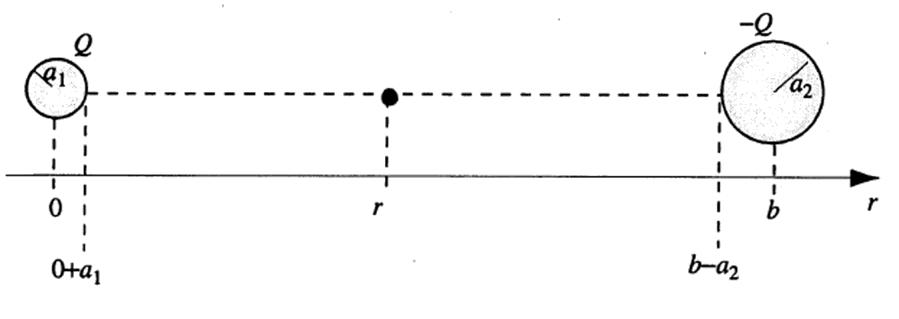
The potential difference between the spheres is given by
Note that Φ12 = Φ2 Φ1 is negative as expected, since the sphere labeled 1 is the one on which we placed positive charge. Based on our general definition of capacitance in (4.52) and in Figure 4.50 of the text (in which the conductor labeled 2 is that which has positive charge), the capacitance of this configuration is
from which we can find the resistance using RC = ϵ/σ as
which for b ≫a1, a2 reduces to
© 2015 Pearson Education, Inc., Hoboken, NJ. All rights reserved. This material is protected under all copyright laws as they currently exist. No portion of this material may be reproduced, in any form or by any means, without permission in writing from the publisher. 17 a a1 1 a 1 2
Figure 5.1 Figure for Problem 5.32
≫
Q E(r) = 4πϵ [ 1 r2 + (b 1 ] r)2
∫ (b a2) Q ∫ (b a2) [ 1 1 ] Φ12 = a1 Er(r)dr = 4πϵ a1 (b a2) r2 + dr (b r)2 = Q [ 1 1 ] 4πϵ r + b r = Q ( 1 + 1 1 1 ) 4πϵ a1 a2 b a1 b a2
Q C = Φ12
( 1 = 4πϵ a 1 1 + 2 b a1 1 ) b a2
1
1
1 R = 4πσ a +
1 b a1 1 ) b a2
( 1
© 2015 Pearson Education, Inc., Hoboken, NJ. All rights reserved. This material is protected under all copyright laws as they currently exist. No portion of this material may be reproduced, in any form or by any means, without permission in writing from the publisher. 17 a 1 ( 1 1 2) (a1 + a2) R ≃ 4πσ + a1 2 b ≃ 4πσa1a2
