USA - DOE_Review_of_Impacts_of_GHG_Emissions

A Critical Review of

Impacts of Greenhouse Gas Emissions on the U.S. Climate

Climate Working Group

United States Department of Energy

July 23, 2025

A Critical Review of Impacts of Greenhouse Gas Emissions on the U.S. Climate

Report to U.S. Energy Secretary Christopher Wright

July 23, 2025

Climate Working Group:

John Christy, Ph.D.

Judith Curry, Ph.D.

Steven Koonin, Ph.D.

Ross McKitrick, Ph.D.

Roy Spencer, Ph.D.

This report is being disseminated by the Department of Energy. As such, this document was prepared in compliance with Section 515 of the Treasury and General Government Appropriations Act for Fiscal Year 2001 (Public Law 106-554) and information quality guidelines issued by the Department of Energy.

Copyright © 2025 United States

Suggested citation:

Climate Working Group (2025) A Critical Review of Impacts of Greenhouse Gas Emissions on the U.S. Climate. Washington DC: Department of Energy, July 23, 2025

SECRETARY’S FOREWORD

Energy, Integrity, and the Power

of Human Potential

Over my lifetime, I’ve had the privilege of working as an energy entrepreneur across a range of fields nuclear, geothermal, natural gas, and more and I now serve as Secretary of Energy under President Donald Trump. But above all, I’m a physical scientist who sees modern energy as nothing short of miraculous. It powers every aspect of modern life, drives every industry, and has made America an energy powerhouse with the ability to fuel global progress.

The rise of human flourishing over the past two centuries is a story worth celebrating. Yet we are told relentlessly that the very energy systems that enabled this progress now pose an existential threat. Hydrocarbon-based fuels, the argument goes, must be rapidly abandoned or else we risk planetary ruin.

That view demands scrutiny. That’s why I commissioned this report: to encourage a more thoughtful and science-based conversation about climate change and energy. With my technical background, I’ve reviewed reports from the Intergovernmental Panel on Climate Change, the U.S. government’s assessments, and the academic literature. I’ve also engaged with many climate scientists, including the authors of this report.

What I’ve found is that media coverage often distorts the science. Many people walk away with a view of climate change that is exaggerated or incomplete. To provide clarity and balance, I asked a diverse team of independent experts to critically review the current state of climate science, with a focus on how it relates to the United States.

I didn’t select these authors because we always agree far from it. In fact, they may not always agree with each other. But I chose them for their rigor, honesty, and willingness to elevate the debate. I exerted no control over their conclusions. What you’ll read are their words, drawn from the best available data and scientific assessments.

I’ve reviewed the report carefully, and I believe it faithfully represents the state of climate science today. Still, many readers may be surprised by its conclusions which differ in important ways from the mainstream narrative. That’s a sign of how far the public conversation has drifted from the science itself.

To correct course, we need open, respectful, and informed debate. That’s why I’m inviting public comment on this report. Honest scrutiny and scientific transparency should be at the heart of our policymaking.

Climate change is real, and it deserves attention. But it is not the greatest threat facing humanity. That distinction belongs to global energy poverty. As someone who values data, I know that improving the human condition depends on expanding access to reliable, affordable energy. Climate change is a challenge not a catastrophe. But misguided policies based on fear rather than facts could truly endanger human well-being.

We stand at the threshold of a new era of energy leadership. If we empower innovation rather than restrain it, America can lead the world in providing cleaner, more abundant energy lifting billions out of poverty, strengthening our economy, and improving our environment along the way.

EXECUTIVE SUMMARY

This report reviews scientific certainties and uncertainties in how anthropogenic carbon dioxide (CO2) and other greenhouse gas emissions have affected, or will affect, the Nation’s climate, extreme weather events, and selected metrics of societal well-being. Those emissions are increasing the concentration of CO2 in the atmosphere through a complex and variable carbon cycle, where some portion of the additional CO2 persists in the atmosphere for centuries.

Elevated concentrations of CO2 directly enhance plant growth, globally contributing to “greening” the planet and increasing agricultural productivity [Section 2.1, Chapter 9]. They also make the oceans less alkaline (lower the pH). Thatis possibly detrimentalto coral reefs, although the recent rebound of the Great Barrier Reef suggests otherwise [Section 2.2]

Carbon dioxide also acts as a greenhouse gas, exerting a warming influence on climate and weather [Section 3.1]. Climate change projections require scenarios of future emissions. There is evidence that scenarios widely-used in the impacts literature have overstated observed and likely future emission trends [Section 3.1].

The world’s several dozen global climate models offer little guidance on how much the climate responds to elevated CO2, with the average surface warming under a doubling of the CO2 concentration ranging from 1.8°C to 5.7°C [Section 4.2] Data-driven methods yield a lower and narrower range [Section 4.3] Global climate models generally run “hot” in their description of the climate of the past few decades too much warming at the surface and too much amplification of warming in the lower- and midtroposphere [Sections 5.2-5.4]. The combination of overly sensitive models and implausible extreme scenarios for future emissions yields exaggerated projections of future warming.

Most extreme weather events in the U.S. do not show long-term trends. Claims of increased frequency orintensityofhurricanes,tornadoes,floods,anddroughtsarenotsupportedbyU.S.historicaldata[Sections 6.1-6.7]. Additionally, forest management practices are often overlooked in assessing changes in wildfire activity [Section 6.8]. Global sea levelhas risenapproximately 8 inches since 1900, but there are significant regional variations driven primarily by local land subsidence; U.S. tide gauge measurements in aggregate show no obvious acceleration in sea level rise beyond the historical average rate [Chapter 7].

Attribution of climate change or extreme weather events to human CO2 emissions is challenged by natural climate variability, data limitations, and inherent model deficiencies [Chapter 8]. Moreover, solar activity's contribution to the late 20th century warming might be underestimated [Section 8.3.1]

Both models and experience suggest that CO2-induced warming might be less damaging economically than commonly believed, and excessively aggressive mitigation policies could prove more detrimental than beneficial [Chapters 9, 10, Section 11.1]. Social Cost of Carbon estimates, which attempt to quantify the economic damage of CO2 emissions, are highly sensitive to their underlying assumptions and so provide limited independent information [Section 11.2].

U.S. policy actions are expected to have undetectably small direct impacts on the global climate and any effects will emerge only with long delays [Chapter 12].

PREFACE

This document originated in late March 2025 when Secretary Wright assembled an independent group to write a report on issues in climate science relevant for energy policymaking, including evidence and perspectives that challenge the mainstream consensus. We agreed to undertake the work on the condition that there would be no editorial oversight by the Secretary, the Department of Energy, or any other government personnel. This condition has been honored throughout the process and the writing team has worked with full independence.

The group began working in early April with a May 28 deadline to deliver a draft for internal DOE review.The shorttimeline and thetechnical nature of thematerialmeant that we could notcomprehensively review all topics. Rather, we chose to focus on topics that are treated by a serious, established academic literature; that are relevant to our charge; that are downplayed in, or absentfrom, recent assessment reports; and that are within our competence.

While the report is intended to be accessible to non-experts, we have omitted some introductory or explanatory material that can easily be accessed elsewhere. Nor have we attempted to survey the entire literature related to the topics covered. We have focused as much as possible on literature published since 2020 and referenced previous IPCC and NCA assessment reports. We have also used data through 2024 where possible.

The writing team is grateful to Secretary Wright for the opportunity to prepare this report and for his support of independent scientific assessment and open scientific debate We are also grateful to a team of anonymous DOE and national lab reviewers whose input helped improve the final report.

John Christy, Ph.D.

Judith Curry, Ph.D.

Steven Koonin, Ph.D.

Ross McKitrick, Ph.D.

Roy Spencer, Ph.D.

PART I: DIRECT HUMAN INFLUENCE ON ECOSYSTEMS AND THE CLIMATE

1 CARBON DIOXIDE AS A POLLUTANT

Chapter summary:

Carbon dioxide (CO2) differs in many ways from the so-called Criteria Air Pollutants. It does not affect local air quality and has no human toxicological implications at ambient levels. It is an issue of concern because of its effects on the global climate.

The Clean Air Actof 1970 defined six so-called Criteria Air Contaminants subject to regulation (EPA): particulate matter, ground-level ozone, sulfur dioxide, nitrogen dioxide, lead, and carbon monoxide. In 2007, the Supreme Court ruled that greenhouse gases (CO2 among them) were also “pollutants” subject to regulation under Clean Air Act (Mass. v. EPA, 2007). While the definition of “pollutant” is ultimately a legal matter, there are importantscientific distinctions between CO2 and the Criteria Air Contaminants. The latter are subject to regulatory control because they cause local problems depending on concentrations that include nuisances (odor, visibility), damage to plants, and, at high enough exposure levels, toxicological effects in humans. In contrast, CO2 is odorless, does not affect visibility and has no toxicological effects at ambient levels. It is a naturally occurring part of the atmosphere and a key component of human and plant respiration. CO2 is essential for plant photosynthesis and higher levels are beneficial for vegetation. In these aspects, CO2 is similar to water vapor.

Ambient outdoor air today contains about 430 parts per million (ppm) CO2, increasing at about 2 ppm per year. The U.S. Occupational Safety and Health Administration issues guidelines for indoor workplaces in which elevated CO2 might be encountered, such as where dry ice is used. The Permissible Exposure Limit is 5,000 ppm over 8 hours (OSHA, 2024). Allen et al. (2015) reported evidence of diminished performance on some cognitive tasks among workers in office cubicles when exposed to CO2 levels above 1,000-1,500 ppm. These levels are far larger than any plausible ambient outdoor value through the end of the 22nd century.

The growing amount of CO2 in the atmosphere directly influences the earth system by promoting plant growth (global greening), thereby enhancing agricultural yields, and by neutralizing ocean alkalinity. But the primary concern about CO2 is its role as a greenhouse gas (GHG) that alters the earth’s energy balance, warming the planet. How the climate will respond to that influence is a complex question that will occupy much of this report.

References

Allen, J., Macnaughton, P., Satish, U., et al. (2015). Associations of cognitive function scores with carbon dioxide, ventilation, and volatile organic compoundexposures in office workers:A controlledexposure study of green and conventional office environments. Environmental Health Perspectives. 124. https://doi.org/10.1289/ehp.1510037

Massachusetts v. Environmental Protection Agency, 549 U.S. 497 (2007). https://www.oyez.org/cases/2006/05-1120

U.S. Environmental Protection Agency. (n.d.). Criteria air pollutants. https://www.epa.gov/criteria-airpollutants

U.S. Occupational Safety and Health Administration. (2024). OSHA occupational chemical database: Carbon dioxide. https://www.osha.gov/chemicaldata/183

2

DIRECT IMPACTS OF CO2 ON THE ENVIRONMENT

Chapter summary:

CO2 enhances photosynthesis andimproves plantwater use efficiency, thereby promoting plant growth. Global greening due in part to increased CO2 levels in the atmosphere is well-established on all continents.

CO2 absorption in sea water makes the oceans less alkaline. The recentdecline in pH is within the range of natural variability on millennial time scales. Most ocean life evolved when the oceans were mildly acidic. Decreasing pH might adversely affect corals, although the Australian Great Barrier Reef has shown considerable growth in recent years.

2.1 CO2 as a contributor to global greening

The growing CO2 concentration in the atmosphere has the important positive effect of promoting plant growth by enhancing photosynthesis and improving water use efficiency. That is evident in the “global greening” phenomenon discussed below, as well as in the improving agricultural yields discussed in Chapter 10. Here we focus just on CO2 fertilization; research on combined effects due to temperature and precipitation changes are discussed in Chapter 10.

2.1.1 Measurement of global greening

“Greening” refers to an increase in the fraction of the Earth’s surface covered by plants. It can be quantified by the “Leaf Area Index” (LAI) measured by satellite. Many studies over the past decade have confirmed a global greening pattern (increase in LAI) attributable in part to rising CO2 levels. Zhu et al. (2016) was one of the firststudies to report that global greening was detectable using satellite sensors. From 1982 to 2011 they detected greening over 25-50 percent of the Earth versus “browning” over only four percent and attributed 70 percent of the greening to rising CO2 levels (see Figure 2.1). Other contributors included land-use changes, warming and nitrogen. The fraction attributable to CO2 was largest in the tropics; other factors played more dominant roles in CONUS

Zeng et al. (2017) confirmed the pattern of greening, noting thatover thirty years it had added 8 percent to global leaf area and that greening was mitigating warming. Greening has been observed globally. Chen et al. (2019) show that in China and India much of it is driven by land management changes. Thus, while China accounts for only 6.6 percent of global vegetatedarea it accounts for 25 percent of global netincrease in LAI. Piao et al. (2020) noted that greening was even observable in the Arctic. CO2 fertilization effects are influenced by local temperature and nutrient and water availability, all of which vary regionally.

While plant models predict increased photosynthesis in response to rising CO2, Haverd et al. (2020) reported a CO2 fertilization rate much larger than model predictions. That is, CO2 fertilization had driven an increase in observed global photosynthesis by 30 percent since 1900, versus 17 percent predicted by plant models. If true it would indicate that global models of the socioeconomic impacts of rising CO2 have understated the benefits to crops and agriculture Keenan et al (2023), however, estimated a lower fertilization rate more in line with models. The connection between CO2 fertilization and agriculture will be discussed in Chapter 9

Figure 2.1: Trends in average Leaf Area Index (LAI). Source: Zhu et al. 2016 Figure 3.

Piao et al. (2020) and Chen et al. (2024) report that the greening trend continues with no evidence of slowdown, and CO2 fertilization remains the dominant driver

2.1.2 Photosynthesis and CO2 levels

Plants build biomass through photosynthesis, a process that converts carbon dioxide, water, and light into sugar. The plant enzyme responsible for photosynthesis is Ribulose-1,5-bisphosphatecarboxylase/oxygenase or “Rubisco”. Photosynthesis is initiated when CO2 is available at the surface of the Rubisco enzyme where it is converted to a molecule with 3 carbon atoms and thereafter incorporated into plant mass. This is referred to as the “C3” process.

Rubisco is estimated to have evolved about 3 billion years ago. Over geological time the Earth’s atmospheric CO2 levels were usually many times higher than they are today About 400 million years ago CO2 levels were an estimated 2,000-4,000 ppm and were at or above 1,000 ppm for much of the interval from 200 to 50 million years ago (Berner 2006, Judd et al. 2024). Over the past 35 million years the level of atmospheric CO2 has been steadily declining, falling to as low as 170 ppm during glaciations (Gerhart and Ward 2010). While the modern rate of change in CO2 may be high compared to prior intervals, the geological evidence is that plants and animals evolved under much higher CO2 levels than at present.

In response to low-CO2 conditions some plants evolved another photosynthetic pathway called C4, in which CO2 is concentrated in the vicinity of Rubisco, allowing for the C3 process to function more efficiently. For agricultural purposes the plant categories are:

• C3: rice, wheat, soybeans and most other crops

• C4: maize (corn), sugar cane, millet, sorghum

Had atmospheric CO2 levels continued declining, plant growth would have declined and eventually ceased. Below 180 ppm, the growth rates of many C3 species are reduced 40-60 percent relative to 350 ppm (Gerhart and Ward 2010) and growth has stopped altogether under experimental conditions of 60 140 ppm CO2. Some C4 plants are still able to grow at levels even as low as 10 ppm, albeit very slowly (Gerhart and Ward 2010).

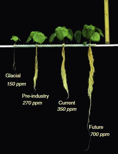
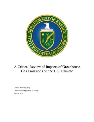
Figure 2.2: growth of Abutilon theophrasti after 14 days under identical conditions but for the indicated variations in CO2 levels. Source: Gerhart and Ward (2010). Note “Current” corresponds to 1988 in image.

Current CO2 levels are about 430 ppm, up from 280 ppm in the early 1800s. The positive response of plants to extra CO2 is illustrated in Figure 2.2, reproduced from Gerhart and Ward (2010). It shows the growth effect of CO2 on Velvetleaf (Abutilon theophrasti) seedlings over 14 days under controlled conditions where only the CO2 exposure is varied. The gains induced by increasing CO2 from 150 ppm to 350 ppm continue under a further doubling to 700 ppm.

Over the past 60+ years there have been thousands of studies on the response of plants to rising CO2 levels. The overwhelming theme is that plants, especially C3 plants, benefit from extra CO2. There are two mechanisms by which CO2 confers a growth benefit:

• Enhanced photosynthesis via the metabolic pathways described above.

• Increased water use efficiency. This arises because plants draw in CO2 by opening the stomata (pores) on the leaf surface. When CO2 is scarce the stomata must be kept wide open for long periods, allowing water to evaporate. Under enriched CO2 conditions the stomata remain closed for longer periods, thus helping the plant retain water longer, and so increasing water use efficiency.

Specific effects of climate change on U.S. agriculture will be reviewed in Chapter 9.

2.1.3

Rising CO2 and crop water use efficiency

Derying et al. (2016) surveyed evidence on crop water productivity (CWP), the yield per unit of water used, drawing attention to the potential for CO2 both to enhance photosynthesis and to reduce leaf-level transpiration (water loss during leaf respiration). They surveyed all available FACE data (Free Air CO2 Enrichment seeChapter9)oncropyieldchangesformaize(corn),wheat,rice,andsoybeanandcombined it with crop modeldata simulating yield responses as of 2080 under the extreme RCP8.5 emissions scenario in four growing regions (Tropics, Arid, Temperate and Cold) each of which were split into rainfed and irrigated sub-regions. They reported that models without CO2 fertilization predicted CWP losses in every region, but those were more than offset by CO2 fertilization so that all regions showed a net CWP gain. Deryng et al. (2016) also reported that negative impacts of warming on wheat and soybean yields were fully offset by CWP gains and mitigated by up to 90 percent for rice and 60 percent for maize.

Similarly, Cheng et al. (2017) noted that increased Gross Primary Production from 1982 to 2011 due to rising CO2 uptake was accompanied by such large gains in CWP that global water use by plants had not increased, despite the extra biomass

Deryng et al. (2016) assumed that climate change would “exacerbate water scarcity”. Yet while models do predict that drylands will expand under climate warming, current data show the opposite: greening is happening even in arid areas. Zhang et al. (2024) report that due to increased CO2 levels “increasing aridity in drylands won’t lead to a general loss of vegetation productivity”; at most only 4 percent of currently arid areas will see increased desertification.

2.1.4

CO2 fertilization benefits in IPCC Reports

The IPCC has only minimally discussed global greening and CO2 fertilization of agricultural crops. The topic is briefly acknowledged in a few places in the body of the IPCC 6th and earlier Assessment Reports but is omitted in all Summary documents. Section 2.3.4.3.3 of the AR6 Working Group I report, entitled “global greening and browning,” points out that the IPCC Special Report on Climate Change and Land had concluded with high confidence that greening had increased globally over the past 2-3 decades. It then discusses that there are variations in the greening trend among data sets, concluding that while they have high confidence greening has occurred, they have low confidence in the magnitude of the trend. There are also brief mentions of CO2 fertilization effects and improvements in water use efficiency in a few other chapters in the AR6 Working Groups I and II Reports.

Overall, however, the Policymaker Summaries, Technical Summaries, and Synthesis Reports of AR5 and AR6 do not discuss the topic.

2.2 The Alkaline Oceans

2.2.1

Changing pH

A neutral aqueous solution has a pH of 7.0, while one with pH greater than 7.0 is alkaline (also termed basic) and with pH less than 7.0 is acidic. The modern-day global average pH of surface sea water is estimated to be 8.04 (Copernicus Marine Service 2025, Figure 2.3), down from an estimated value of 8.2 in pre-Industrial times (Gattuso and Hansson, 2011). As CO2 concentrations in the atmosphere increased, the oceans absorbed more, which decreases their pH. Depending upon the oceans’ buffering capacity, they are expected to become somewhat less alkaline over time, consistent with the observed decrease in pH.

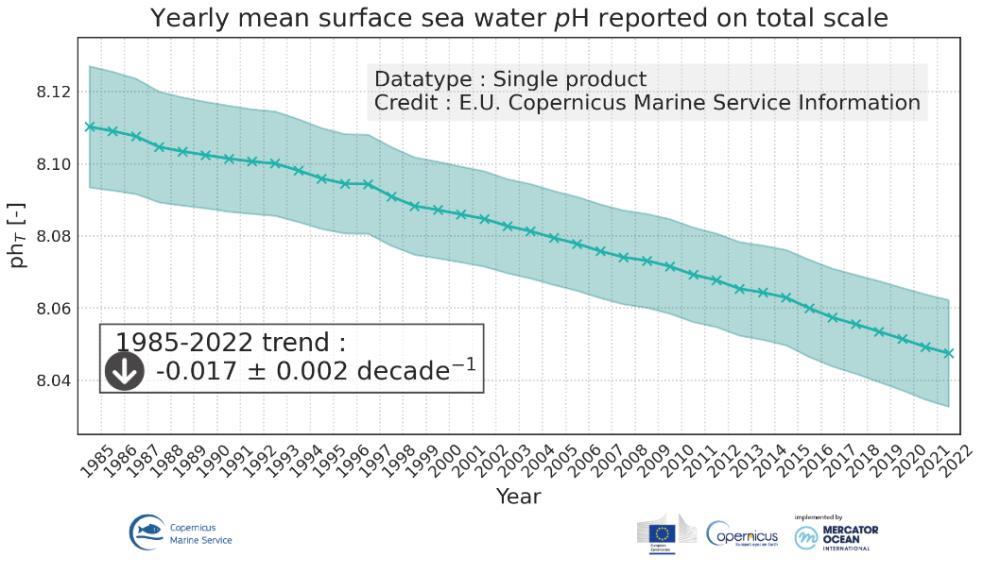
Figure 2.3: Ocean pH 1985 – 2022. Source: Copernicus Marine Service 2025

While this process is often called “ocean acidification”, that is a misnomer because the oceans are not expected to become acidic; “ocean neutralization” would be more accurate. Even if the water were to turn acidic, it is believed that life in the oceans evolved when the oceans were mildly acidic with pH 6.5 to 7.0 (Krissansen-Totton et al., 2018). On the time scale of thousands of years, boron isotope proxy measurements show that ocean pH was around 7.4 or 7.5 during the last glaciation (up to about 20,000 years ago) increasing to present-day values as the world warmed during deglaciation (Rae et al., 2018). Thus, ocean biota appear to be resilient to natural long-term changes in ocean pH since marine organisms were exposed to wide ranges in pH.

2.2.2 Coral reef changes

There are concerns that a decreasing pH of sea water will reduce the calcification rate of coral reefs. But coral reefs already endure large swings in pH, partly due to daily photosynthetic activity in the reef; measured pH values range from 9.4 during the day to 7.5 at night (Revelle and Fairbridge, 1957). De’ath et al. (2009) reported that a portion of Australia’s Great Barrier Reef (GBR, the world’s largest coral reef ecosystem) hadexperienced a 14 percent decline in calcification since 1990. This was tentatively attributed to increasing water temperature and decreasing pH. But Ridd et al. (2013) showed that report to have resulted from a biased data analysis that, when corrected, showed no change in calcification rates. Nevertheless, the alarm produced by the original paper has persisted as evidenced by the large number of published citations (541) to the originalstudy compared to only 11 citations to the correction (as of 30 April 2025).

The most recent annual summary of GBR conditions from the Australian Institute of Marine Science indicates that coral production has rebounded strongly (AIMS, 2023). Figure 2.4 shows the results of the AIMS surveys of hard coral cover, expressed as a percentage of the reef area. Much of the decline in the GBR before 2011 turned out to be due to intense tropical cyclone activity (Beeden et al., 2015) as well as a string of marine heatwaves, agricultural runoff and invasive species (Woods Hole, 2023). Given the reported declines in GBR calcification between 1990 and 2009 and the continued increase in atmospheric CO2 levels, the rebound has surprised some observers.

Figure 2.4 Hard coral cover of three regions of the Great Barrier Reef 1985 to 2023. Source: AIMS 2023.

It is being increasingly recognized that publication bias (alarming ocean acidification results preferred by high-impact research publications) exaggerates the reported impacts of declining ocean pH. An ICES Journal of Marine Science Special Issue addressed this problem with an article entitled, Towards a Broader Perspective on Ocean Acidification Research. In the Introduction to that Special Issue, H. I. Browman stated, “As is true acrossall of science, studies that report no effect of ocean acidification are typically more difficult to publish.” (Browman, 2016).

Similarly, a meta-analysis (Clements et al., 2021) of the negative effects of ocean acidification on reef fish behavior found what they called a “decline effect”: initially dramatic conclusions published in prominent journals showing apparently large impacts of acidification tended to be followed up by subsequent studies on larger sample sizes yielding much smaller and typically non-existent effects. They call for their colleagues to improve research practices to counter the “decline effect”:

[The] vast majority of studies with large effect sizes in this field tend to be characterized by low sample sizes, yet are published in high-impact journals and have a disproportionate influence on the field in terms of citations. We contend that ocean acidification has a negligible direct impact on fish behavior, and we advocate for improved approaches to minimize the potential for a decline effect in future avenues of research (Clements et al., 2021)

In summary, ocean life is complex and much of it evolved when the oceans were acidic relative to the present. The ancestors of modern coral firstappeared about 245 million years ago CO2 levels for more than 200 million years afterward were many times higher than they are today. Much of the public discussion of the effects of ocean “acidification” on marine biota has been one-sided and exaggerated.

References

AR6: Intergovernmental Panel on Climate Change Sixth Assessment Report (2021) Working Group I Contribution. www.ipcc.ch.

Australian Institute of Marine Science. (2022). Continued coral recovery leads to 36-year highs across two-thirds of the Great Barrier Reef. https://www.aims.gov.au/sites/default/files/202208/AIMS_LTMP_Report_on%20GBR_coral_status_2021_2022_040822F3.pdf

Beeden, R., Maynard, J., Puotinen, M., Marshall, P., Dryden, J., Goldberg, J., and Williams, G. (2015). Impacts and recovery from Severe Tropical Cyclone Yasi on the Great Barrier Reef. PLOS ONE, 10, e0121272. https://doi.org/10.1371/journal.pone.0121272

Berner, R. A. (2006). GEOCARBSULF: A combined model for Phanerozoic atmospheric O₂ and CO₂. Geochimica et Cosmochimica Acta, 70, 5653–5664.

Browman, H. I. (2016). Applying organized scepticism to ocean acidification research. ICES Journal of Marine Science, 73(3), 529.1–536. https://doi.org/10.1093/icesjms/fsw010

Chen, C., Park, T., Wang, X., Piao, S., Xu, B., Chaturvedi, R. K., and Myneni, R. B. (2019). China and India lead in greening of the world through land-use management. Nature Sustainability, 2, 122–129. https://www.nature.com/articles/s41893-019-0220-7

Chen, X., Wang, Y., Liu, Y., and Piao, S. (2024). The global greening continues despite increased drought stress since 2000. Global Ecology and Conservation, 49, e02791. https://www.sciencedirect.com/science/article/pii/S2351989423004262

Cheng, L., Zhang, L., Wang, Y. P., et al. (2017). Recent increases in terrestrial carbon uptake at little cost to the water cycle. Nature Communications, 8, 110. https://doi.org/10.1038/s41467-017-00114-5

Clements, J. C., Sundin, J., Clark, T. D., and Jutfelt, F. (2022). Meta-analysis reveals an extreme “decline effect” in the impacts of ocean acidification on fish behavior. PLOS Biology, 20(2), e3001511. https://doi.org/10.1371/journal.pbio.3001511

Copernicus Marine Service. (2025). Global ocean acidification – Mean sea water pH time series and trend from multi-observations reprocessing. https://data.marine.copernicus.eu/product/GLOBAL_OMI_HEALTH_carbon_ph_area_averaged/desc ription

De’ath, G., Lough, J., and Fabricius, K. (2009). Declining coral calcification on the Great Barrier Reef. Science, 323, 116–119. https://doi.org/10.1126/science.1165283

Deryng, D., Conway, D., Ramankutty, N., Price, J., Warren, R., Jones, R., ... and Elliott, J. (2016). Regional disparities in the beneficial effects of rising CO₂ concentrations on crop water productivity. Nature Climate Change. https://doi.org/10.1038/nclimate2995

Gattuso, J. P., and Hansson, L. (Eds.). (2011). Ocean acidification: Background and history. Oxford University Press.

Gerhart, L. M., and Ward, J. K. (2010). Plant responses to low [CO₂] of the past. New Phytologist, 188, 674–695. https://nph.onlinelibrary.wiley.com/doi/pdf/10.1111/j.1469-8137.2010.03441.x

Haverd, V., B. Smith, J. G. Canadell, et al. (2020). Higher than expected CO₂ fertilization inferred from leaf to global observations. Global Change Biology, 26, 2390–2402. https://doi.org/10.1111/gcb.14950

Keenan, T. F., X. Luo, B. D. Stocker, et al. (2023). A constraint on historic growth in global photosynthesis due to rising CO2. Nature Climate Change 13(12): 1376-1381 DOI: 10.1038/s41558023-01867-2.

Judd, E. J., Scotese, C. R., Young, S. A., et al. (2024). A 485-million-year history of Earth’s surface temperature. Science, 385(6715). https://doi.org/10.1126/science.adk3705

Krissansen-Totton, J., Arney, G. N., and Catling, D. C. (2018). Constraining the climate and ocean pH of the early Earth with a geological carbon cycle model. Proceedings of the National Academy of Sciences, 115(6), 4105–4110. https://doi.org/10.1073/pnas.1721296115

Piao, S., X. Wang, T. Park, et al. (2020). Characteristics, drivers and feedbacks of global greening. Nature Reviews Earth & Environment 1(1): 14-27 DOI: 10.1038/s43017-019-0001-x

Rae, J. W. B., Burke, A., Robinson, L. F., et al. (2018). CO₂ storage and release in the deep Southern Ocean on millennial to centennial timescales. Nature, 562, 569–573. https://doi.org/10.1038/s41586018-0614-0

Revelle, R., and Fairbridge, R. W. (1957). Carbonate and carbon dioxide. In J. W. Hedgpeth (Ed.), Treatise on marine ecology and paleoecology (Vol. 1). Geological Society of America.

Ridd, P., Silva, E., and Stieglitz, T. (2013). Have coral calcification rates slowed in the last twenty years? Marine Geology, 346, 392–399. https://doi.org/10.1016/j.margeo.2013.09.002

Woods Hole Oceanographic Institution. (2023). Is the Great Barrier Reef making a comeback? https://www.whoi.edu/oceanus/feature/is-the-great-barrier-reef-making-a-comeback/ Zeng, Z., Piao, S Li, L., et al. (2017). Climate mitigation from vegetation biophysical feedbacks during the past three decades. Nature Climate Change https://doi.org/10.1038/nclimate3299

Zhang, Y., Liu, Y., Chen, X., et al. (2024). Less than 4% of dryland areas are projected to desertify despite increased aridity under climate change. Nature Communications Earth and Environment, 5. https://www.nature.com/articles/s43247-024-01463-y

Zhu, Z., Piao, S., Myneni, R. B., et al. (2016). Greening of the Earth and its drivers. Nature Climate Change, 6, 791–795. https://www.nature.com/articles/nclimate3004

3 HUMAN INFLUENCES ON THE CLIMATE

Chapter Summary:

The global climate is naturally variable on all time scales. Anthropogenic CO2 emissions add to that variability by changing the total radiative energy balance in the atmosphere.

The IPCC has downplayed the role of the sun in climate change but there are plausible solar irradiance reconstructions that imply it contributed to recent warming.

Climate projections are based on IPCC emission scenarios that have tended to exceed observed trends. Mostacademic climate impactstudies in recent years are based upon the extreme RCP8.5 scenario that is now considered implausible; its use as a business-as-usual scenario has been misleading.

Carbon cycle models connect annual emissions to growth in the atmospheric CO2 stock. While models disagree over the rate of land and ocean CO2 uptake, all agree that it has been increasing since 1959. There is evidence that urbanization biases in the land warming record have not been completely removed from climate data sets.

3.1 Components of radiative forcing and their history

3.1.1 Historical radiative forcing

A changing climate has been the norm throughout the Earth’s 4.6-billion-year history. The Earth’s temperature and weather patterns change naturally over timescales ranging from decades to millions of years. Natural variations in the surface climate originate in two ways. Internal climate fluctuations associated with circulations in the atmosphere and ocean exchange energy, water, and carbon between the atmosphere,oceans,land,andice.Externalinfluencesontheclimatesystemincludevariationsintheenergy received from the sun and the effects of volcanic eruptions. Human activities influence climate through changing land use and land cover. Humans are also changing the composition of the atmosphere by emissions of CO2 and other greenhouse gases and by altering the concentration of aerosol particles in the atmosphere.

The earth is warmed by the sunlight it absorbs and is cooled by the heat it radiates to space. Averaged over the Earth’s surface, each of these processes involve power flows of about 240 Watts per square meter (W/m2). When they are in balance, there are no net external causes of warming or cooling. Both human and natural influences on the climate alter this balance and so cause the climate to change.

Influences on the Earth’s energy balance at the top of the atmosphere are quantified by “radiative forcing”, the extent to which they disturb the warming/cooling balance; a positive forcing warms while a negative forcing cools. The IPCC’s estimated history of major components of radiative forcing since 1750 is shown in the following two figures from its AR6.

Figure 3.1.1: IPCC estimates of radiative forcing components over time. Shading indicates uncertainty ranges. Source: AR6 WGI Ch2 Fig. 10

Figure 3.1.2 IPCC estimates of radiative forcing component changes from 1750 to 2019. Source: AR6 WGI Ch 7 Fig. 7-6.

These graphs show that the total radiative forcing is comprised of both natural and anthropogenic components. Carbon dioxide is the largest human influence on the climate and the one most relevant to the influence of fossil fuel use. It exerts a warming influence by decreasing the cooling power of the atmosphere. Emissions of CO2 are accumulating in the atmosphere, as described in the following section, so that the warming influence is growing. Other greenhouse gases (methane, nitrous oxide, halogens, and ozone) act similarly, currently adding another 75 percent to CO2’s warming. Aerosols exert an overall cooling effect, although with large uncertainties in the way they catalyze the formation of reflective clouds. As a result, understanding the causes of recent warming requires not just identifying the warming effects of CO2, but also the more uncertain cooling effects of aerosols.

The IPCC assesses the change in the radiative forcing by the sun to be negligible, based on their preference for data reconstructions thatimply minimal solar change since preindustrial times. But Connolly et al. (2021) reviewed sixteen different Total Solar Irradiance (TSI) reconstructions in the literature

covering the years 1600-2000; the reconstructions vary from almost no change in TSI to a relatively large upward trend. Those authors note that the variation in TSI reconstructions combined with variations in surface temperature reconstructions allows for inferences consistent with either no or most 20th century warming being attributable to the sun.

A particularly thorny issue is the gap in TSI data between 1989 and 1991 due to a delay in the launch of a monitor following the Space Shuttle Challenger disaster on January 28 1986. This delay prevented a replacement satellite from being launched in time to overlap with, and its readings to be intercalibrated with, the prior system (Zacharias 2014, Scafetta et al. 2019). This is called the ACRIM (Active Cavity Radiometer Irradiance Monitor) gap problem. The question of whether there is an upward trend in TSI over 1978 to 2018 hangs on how the ACRIM data gap is filled. Connolly et al. (2021) found that the IPCC’s consensus statements on solar forcing were formulated prematurely through the suppression of dissenting scientific opinions.

Another natural radiative forcing component is volcanic aerosols, which exert an episodic cooling influence. Box 4.1 in the IPCC AR6 Report addresses the climate impact of volcanic eruptions, noting three explosive volcanic eruptions that occurred in the first half of the 19th century. This included the 1815 Tambora eruption that resulted in the ‘year without summer’, with multiple harvest failures across the Northern Hemisphere. There is uncertainty about the sign of the relatively small forcing due to the submarine volcano Hunga Tonga which erupted in 2022 (Jenkins et al. 2023, Schoeberl et al. 2024)

Figure 3.1.1 shows that the anthropogenic forcing component was negligible before about 1900 and has increased steadily since, rising to almost 3 W/m2 today. However, this is still only about 1 percent of the unperturbed radiation flows, making it a challenge to isolate the effects of anthropogenic forcing; stateof-the-art satellite estimates of global radiative energy flows are only accurate to a few W/m2 .

Natural sources of global energy imbalance other than volcanoes and total solar irradiance (TSI) are not included in these graphs because they remain largely unknown.

3.1.2 Change in atmospheric CO2 since 1958

Carbon dioxide’s warming influence depends on how much “extra” CO2 accumulates in the atmosphere- i.e., its concentration above the preindustrial value of 280 ppm. The CO2 level as recorded at the Mauna Loa observatory in Hawaii, generally used as the representative global average concentration, is available online at https://gml.noaa.gov/ccgg/trends/index.html. The concentration was about 316 ppm at the start of the record in 1959 and is now about 430 ppm, a 36 percent increase. At the end of the last glaciation CO2 levels had fallen to about 180 ppm. As discussed in Chapter 2, C3 plants begin dying at CO2 levels below about 140 ppm and C4 plants at levels below 100 ppm, so if CO2 levels had continued falling plant life would have been imperiled.

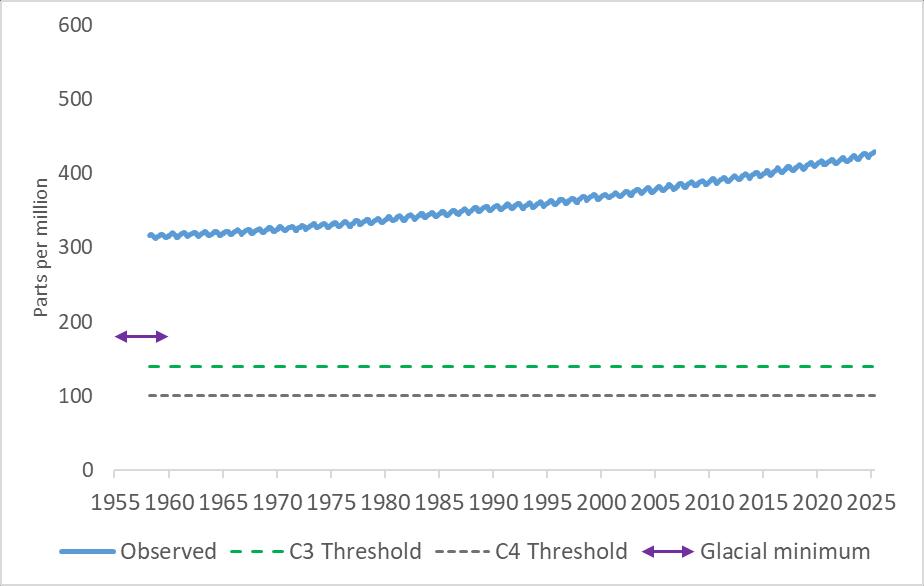
Fig. 3.1.3 Yearly average atmospheric CO2 concentrations (1959-2025) in ppm measured at Mauna Loa (blue). C3 Threshold: Level below which C3 plants begin dying (140 ppm, see Chapter 2). C4 Threshold: Level below which C4 plants begin dying (100 ppm, see Chapter 2). Glacial minimum: Minimum level during recent glaciations (purple arrow) CO2 data source: https://gml.noaa.gov/ccgg/trends/index.html

The annual increase in concentration is only about half of the CO2 emitted because land and ocean processes currently absorb “excess” CO2 at a rate approximately 50 percent of the human emissions. Future concentrations, and hence future human influences on the climate, therefore depend upon two components: (1) future rates of global human CO2 emissions, and (2) how fastthe land and ocean removeextra CO2 from the atmosphere. We discuss each of these in turn.

3.2 Future emission scenarios and the carbon cycle

3.2.1 Emission

scenarios

Assessing the dangers of future GHG emissions requires assumptions about what those emissions will be. Future emissions, and hence human influences on the climate, will depend upon future demographics, economic activity, regulation, and energy and agricultural technologies. Various assumptions about each of those lead to projections of greenhouse gas emissions and concentrations, aerosol concentrations, and changes in land use, which ultimately can be combined into assumptions about anthropogenic radiative forcing.

The great uncertainties about these many factors make it impossible to precisely predict future emissions. Instead, the IPCC has used various sets of scenarios meant to span a plausible range of possibilities for population, economy, and technologies. Recent versions of the scenarios are labeled by a number indicating the anthropogenic radiative forcing expected in 2100 under that scenario. Thus, a scenario labeled with a “6” corresponds to 6 W/m2 of human-induced radiative forcing (warming) at the end of the century. (Recall current anthropogenic radiative forcing is about 2.7 W/m2.)

Although the IPCC does not claim its emission scenarios are forecasts, they are often treated as such. Comparisonsofpastscenariogroupsagainstobservationsshow thatIPCCemission projectionshavetended to overstate actual subsequent emissions. For the IPCC Third and Fourth Assessment Reports a set of emission projections from the Special Report on Emission Scenarios was used; these were referred to as the SRES scenarios. McKitrick et al. (2012) showed that, when converted to per capita values, the SRES scenario emissions distribution was skewed upwards compared with observed trends. The bias of the SRES scenarios was confirmed by the later analysis of Hausfather et al. (2019) who showed that observed atmospheric CO2 concentrations tracked the low end of the SRES range and also of subsequent IPCC scenario ranges (Figure 3.2.1)

For AR5 the IPCC developed a new set of scenarios called the Representative Concentration Pathways (RCPs). These were identified by a number representing the increase in forcing and were thus called RCP2.6, RCP4.5, RCP6.0 and RCP8.5. RCP2.6 (implying an anthropogenic radiative forcing in 2100 of 2.6 W/m2) describes a GHG concentration pathway leading to warming well below 2°C. At the other end of the scale RCP8.5 is an extreme outcome implying nearly 5°C warming from 1900 to 2100.

RCP8.5 came to be referred to as the no-policy baseline, or “business-as-usual” scenario in both the academic literature and popular media. It was therefore used to generate the reference outcome supposedly representing the 21st century world in the absence of increasingly stringent emission reduction policies. But RCP8.5 was intended as a low-probability high emissions scenario and its use as a business-as-usual baseline has been criticized as grossly misleading.1 Hausfather and Peters (2020a) writing in a commentary in Nature, pointed out that RCP8.5 was developed as an extreme worst-case, and its misuse as a “business as usual” baseline has resulted in a large number of misleading studies and media reporting

The implausibility of the RCP8.5 scenario was examined by Burgess et al. (2021). The implausibility of RCP8.5 should not be interpreted as very unlikely (e.g. 95th percentile) or a “worst case”, but rather as genuinely implausible owing to the implausibility of the inputs required to reach a forcing of 8.5 W/m2 . They noted that RCP8.5 has already diverged from observed trends in energy use and the near future trends diverge sharply from those of the International Energy Agency (IEA), which provides market-based projections of energy use for the coming decades. Pielke Jr. et al (2022) further showed that the historic and projected IEA trends run near the bottom of the envelopes of both RCP projections and the more recent Shared Socioeconomic Pathway (SSP) scenario trends.

Schwalm et al. (2020) defended the use of RCP8.5 on the grounds that cumulative CO2 emissions over 2005-2020 track it more closely than the lower RCP scenarios. They also argue that a modified version of the IEA scenarios closely track RCP8.5 in the coming decades. Hausfather and Peters (2020b) responded that the skill of RCP8.5 over those 15 years is due to offsetting errors in its representation of CO2 from fuel use and land use change, and the apparent agreement with IEA in coming decades is due to Schwalm et al. adding in very high land use emissions. The IEA’s own projected CO2 emissions track well below RCP8.5.

Widespread use of RCP8.5 as a no-policy baseline has created a bias towards alarm in the climate impacts literature.Theextent of this problemwas confirmed in a literatureanalysis by Pielke Jr.and Ritchie (2020). They found that some 16,800 scientific papers published between 2010 and 2020 used the RCP8.5 scenario, with about 4,500 of the articles linking RCP8.5 to the concept of “business-as-usual”. Their analysis showed how RCP8.5 was misused not only by individual researchers, but also by influential science agencies like the IPCC and the U.S. National Climate Assessment (USNCA), which has directly led to misleading coverage in prominent media outlets.

1 This extreme scenario is useful for modelers, since a large forcing generates a large response (warming) making it easier to assess a model’s sensitivity. But that’s very different than claiming it is a plausible future outcome

Figure 3.2.1 Since the 1970s successive families of emission and concentration projections (colored lines) have consistently overestimated observations (black line). Source: Hausfather et al. (2019) Figure S4.

Pielke and Ritchie (2020) reported new studies using RCP8.5 were published at a rate of about 20 per day, with about two per day specifically linking RCP8.5 and “business as usual.” They conclude that the climate research community has spent a decade “committing scientific resources to science fiction” and that “The scientific literature has become imbalanced in an apocalyptic direction.”

The IPCC developed a new set of scenarios for AR6, the “Shared Socioeconomic Pathway” (SSP) scenarios, which have continued the bias shown in the RCP and SRES scenarios. Figure 3.2.2 shows total global observed CO2 emissions compiled by the International Energy Agency (IEA) merged with the emission projection from the EIA taking account of energy use projections and current policies. The other lines show the range of IPCC SSP scenarios (SSP1-SSP5). As of 2023, global CO2 emissions have been tracking well below SSP7.0 and are even below SSP2-4.5.

Figure 3.2.2. Observed and projected CO2 emissions. Source: IPCC (SSP scenarios) and Energy Information Administration (EIA). Green: observed historical emissions and EIA projections. Other lines: SSP1-5. Data source: Friedlingstein et al. (2024).

3.2.2 The carbon cycle relating emissions and concentrations

Carbon dioxide emissions from fossil fuel burning (and to a lesser extent deforestation and cement production) have led to steadily increasing CO2 concentrations in the atmosphere, as shown in Fig. 3.1.3. The relation between emissions and concentration is determined by the global carbon cycle of land and ocean processes that exchange carbon with the atmosphere. Our understanding of these processes was reviewed by Crisp et al. (2021).

There are about 850 Gt of carbon (GtC) in the Earth’s atmosphere2, almost all of it in the form of CO2. Each year, biological processes (plant growth and decay) and physical processes (ocean absorption and outgassing) exchange about 200 GtC of that carbon with the Earth’s surface (roughly 80 GtC with the land and 120 GtC with the oceans). Before human activities became significant, removals from the atmosphere were roughly in balance with additions. But burning fossil fuels (coal, oil, and gas) removes carbon from the ground and adds it to the annual exchange with the atmosphere. That addition (together with a much

2 Because CO2 is chemically transformed through the course of the carbon cycle, it is more convenient to track atoms of carbon rather than molecules of CO2. One gigatonne of carbon (GtC) is equivalent to about 3.7 Gt of CO2

smaller contribution from cement manufacturing) amounted to 10.3 GtC in 2023, or only about 5 percent of the annual exchange with the atmosphere.

The carbon cycle accommodates about 50 percent of humanity’s small annual injection of carbon into the air by naturally sequestering it through plant growth and oceanic uptake, while the remainder accumulates in the atmosphere (Ciais et al., 2013). For that reason, the annual increase in atmospheric CO2 concentration averages only about half of that naively expected from human emissions.

To project future CO2 concentrations in the atmosphere, and hence future human influences on the climate, it is important to know how the carbon cycle might change in the future. The historical near constancy of that 50 percent fraction means that the more CO2 humanity has produced, the faster nature removed it from the atmosphere. That 50 percent fraction changes somewhat from year to year due to natural carbon cycle imbalances from El Nino, La Nina, and varying weather patterns. There was also a substantialadditional reduction in atmospheric CO2 after the 1991 eruption of Mt. Pinatubo, a curious result that has yet to be explained (Angert et al., 2004).

The main processes that remove excess CO2 from the atmosphere are increased growth of land vegetation (especially at high latitudes), some increase in the sequestering of carbon in soils, and uptake of CO2 by the ocean due to the increasing partial pressure of atmospheric CO2 over that of CO2 dissolved in the ocean. All twenty land carbon cycle models tracked by the Global Carbon Project (Friedlingstein et al., 2024) show land processes have been removing excess CO2 at an increasing rate since 1959. This is consistent with a “global greening” phenomenon (Chapter 2.1) observed by satellites since monitoring of global greenness began in 1982.

While land vegetation has been responding positively to more atmospheric CO2, uptake of extra CO2 by ocean biological processes remains too uncertain to be measured reliably. Our current understanding of these and many more carbon cycle processes was reviewed by Crisp et al. (2021).

CO2 uptake by land processes

The uptake of extra CO2 from the atmosphere by land surface processes (as also inferred from global greening) has been modeled with 20 different dynamic global vegetation models, the outputs of which are updated every year by the Global Carbon Project (Friedlingstein, 2024). As seen in Fig. 3.2.3, all of those models agree thatvegetation and soils have been sequestering carbon from the atmosphere. But we also see that the long-term trends over 1959 to 2023 (65 years) vary widely between models, by nearly a factor of 7. This demonstrates that there remains considerable uncertainty in how fast land processes are removing CO2 from the atmosphere, which in turn creates uncertainty in future atmospheric CO2 concentrations, which then produce uncertainty in climate model simulations of future climate change.

Figure 3.2.3 Trends of annual CO2 uptake (GtCO2 per year per decade) by land processes during 1959-2023 simulated by 20 different dynamic global vegetation models periodically reported by the Global Carbon Project (Friedlingstein, 2024).

CO2 uptake by ocean processes

The uptake of extra CO2 from the atmosphere by ocean processes has been modeled with 10 different ocean biogeochemistry models, the outputs of which are updated every year by the Global Carbon Project (Friedlingstein, 2024). Like the results from the land models, all of the ocean models agree that the global oceans have been sequestering carbon from the atmosphere at an increasing rate during 1959-2023 (Fig. 3.2.4). Unlike the land models, however, the ocean models show much better agreement with each other, with the model producing the fastest increasing CO2 uptake being only 65 percent faster than the model withthemostslowly increasingCO2 uptake.Inspiteofthe relativeagreementamongmodels,Friedlingstein et al. (2022) notes that there is substantial discrepancy between the different methods on the strength of the ocean sink over the last decade, particularly in the Southern Ocean.

Note that the average trend in CO2 uptake across all land models in Fig. 3.2.3 is 25 percent larger than the average trend in ocean uptake. This suggests land processes are increasing in their ability to remove CO2 faster than ocean processes are increasing their CO2 sequestration.

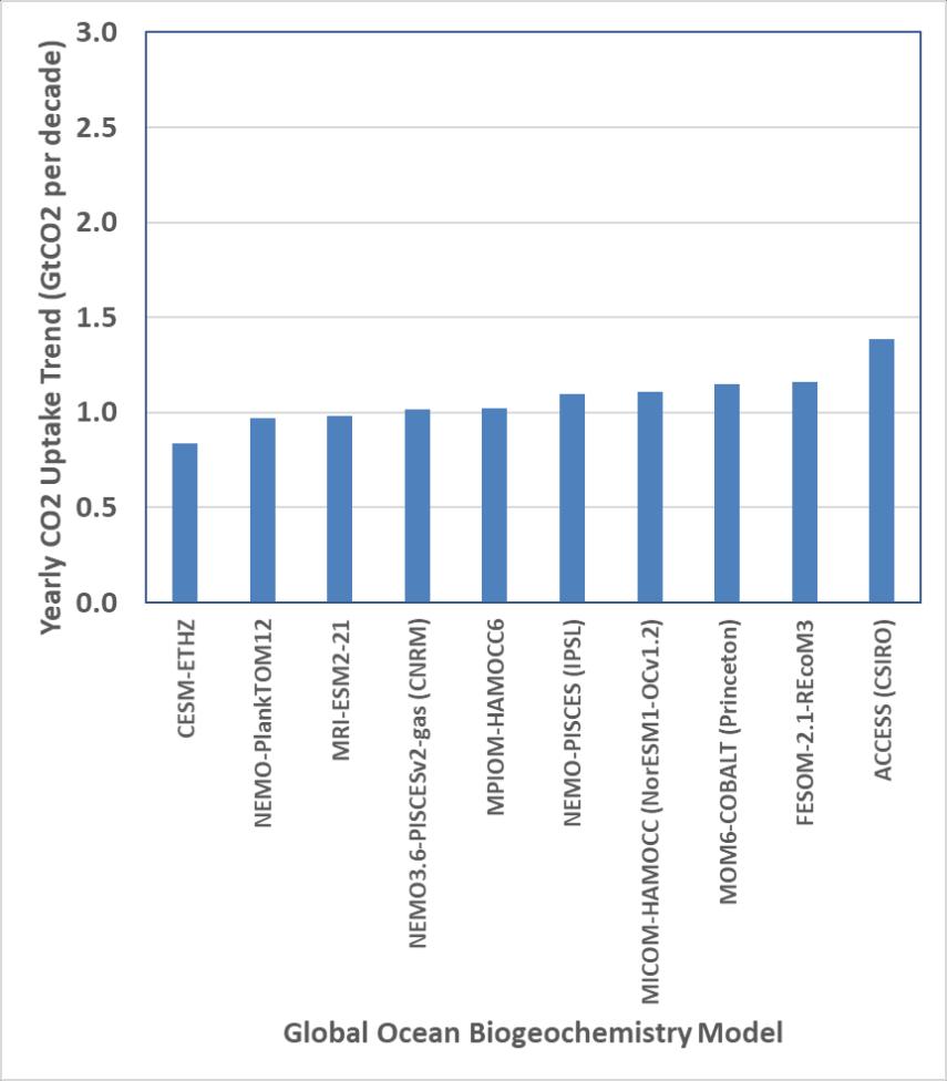
Figure 3.2.4 Trends of annual CO2 uptake (GtCO2 per year per decade) by ocean processes during 1959-2023 simulated by 10 different ocean biogeochemistry models periodically reported by the Global Carbon Project (Friedlingstein, 2024).

3.3 Urbanization influence on temperature trends

Historical temperature data over land has been collected mainly where people live. This raises the problem of how to filter out non-climatic warming signals due to Urban Heat Islands (UHI) and other changes to the land surface. If these are not removed the data might over-attribute observed warming to greenhouse gases. The IPCC acknowledges that raw temperature data are contaminated with UHI effects but claims to have data cleaning procedures that remove them. It is an open question whether those procedures are sufficient.

AR6 downplayed this issue by saying (WGI p. 235) that no recent evidence had emerged to alter the AR5 finding that urbanization causes an upward bias of no more than 10 percent in the global land surface warming trend. AR5 (WGI p. 189) also cited the 10 percent upper bound without citing a source. AR4 (WGI p. 244) cited Jones et al. (1990) and Peterson et al. (1999) as the basis of the claim. Peterson et al. had failed to find any difference in trends between rural and urban samples, although their definition of rural included local populations up to 10,000 persons while the relative influence of urbanization begins well below that (Spencer et al., 2025). Jones et al. compared rural/urban warming in three regions: Eastern Australia, Eastern China and Western Soviet Union. Their definition of ‘‘rural’’ included towns of up to

10,000 in the former Soviet Union and up to 100,000 in China. They found relative warming biases greater than 10 percent in these areas but conjectured that the urbanization effect averaged over the areas they did not examine would bring the global land bias to under 10 percent of the observed warming trend.

Several papers appeared in print prior to the IPCC AR4 that argued that the warming effect of UHIs added a relatively large (30-50%) component to observed warming and was not simulated by climate models (de Laat and Maurellis 2006, McKitrick and Michaels 2007). These findings were based on correlations between locations of maximum warming over land with locations of maximum socioeconomic development. AR4 asserted (p. 244) that these correlations were an artefact of natural atmospheric circulations and were in fact statistically insignificant, and on that basis set the findings aside. Their claim was controversial because it was presented with no supporting evidence. McKitrick (2010) and McKitrick and Nierenberg (2010) showed that taking into account various conjectured alternative explanations for the correlations did not affect their significance. AR5 (p. 189) conceded that AR4 had provided “no explicit evidence” for its assessment and further acknowledged, based on these papers, that there was “significant evidence for such contamination of the record” i.e. a warming bias in the land record. However as already noted, elsewhere in the AR5 report they carried forward AR4 claim that it was less than 10 percent of observed warming. Further they provided no caution about using the land record for climate measurement despite conceding the evidence for UHI contamination. Recently Soon et al. (2023) estimated an urbanization bias in the Northern Hemisphere land record over 1850-2018 sufficient to increase the trend in the blended record from 0.55°C to 0.89°C per century.

Some studies providing evidence against UHI contamination compared warming rates between rural and urban locations (Jones et al. 1990, Peterson et al. 1999, Wickham et al. 2013). It is not known whether such methods would be capable of detecting UHI bias even when present. The influence of UHI warming is logarithmic in population, in other words it is strongest at low population density then levels off as local urbanization expands (Oke 1973, Spencer et al. 2025). Hence failure to find a difference in warming rates between urban and rural stations does not prove the absence of UHI contamination. McKitrick (2013) provided an empirical demonstration in which the rural/urban trends were not significantly different in a data set shown on other grounds to be contaminated with UHI bias.

Parker (2006) examined a sample of urban locations and found no difference in trends between subsets partitioned according to nighttime wind speed, concluding on this basis that urbanization could not be a significant factor. Here again the question is whether such a method would find UHI bias even if present. McKitrick (2013) presented an example in which UHI-contaminated data did not exhibit significant trend differences when stratified according to wind speed.

The challenge in measuring UHI bias is relating local temperature change to a corresponding change in population or urbanization, rather than to a static classification variable such as rural or urban. Spencer et al. (2025) used newly available historical population archives to undertake such an analysis and found evidence of significant UHI bias in U S summertime temperature data.

In summary, while there is clearly warming in the land record, there is also evidence that it is biased upward by patterns of urbanization and that these biases have not been completely removed by the data processing algorithms used to produce climate data sets.

References

Angert, A., S. Biraud, Bonfils, C., Buermann, W. and I. Fung (2004). CO2 seasonality indicates origins of post-Pinatubo sink. Geophysical Research Letters 31. https://doi.org/10.1029/2004GL019760

AR6: Intergovernmental Panel on Climate Change Sixth Assessment Report (2021) Working Group I Contribution. www.ipcc.ch

AR5: Intergovernmental Panel on Climate Change Fifth Assessment Report (2013) Working Group I Contribution. www.ipcc.ch

AR4: Intergovernmental Panel on Climate Change Fourth Assessment Report (2007) Working Group I Contribution. www.ipcc.ch

Burgess, Matthew et al (2021) Environmental Research Letters 16 014016 https://iopscience.iop.org/article/10.1088/1748-9326/abcdd2/meta

Ciais, P., C. Sabine, G. Bala, L. Bopp, V. Brovkin,et al. (2013): Carbon and Other Biogeochemical Cycles. In: Climate Change 2013: The Physical Science Basis. Contribution of Working Group I to the Fifth Assessment Report of the Intergovernmental Panel on Climate Change [Stocker, T.F., D. Qin, G.-K. Plattner, M. Tignor,et al. (eds.)]. Cambridge University Press, Cambridge, United Kingdom and New York, NY, USA

Connolly, Roman, Willie Soon, Michael Connolly et al. (2021) How much has the Sun influenced Northern Hemisphere temperature trends? An ongoing debate Research in Astronomy and Astrophysics 21(6) doi: 10.1088/1674-4527/21/6/131 https://iopscience.iop.org/article/10.1088/16744527/21/6/131

Crisp, David & Dolman, Han (A.J.) & Tanhua, Toste & Mckinley, Galen & Hauck, Judith & Bastos, Ana & Sitch, Stephen & Eggleston, Simon & Aich, Valentin. (2022). How Well Do We Understand the Land‐Ocean‐Atmosphere Carbon Cycle?. Reviews of Geophysics. 60. 10.1029/2021RG000736.

De Laat, A.T.J., and A.N. Maurellis (2006), Evidence for influence of anthropogenic surface processes on lower tropospheric and surface temperature trends, International Journal of Climatology 26:897 913. Friedlingstein, P., and 95 co-authors (2024): Global Carbon Budget 2024, Earth System Science Data 14(4), https://essd.copernicus.org/preprints/essd-2024-519

Hausfather et al. (2019) “Evaluating the Performance of Past Climate Model Projections” Geophysical Research Letters 47(1) https://doi.org/10.1029/2019GL085378

Hausfather, Z. and G. Peters (2020a) “Emissions – the ‘business as usual’ story is misleading” Nature 29 January 2020 https://www.nature.com/articles/d41586-020-00177-3

Hausfather, Z. and G. Peters (2020b) RCP8.5 is a problematic scenario for near-term emissions. Proceedings of the National. Academy of Sciences 117, 27791–27792 (2020)

Jenkins, S., Smith, C., Allen, M. et al. Tonga eruption increases chance of temporary surface temperature anomaly above 1.5°C. Nature Climate Change. 13, 127–129 (2023). https://doi.org/10.1038/s41558022-01568-2

Jones, P. D., P. Y. Groisman, M. Coughlan, N. Plummer, W.-C. Wang, and T. R. Karl (1990), Assessment of urbanization effects in time series of surface air temperature over land, Nature, 347, 169 – 172

Liu, Pengfei et al. (2021) “Improved estimates of preindustrial biomass burning reduce the magnitude of aerosol climate forcing in the Southern Hemisphere” Science Advances 7(22) May 2021 https://doi.org/10.1126/sciadv.abc1379

McKitrick, R.R. and P.J. Michaels (2007), Quantifying the influence of anthropogenic surface processes and inhomogeneities on gridded global climate data, Journal of Geophysical Research, 112, D24S09, doi:10.1029/2007JD008465.

McKitrick, Ross R. (2010) Atmospheric Oscillations Do Not Explain the Temperature-Industrialization Correlation. Statistics Politics and Policy Vol 1. No. 1., July 2010

McKitrick, Ross R. (2013) Encompassing Tests of Socioeconomic Signals in Surface Climate Data Climatic Change doi 10.1007/s10584-013-0793-5. Volume 120, Issue 1-2 http://link.springer.com/article/10.1007%2Fs10584-013-0793-5

McKitrick, Ross R. and Nicolas Nierenberg (2010) Socioeconomic Patterns in Climate Data. Journal of Economic and Social Measurement, 35(3,4) pp. 149-175. DOI 10.3233/JEM-2010-0336

McKitrick, Ross R., Mark Strazicich and Junsoo Lee (2012) “Long-Term Forecasting of Global Carbon Dioxide Emissions: Reducing Uncertainties Using a Per-Capita Approach.” Journal of Forecasting, Vol 32, Issue 5, pp 435-451 DOI: 10.1002/for.2248.

Oke, T.R., 1973: City size and the urban heat island, Atmospheric Environment 7, 769-779

Parker, D.E. (2006) “A Demonstration that Large-Scale Warming is not Urban.” Journal of Climate 19:2882 2895.

Peterson, Thomas C., Kevin P. Gallo, Jay Lawrimore, Timothy W. Owen, Alex Huang, David A. McKittrick (1999) Global rural temperature trends Geophysical Research Letters February 1999 https://doi.org/10.1029/1998GL900322

Pielke Jr., Roger and Ritchie, Justin (2020) “Systemic Misuse of Scenarios in Climate Research and Assessment” Social Sciences Research Network April 2020, available at: https://ssrn.com/abstract=3581777

Pielke Jr, R., Burgess, M. G., & Ritchie, J. (2022). Plausible 2005-2050 emissions scenarios project between 2 and 3 degrees C of warming by 2100. Environmental Research Letters 17 024027 https://iopscience.iop.org/article/10.1088/1748-9326/ac4ebf/pdf

Scaffeta, Nicola, Richard C. Willson, Jae N. Lee and Dong Wu (2019) Modeling Quiet Solar Luminosity Variability from TSI Satellite Measurements and Proxy Models during 1980–2018 Remote Sensing 11(21) 2569 https://doi.org/10.3390/rs11212569

Schoeberl, M.R., Y. Wang, G. Taha, D.J. Zawada, R. Ueyama and A. Dessler, 2024. Evolution of the climate forcing during the two years after the Hunga Tonga-Hunga Ha’apai eruption. Journal of Geophysical Research., 129

Schwalm, C.R., S. Glendon, P. B. Duffy (2020) RCP8.5 tracks cumulative CO2 emissions. Proceedings of the National Academy of Sciences U.S.A. 117, 19656–19657 (2020).

Soon,W.; Connolly, R.; Connolly, M.; Akasofu, S.-I.; Baliunas, S.; et al. (2023) The Detection and Attribution of Northern Hemisphere Land Surface Warming (1850–2018) in Terms of Human and Natural Factors: Challenges of Inadequate Data. Climate 2023, 11, 179. https://doi.org/10.3390/cli11090179

Spencer, Roy W, John R Christy and William D. Braswell (2025) Urban Heat Island Effects in U.S. Summer Surface Temperature Data, 1895–2023 Journal of Applied Meteorology and Climatology April 2025 https://doi.org/10.1175/JAMC-D-23-0199.1

Wickham C, R Rohde , RA Muller, J Wurtele, J Curry, et al. (2013) Influence of Urban Heating on the Global Temperature Land Average using Rural Sites Identified from MODIS Classifications. Geoinformatics and Geostatistics: An Overview 1:2.

Zacharias, Pia (2014) An Independent Review of Existing Total Solar Irradiance Records. Surveys in Geophysics 35 pp. 897 912 https://link.springer.com/article/10.1007/s10712-014-9294-y

PART II: CLIMATE RESPONSE TO CO2 EMISSIONS

4 CLIMATE SENSITIVITY TO CO2 FORCING

Chapter Summary

There is growing recognition that climate models are not fit for the purpose of determining the Equilibrium Climate Sensitivity (ECS) of the climate to increasing CO2. The IPCC has turned to datadriven approaches including historical data and paleoclimate reconstructions, but their reliability is diminished by data inadequacies.

Data-driven ECSestimates tend tobelowerthanclimate model-generated values. The IPCCAR6 upper bound for the likely range of ECS is 4.0°C, lower than the AR5 value of 4.5°C. This lowering of the upper bound seems well justified by paleoclimatic data. The AR6 lower bound for the likely range of ECS is 2.5°C, substantially higher than the AR5 value of 1.5°C. This raising of the lower bound is less justified; evidence since AR6 finds the lower bound of the likely range to be around 1.8°C.

4.1 Introduction

The magnitude of the climate’s response to increasing concentrations of CO2 is central to the scientific debate on anthropogenic climate change, and so also to the public debate on “climate action.” The simplest measure of thatresponse is the rise in the global average surface temperature, quantified by the Equilibrium Climate Sensitivity (ECS). ECS is defined as the amount of warming expected in response to a doubling of CO2 from its pre-industrial concentration of 280 ppm, after all climate components have had time to adjust. Some components, like temperatures in the lower atmosphere (troposphere), adjust rapidly, while others such as the deep ocean and cryosphere might take as long as centuries. A related measure, the Transient Climate Response (TCR), better describes the shorter time scales; it is defined as the amount of warming when the CO2 concentration is doubled by rising one percent annually for 70 years.

The 1979 Charney Report for the U.S. National Academy of Sciences (National Research Council 1979) proposed that the most likely ECS was 3.0 ± 1.5°C. The IPCC repeatedly reaffirmed that range with only minor variations until its most recent AR6. AR5 termed 1.5–4.5°C as the likely range (66 percent probability) and stated that ECS is extremely unlikely (95 percent probability) to be below 1.0°C and very unlikely (90 percent probability) to exceed 6.5°C.

The uncertainty in ECS has remained stubbornly wide, despite many individual studies that claimed to narrow it (Hausfather 2023) Most recently, AR6 narrowed the likely range to 2.5–4.0°C and deemed the very likely range to be 2.0–5.0°C. This narrowing on the low end is disputed, as will be discussed below.

Uncertainties in ECS are highly consequential for policy making. As will be discussed in Chapter 11, economic models use ECS values to project the costs of CO2 emissions. The traditional value (3.0 °C) has typically yielded modest global social costs of CO2 emissions, sufficient to justify some policy actions, but mostly deferred to later in this century. If ECS is very high (above 4.5°C) immediate aggressive emission controls become more imperative, whereas no CO2 emission controls are economically justifiable for ECS below 2.0°C (Dayaratna et al. 2017, 2020). Obtaining a precise estimate is impossible, so policy making needs to account for the uncertainty.

By itself, the equilibrium warming effect of a doubling of atmospheric CO2 is slightly more than 1°C (Soden and Held 2006). Larger values of ECS arise from positive feedbacks that amplify the CO2 warming. Water vapor feedback is positive: a warmer atmosphere might have more water vapor, which itself is a powerful greenhouse gas. Warmer temperatures also result in less snow and sea ice cover, allowing the Earth to absorb more of the sun’s radiation. Some simple estimates of these feedbacks increase the ECS to around 2°C (Sherwood et al., 2020). Larger values of ECS are associated with positive cloud feedbacks.

Climate scientists use multiple lines of evidence to determine the Equilibrium Climate Sensitivity:

• Climate model simulations

• Historical observations

• Paleoclimatic reconstructions

• Process understanding of feedbacks

4.2 Model-based estimates of climate sensitivity

The ECS ranges given in IPCC AR4 and AR5 were obtained primarily by examining the behavior of large-scale climate models, also called General Circulation Models (GCMs). However, the IPCC changed course in its AR6 when it turned to a more direct data-driven methodology. Here we discuss some of the pitfalls of using GCMs to try to determine the Earth’s climate sensitivity.

ECS can be determined from climate model simulations by doubling the concentration of CO2 and allowing several centuries for the warming to equilibrate. To avoid the need for such long simulations, “effective climate sensitivity” is commonly evaluated from a 150-year simulation in response to a sudden quadrupling of CO2

In principle, ECS is an emergent property of GCMs that is, it is not directly parameterized or tuned but rather emerges in the results of the simulation. Otherwise plausible GCMs and parameter selections have been discarded because of perceived conflict with an expected warming rate, or aversion to a model’s climate sensitivity being outsidean acceptedrange (Mauritsen etal. 2012). Thispractice wascommonplace for the models used in AR4; modelers have moved away from this practice with time. However, even in a CMIP6 model, Mauritsen and Roeckner (2020) state the following regarding their Max Planck Institute (MPI) climate model (emphasis added):

“We have documented how we tuned the MPI-ESM1.2 global climate model to match the instrumental record of warming; an endeavor which has clearly been successful. Due to the historical order of events, the choice was to do this practically by targeting an ECS of about 3 K using cloud feedbacks, as opposed to tuning the aerosol forcing.”

In other words, the MPI modelers chose an ECS value of 3°C and then tuned the cloud parameterizations to match their intended result.

As noted, direct warming from CO2 doubling is only about 1°C (Soden and Held 2006); further warming arises from climate feedbacks that are not explicitly resolved by the GCM but rely on parameterizations of physical processes. Higher values of ECS arise primarily from positive cloud feedbacks, whereas the magnitude and even the sign of the feedbacks are very uncertain. Elements of cloud feedback include changes in the latitudinal distributionofclouds,changesinthedistributionofcloudheight (changes in low versus high clouds), changes to the phase of clouds (ice versus liquid), changes in cloud particle size (associated with changes in concentration and/or composition of aerosol particles), changes in the precipitation efficiency of clouds, and even changes in how clouds are distributed over the daily solar cycle(Curryand Webster, 1999).It is difficult for GCMs to simulate any of these processescorrectly owing to their small scale, let alone predict how they will change in the future. Further, cloud processes modulate the magnitudes of the water vapor, lapse rate, and the surface albedo feedbacks.

Figure 4.1 Equilibrium Climate Sensitivities in °C of 37 climate models from the CMIP6 ensemble. Identifiers for the various models appear along the horizontal axis. From (Scafetta, 2021)

The spread of ECS values from the CMIP5 ensemble of climate models used in AR5 was 2.0–4.7°C; that range increased for the CMIP6 models used in AR6 to between 1.8 and 5.7°C (Chen et al., 2021, Scaffeta 2021, see Figure 4.1). Far from resolving the model-based climate sensitivity the range appears to be growing. The main cause of the overall upward shift in ECS in CMIP6 relative to CMIP5 is a larger positive cloud feedback, driven by changes to the cloud parameterizations in many CMIP6 models (Zelinka et al., 2020)

Because of concerns about model tuning and the high sensitivity to cloud parameterizations, AR6 (2021) did not rely on climate model simulations in their assessment of climate sensitivity, relying insteadon data-driven methods.

4.3

Data-driven estimates of climate sensitivity

Climate sensitivity can also be estimated from instrumental records of surface temperatures and ocean heat content, combined with estimates of how climate forcings (e.g., greenhouse gases, solar, volcanoes, aerosols) have changed in the past (Otto et al., 2013). Using this information, a simple empirical Energy BalanceModelcanbeemployed.Itrequiresestimatingafeedbackparameterwhoseuncertaintiesarehighly amplified in the resulting ECS (Roe and Baker, 2007).

The accuracy of the data-driven methods depends on the quality of the input data. Assumptions are needed about ocean heat storage, and good data is only available for recent decades. The greatest source of uncertainty is the amount and composition of aerosol particles and their interactions with cloud radiative

properties (the so-called aerosol indirect effect; see Figures 3.1.1, 3.1.2). Climate models exhibit warming in response to GHGs but cooling in response to aerosols (Schwartz et al., 2007). Observed 20th century warming can be shown to be consistent either with low ECS and low aerosolcooling, or high ECS and high aerosol cooling. Since fossil fuel use adds both GHGs and aerosols to the atmosphere, both effects need to be estimated to isolate the warming effect of CO2

Paleoclimate proxies are also used to evaluate the sensitivity of past climates by comparing paleoclimate changes in the Earth’s temperatures to estimates of changes in forcings. The two most informative periods are the lastglacial maximum (around20,000 years ago), which was about 3–7°Ccolder than today, and a mid-Pliocene period (roughly three million years ago), which was 1–3°C warmer than today. The limits on cooling during the last glacial maximum give the best single evidence that high values of climate sensitivity are unlikely. However, paleoclimate estimates are associated with very large uncertainties in the estimated temperatures and forcings. Further, estimates of climate sensitivity based on past climate states might not be applicable to the current state of the climate system.

A recurring theme in the climate literature is that ECS estimates based on historical data are smaller than ECS estimates inferred from climate models (Sherwood and Forest 2024). About 15 estimates based on historical data appeared in the peer-reviewed literature between 2012 and 2024 yielding ECS best estimates between 1.0°C and 2.5°C, although critics have questioned some of the methods and the data quality. For AR6, the IPCC placed primary weight on the results of Sherwood et al. (2020) that combined historical data and paleoclimate proxies with the process-based approach and yielded a best estimate of 3.1°Cwith a likely range of2.6-3.9°C. Lewis(2022)raiseda number ofconcerns about thisresult, including methodological errors, outdated input values, and use of subjective Bayesian priors in the analysis. Lewis’ analysis found that climate sensitivity is estimated to be much lower and better constrained than in the Sherwood et al. analysis – median 2.2°C (1.8–2.7°C in the 17–83 percent likely range, and 1.6–3.2°C in the 5–95 percent very likely range). The IPCC AR6 estimated only a 5 percent probability that ECS was below 2.3°C, whereas Lewis estimated it to be over 50 percent. The most recent publications on the debate between Sherwood et al. and Lewis further defend their respective positions: Sherwood and Foster (2024) and Lewis (2025).

AnargumentemphasizedinAR6isthatdata-drivenECSestimatesmightunderstatethefuturewarming response to GHGs because of a so-called “pattern effect” (Forster et al., 2021). The tropical Pacific is believed to strongly influence the overall efficiency with which the Earth radiates heat to space, but some regions remove heat more efficiently than others. If the west-to-east temperature gradient in the tropical Pacific is weakened in a warming climate, warming would concentrate where heat is less efficiently removed, raising ECS.

Most climate models simulate that rising GHGs will weaken the west-east temperature gradient, which led the IPCC in AR6 to conclude that data-driven ECS estimates understated the future ECS value. However, Seager et al. (2019) pointed out that, contrary to models, the west-east temperature gradient has been strengthening over time. They further argued that the mechanism predicting otherwise in climate models was based on a faulty characterization of oceanic dynamics and there is no reason to expect the gradient to weaken. A similar argument was recently made by Lee et al. (2024), who concluded that “the trajectory of the observed trend reflects the response to increasing GHG loading in the atmosphere”; in otherwords,GHGwarmingshould leadtoafuturestrengtheningratherthanaweakeningofthetemperature gradient. Increased efficiency of atmospheric cooling implies, if anything, that the future ECS in a warming climate might be lower than current estimates.

4.4

Transient Climate Response

The Transient Climate Response (TCR) provides a more useful observational constraint on climate sensitivity. TCR is the global temperature increase that results when CO2 is increased at an annual rate of 1 percent over a period of 70 years (i.e., doubled gradually). Relative to the ECS, observationally determined values of TCR avoid the problems of uncertainties in ocean heat uptake and the fuzzy boundary in defining equilibrium arising from a range of timescales for the longer-term feedback processes (e.g., ice sheets). TCR is better constrained by historical warming, than ECS. AR6 judged the very likely range of TCR to be 1.2–2.4°C. In contrast to ECS, the upper bound of TCR is more tightly constrained. For comparison, theTCRvaluesdetermined byLewis(2023)are 1.25to 2.0°C, showing much betteragreement with AR6 values than was seen in a comparison of the ECS values.

References

Carbon Brief. (2020, July 22). Explainer: How scientists estimate climate sensitivity. https://www.carbonbrief.org/explainer-how-scientists-estimate-climate-sensitivity

Carbon Brief. (2020, July 22). Guest post: Why low-end ‘climate sensitivity’ can now be ruled out. https://www.carbonbrief.org/guest-post-why-low-end-climate-sensitivity-can-now-be-ruled-out Carbon Brief. (2021, August 9). In-depth Q&A: The IPCC’s sixth assessment report on climate science. https://www.carbonbrief.org/in-depth-qa-the-ipccs-sixth-assessment-report-on-climate-science Chen, D., et al. (2021). Framing, context, and methods. In V. Masson-Delmotte et al. (Eds.), Climate change 2021: The physical science basis. Contribution of Working Group I to the Sixth Assessment Report of the Intergovernmental Panel on Climate Change. Cambridge University Press. Curry, J. A., & Webster, P. J. (1999). Thermodynamic feedbacks in the climate system. In Thermodynamics of atmospheres and oceans (pp. 351–385). Academic Press.

Dayaratna,Kevin, Ross McKitrickandDavid Kreutzer(2017) Empirically-Constrained Climate Sensitivity and the Social Cost of Carbon. Climate Change Economics April 2017 DOI: http://dx.doi.org/10.1142/S2010007817500063

Dayaratna, Kevin, Ross McKitrick and Patrick J. Michaels (2020) Climate Sensitivity, Agricultural Productivity and the Social Cost of Carbon in FUND. Environmental Economics and Policy Studies https://doi.org/10.1007/s10018-020-00263-w

Forster, P., et al. (2021). The Earth's energy budget, climate feedbacks, and climate sensitivity. In V. Masson-Delmotte et al. (Eds.), Climate change 2021: The physical science basis. Contribution of Working Group I to the Sixth Assessment Report of the Intergovernmental Panel on Climate Change. Cambridge University Press.

Hausfather, Z. (2020, July 22). Explainer: How scientists estimate climate sensitivity. Carbon Brief. https://www.carbonbrief.org/explainer-how-scientists-estimate-climate-sensitivity

Lan, X., Tans, P., & Thoning, K. W. (2025). Trends in globally-averaged CO₂ determined from NOAA Global Monitoring Laboratory measurements. NOAA Global Monitoring Laboratory. https://doi.org/10.15138/9N0H-ZH07

Lee, S., Byrne, M. P., Loikith, P. C., & O’Dell, C. W. (2024). Zonal contrasts of the tropical Pacific climate predicted by a global constraint. Climate Dynamics, 62(1–2), 229–246. https://doi.org/10.1007/s00382-023-06741-7

Lewis, N. (2023). Objectively combining climate sensitivity evidence. Climate Dynamics, 61(9–10), 3155–3163. https://doi.org/10.1007/s00382-022-06398-8

Lewis, N. (2025). Comment on “Can uncertainty in climate sensitivity be narrowed further?” by Sherwood and Forest (2024). EGUsphere [preprint]. https://doi.org/10.5194/egusphere-2025-1179

Thorsten Mauritsen et al., (2012) “Tuning the Climate of a Global Model,” Journal of Advances in Modeling Earth Systems 4, no. 3 https://doi. org/10.1029/2012ms000154

Mauritsen, T., & Roeckner, E. (2020). Tuning the MPI-ESM1.2 global climate model to improve the match with instrumental record warming by lowering its climate sensitivity. Journal of Advances in Modeling Earth Systems, 12, e2019MS002037. https://doi.org/10.1029/2019MS002037

Otto, A., Otto, F. E. L., Boucher, O., Church, J., Hegerl, G., Forster, P. M., Gregory, J. M., & Johnson, G. C. (2013). Energy budget constraints on climate response. Nature Geoscience, 6(6), 415–416. https://doi.org/10.1038/ngeo1836

Pachauri, R. K., & Meyer, L. (Eds.). (2015). Climate change 2014: Synthesis report. Intergovernmental Panel on Climate Change.

Roe, G. and M. Baker (2007). Why is climate sensitivity so unpredictable? Science 318, 629-632. https://doi.org/10.1126/science.1144735

Scafetta, N. (2021). Testing the CMIP6 GCM simulations versus surface temperature records from 1980–1990 to 2011–2021: High ECS is not supported. Climate, 9(11), 161. https://doi.org/10.3390/cli9110161

Schwartz, S. E., R. J. Charlson, H. Rodhe (2007). Quantifying climate change Too rosy a picture? Nature Climate Change 1, 23–24, https://doi.org/10.1038/climate.2007.22

Seager, R., Cane, M., Ting, M., Naik, N., Clement, A., DiNezio, P., & Lee, D. E. (2019). Strengthening tropical Pacific zonal sea surface temperature gradient consistent with rising greenhouse gases. Nature Climate Change, 9(7), 517–522. https://doi.org/10.1038/s41558-019-0505-x

Sherwood, S. C., & Forest, C. E. (2024). Opinion: Can uncertainty in climate sensitivity be narrowed further? Atmospheric Chemistry and Physics, 24(5), 2679–2686. https://doi.org/10.5194/acp-24-26792024

Sherwood, S. C., Bony, S., Boucher, O., Bretherton, C. S., Forster, P. M., Gregory, J. M., & Stevens, B. (2020). An assessment of Earth's climate sensitivity using multiple lines of evidence. Reviews of Geophysics, 58(4). https://doi.org/10.1029/2019rg000678

Soden, B. J., and I.M. Held (2006). An assessment of climate feedbacks in coupled ocean–atmosphere models. Journal of Climate, 19(14), 3354–3360. https://doi.org/10.1175/jcli3799.1

Zelinka, M. D., Myers, T. A., McCoy, D. T., Po-Chedley, S., Caldwell, P. M., Ceppi, P., Klein, S. A., & Taylor, K. E. (2020). Causes of higher climate sensitivity in CMIP6 models. Geophysical Research Letters, 47, e2019GL085782. https://doi.org/10.1029/2019GL085782

5 DISCREPANCIES BETWEEN MODELS AND INSTRUMENTAL

OBSERVATIONS

Chapter summary

Climate models show warming biases in many aspects of their reproduction of the past several decades. In response to estimated changes in forcing they produce too much warming at the surface (except in the models with lowest ECS), too much warming in the lower-and mid-troposphere and too much amplification of warming aloft.

Climate models also produce too much recent stratospheric cooling, invalid hemispheric albedos, too much snow loss, and too much warming in the Corn Belt. The IPCC has acknowledged some of these issues but not all.

5.1 Introduction

Climate models are the primary tool used to project future climate changes in response to increasing atmospheric levels of anthropogenic greenhouse gases. To assess the fitness of climate models for this purpose, it is reasonable to ask how well they reproduce the current climate and its variations over the past century. The box “Climate modeling” gives some detail on how climate models work.

Of great concern is the fact that, after several decades of the climate modeling enterprise involving approximately three dozen models operated by research centers around the world, the range of future warming they produce in response to a hypothetical doubling of atmospheric CO2 extends over a factor of three, as we discussed in the previous chapter. This range of disagreement among models has not decreased for decades.

Problems with climate models are not just in their disagreement over the future, but also in their ability to replicate the recent past. Here we review some of the most important metrics of climate model accuracy: ability to reproduce historical surface, tropospheric and stratospheric temperature trends; ability to reproduce the vertical warming profile; and ability to reproduce other climate features such as snowfall. In all cases a persistent finding is that models on average err on the side of too much warming in response to estimated historical forcings.

BOX: Climate modeling

All but the simplest climate models represent Earth's land surface using a grid of squares some 100 km wide. To simulate the atmosphere, typically 30 or more grid boxes are stacked above these squares. The ocean is modeled using a similar but finer grid, resulting in tens of millions of grid boxes for the atmosphere and oceans.

The computer models, based on physical laws, calculate how air, water, and energy move between grid boxes over time. The time step can be as small as 10 minutes, and repeating this process millions of times allows the simulation of climate over centuries. Running these models, even on the most powerful supercomputers, can take months. Comparing simulation results with historical climate data helps assess the accuracy of a model, while projections into the future estimate climate changes under assumed human and natural influences.

Despite sounding straightforward, climate modeling is highly complex. Many critical processes occur at scales smaller than the grid size. For instance, the flows of sunlight and heat in the atmosphere depend strongly on cloud cover. Since tracking individual clouds is impractical, researchers must make “subgrid” assumptions about the distribution of clouds in each grid box. Snow and ice cover, which affects how much sunlight is reflected or absorbed by the surface, is another subgrid factor.

Each subgrid assumption requires numerical parameters, which must be carefully set. Modelers initially estimate these parameters based on physics and observed climate patterns, then run the model. Because early results often diverge significantly from real-world observations, they “tune” these parameters to better match observed climate features. Different modeling teams use distinct assumptions and tuning strategies, leading to varied outcomes. Tuning is a necessary but delicate aspect of climate modeling, as it is for any complex system. Poor tuning can result in inaccurate simulations, while excessive tuning risks artificially steering results toward predetermined conclusions.

The spread of model representations of the current climate is very wide. One of the most basic indicators Earth’s average surface temperature varies by about 3ºC across CMIP6 models prior to 1880 (Figure 5.1), narrows slightly until 2040 then diverges to over 4 °C. For comparison 20th century warming was only about 1.0°C. This variation suggests substantial differences among models’ physical processes

Beyond the models’ ability to reproduce features of today’s climate, the critical issue for society is how well they predict responses to subtle human influences, such as greenhouse gas emissions, aerosol cooling, and landuse changes. The most crucial aspect that models must capture correctly is “feedbacks.” These occur when climate changes either amplify or suppress further warming. In general, the modeled net effect of all feedbacks doubles or triples the direct warming impact of CO₂.

Figure 5.1 CMIP6 Average surface temperature range across 33 models and standard deviation using SSP5-85 scenario Data from KNMI Climate Explorer website at https://climexp.knmi.nl/start.cgi

5.2 Surface warming

A straightforward test of a climate model’s validity is its ability to reproduce historical warming in response to known past changes in climate drivers such as greenhouse gases. Figure 5.2 is reproduced from Scaffeta (2023), that groups the latest-generation (CMIP6) climate models into low ECS (1.5 to 3.0 degrees C), medium ECS (3.0 to 4.5 degrees C) and high ECS (4.5 to 6.0 degrees C), and compares their post-1980 globalaveragetemperaturesimulationrangestothoseofthreesurfacetemperaturerecordsandonesatellitebased lower troposphere temperature data product.

The leftmost column shows that the low-ECS models track the post-1980 historical warming record reasonably well, but the middle and right columns show that the medium- and high-ECS models conspicuously over-predict the warming.

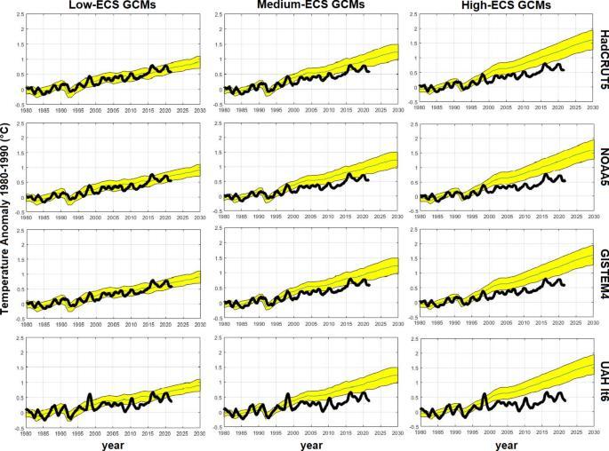
Figure 5.2: Model-Observational comparisons for Earth’s surface warming. The columns correspond to model groups showing low-ECS (13 models) medium-ECS (11 models) and high-ECS (14 models), while the rows correspond to widely-used observed temperature records, the first three showing surface averages and the fourth showing the lower troposphere average. In each panel the yellow area denotes the mean and range (± one standard deviation) of climate model simulations for that group. The thick black line shows the observed annual average temperature in the indicated record

Source: Scafetta (2023) Fig.2.

Spencer (2024) has also provided a useful summary of the Model-Observation mismatch by comparing trends in surface temperature data products with those in individual climate models, as summarized in Figure 5.3; most climate models show substantially more warming than the observations since 1979

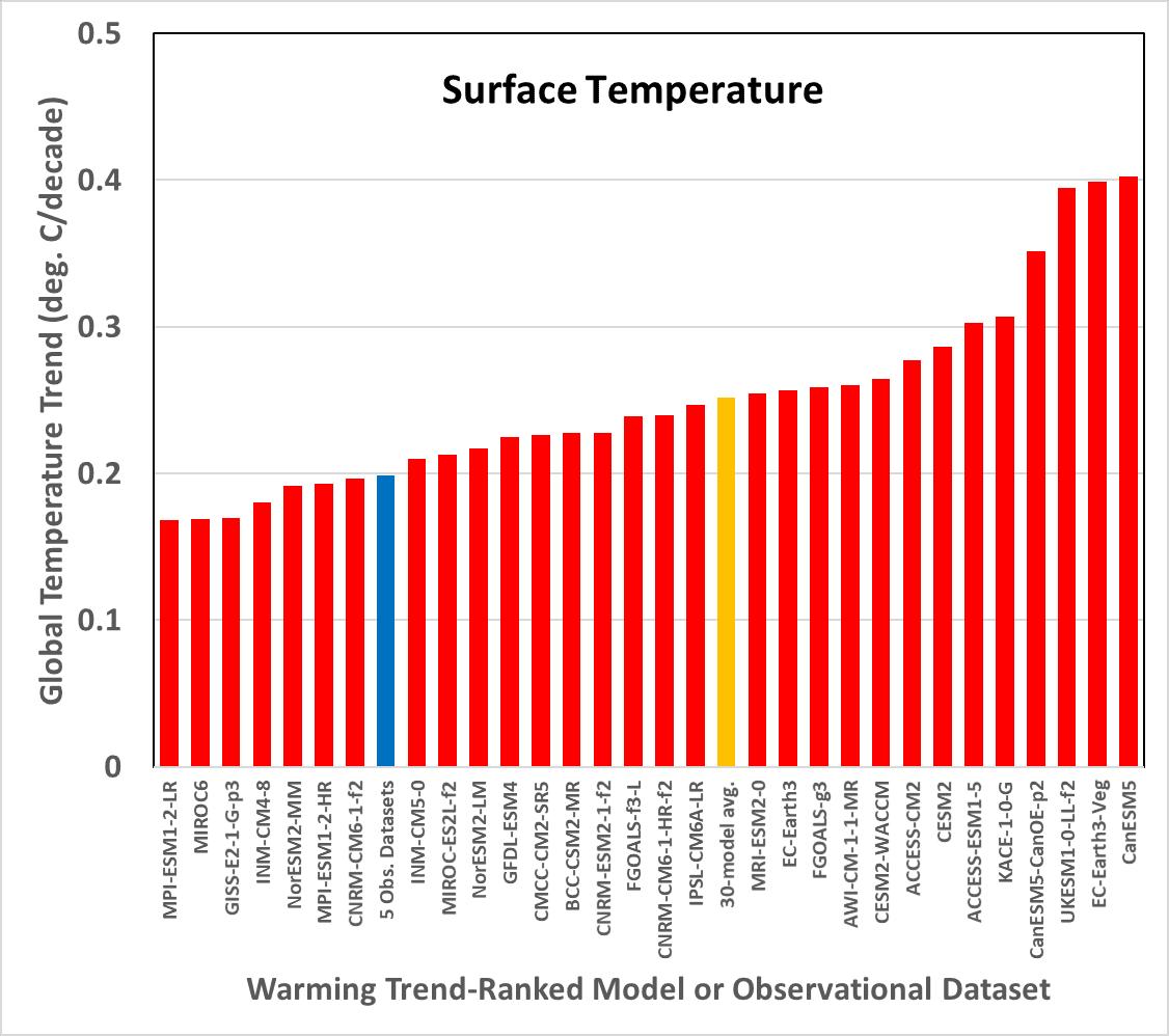
Figure 5.3 Global surfaceairtemperaturetrends (°C/decade), 1979-2024,from various CMIP6 climate models (red, 30-model average in orange); and the average of three thermometer datasets (HadCRUT5, NOAA Global Temp, and Berkeley 1 deg.) and two reanalysis datasets (ERA5 and NCEP/NCAR R1) in blue. Data source: https://climexp.knmi.nl/start.cgi.

5.3 Tropospheric warming

It has long been known that climate models on average overstate warming in the tropical troposphere. Thisregion isan important testofclimate models since this is where thesignal ofanthropogenic greenhouse warming emergesfirstandmoststrongly. Biases in tropospheric trends indicate modelflaws in heat transfer processes that carry over to surface warming biases.

The discrepancy was flagged as a serious inconsistency in the first U.S. Climate Change Science Program report (Karl et al. 2006) and has been mentioned in every IPCC report since, but the discrepancy has gotten worse over time, and the bias is now global. McKitrick and Christy (2020) compared tropospheric warming trends in CMIP6 climate models to observed trends from satellites, weather balloons and reanalysis systems Every model overpredicted the average observed warming trend over 1979-2014 in both Lower- and Mid-Troposphere layers, both globally and in the tropics. In most individual models the bias was statistically significant and on average across models it was highly significant.

Figure 5.4 presents the comparisons with data updated to 2024 (McKitrick and Christy 2025). The recent warm years moved the observed trend up slightly and widened the trend confidence intervals but the overall pattern remains the same: model bias is towards too much warming, in most cases the difference is statistically significant and on average the bias is statistically highly significant. McKitrick and Christy (2020) also showed that the bias is larger in high-ECS models, but even the models with lower average ECS predict too much warming. If future climate models were to realistically represent global tropospheric warming, they would likely be less sensitive than even the low-ECS members of the CMIP6 ensemble.

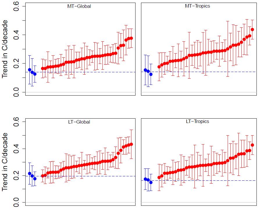
Figure 5.4: Observed versus CMIP6 modeled warming trends (°C/decade 1979-2024) in the global and tropical lower (LT) and mid-troposphere (MT) using the methodology of McKitrick and Christy (2020) on data updated from 2014 to 2024 Blue dots: warming trends with 95 percent confidence intervals for 3 data products (radiosondes, reanalysis, and satellites). Blue dashed line: warming trend average for 3 observed series. Red dots: modeled warming trends with 95 percent confidence intervals in 35 models arranged lowest to highest.

As mentioned previously, the IPCC has long acknowledged the model-observation mismatch. For example, AR6 pp. 443-444 offers this on the tropical troposphere (it does not address the global comparison):

Several studies since AR5 have continued to demonstrate an inconsistency between simulated and observed temperature trends in the tropical troposphere, with models simulating more warming than observations (Mitchell et al., 2013, 2020; Santer et al., 2017a, b;McKitrick and Christy, 2018; Po-Chedley et al., 2021)… Over the 1979–2014 period, models are more consistent with observations in the lower troposphere, and least consistent in the upper troposphere around 200 hPa, where biases exceed 0.1°C per decade. Several studies using CMIP6 models suggest that differences in climate sensitivity may be an important factor contributing to the discrepancy betweenthe simulatedandobserved tropospherictemperature trends (McKitrickand Christy, 2020; Po-Chedley et al., 2021), though it is difficult to deconvolve the influence of climate sensitivity, changes in aerosol forcing and internal variability in contributing to tropospheric warming biases (Po-Chedley et al., 2021). Another study found that the absence of a hypothesized negative tropical cloud feedback could explain half of the upper troposphere warming bias in one model (Mauritsen and Stevens, 2015).

… In summary, studies continue to find that CMIP5 and CMIP6 model simulations warm more than observations in the tropical mid- and upper-troposphere over the 1979–2014 period (Mitchell et al., 2013, 2020; Santer et al., 2017a, b; Suárez-Gutiérrez et al., 2017; McKitrick and Christy, 2018), and that overestimated surface warming is partially responsible (Mitchell et al., 2013; PoChedley et al., 2021). …. Hence, we assess with medium confidence that CMIP5 and CMIP6 models continue to overestimate observed warming in the upper tropical troposphere over the 1979–2014 period by at least 0.1°C per decade,

Notably, despite the accumulation of evidence of excess model warming the IPCC assigns only medium confidence to the existence of a warming bias.

5.4 Vertical temperature profile mismatch

Another important model-observational discrepancy is the excess amplification with altitude found in climate models. The comparison was in AR5 Chapter 10, although only in the online supplement (Figure 10.SM.1) and only in a figure whose formatting obscuredthe point. Figure 10.SM.1 is not referenced in the main IPCC report nor in any summary so readers would not have been aware of it Although not apparent at first glance, it shows that the 1979-2010 warming in the lower troposphere is so small as to be consistent with no GHG forcing at all and is inconsistent with the model runs that do have GHG forcing. In Figure 5.6 we adapt IPCC AR5 Figure 10.SM.1 to draw out this critical point.

Figure 5.5: Vertical warming pattern for tropics (20S to 20N). Horizontal axis: °C/decade. Source: Annotated version of IPCC AR5 Figure 10.SM.1

Figure 5.5 compares modeland observational temperature trends by altitude between 20S and 20N (the tropics). In this region where the models say the warming should be strongest, the observations (shown here in white) lie within the blue “No CO2” band and entirely outside the “with CO2” red envelope. This means that in the entire tropical atmospheric column from the surface to the base of the stratosphere, observed warming trends are so small as to be consistent with the output of models that have no anthropogenic CO2, and inconsistent with the entire envelope of warming trends generated by models forced with increased CO2.

A similar comparison is shown in Christy and McNider (2017), an updated version of which (covering 1979-2024) is reproduced as Figure 5.6. Modeled temperature trends exceed observations from the surface through the top of the troposphere, with observed trends below the entire model range at most pressure levels. Also shown in Figure 5.6 is the tropical tropospheric temperature (TTT) average from three satellite data products (NOAA, UAH and RSS) compared to the same layer average from climate models for 19792024. Again, the observed trends lie below the entire model range.

The wide range of choices made by modelers to characterize the physical processes in the models (see Box: Climate Modeling in Section 5.1above) is seenby the large spread oftrendsin themiddle troposphere, ±40 percent about the median (Figure 5.6). This vividly illustrates the uncertainties in attempts to model (parameterize) a complex system involving turbulence, moist thermodynamics, and energy fluxes over the full range of the tropical atmosphere’s time and space scales.

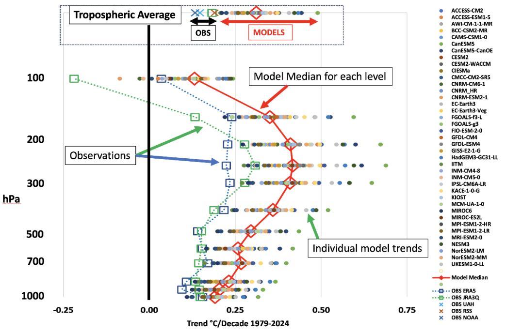
Figure 5.6: Modeled versus observed warming, tropical troposphere. Source: updated from Christy and McNider (2017) including data through 2024 and CMIP6 model outputs Red line: model average. Green and blue lines: observational series (reanalysis).

This discrepancy has been the source of much controversy, with some arguing that even if there is very little observed warming aloft in the tropics, a “hotspot” still exists in the sense that the warming aloft is greater than at the surface (Santer et al. 2008). But there is good evidence that models also exaggerate the amplification rate. Klotzbach et al. (2009), showed that models project greater amplification with altitude than is observed. This result was subsequently confirmed by detailed time series analysis (Vogelsang and Nawaz 2016) which found that the model-observational difference is statistically significant.

The atmosphere’s temperature profile is a case where models are not merely uncertain but also show a common warming bias relative to observations. This suggests that they misrepresent certain fundamental feedback processes.

The IPCC AR6 did not assess this issue.

5.5 Stratospheric cooling

An important element of the expected general “fingerprint” of anthropogenic climate change is simultaneous warming of the troposphere and cooling of the stratosphere. The latter feature is also influenced by ozone depletion and recovery. AR6 acknowledged that cooling had been observed but only until the year 2000. The stratosphere has shown some warming since, contrary to model projections

AR6 WG1 Ch 2 pp. 327-9 states:

Temperatures averaged through the full lower stratosphere (roughly 10–25 km) have decreased over 1980–2019 in alldata products, with the bulk of the decrease prior to 2000. The decrease holds even if the influence of the El Chichon (1982) and Pinatubo (1991) volcanic eruptions on the trend, found by Steiner et al. (2020a) to have increased the 1979–2018 cooling trend by 0.06°C per decade, is removed. Most datasets show no significant or only marginally significant trends over 2000–2019, and the results of Philipona et al. (2018) show weak increases over 2000–2015 in the very lowermost stratosphere sampled by radiosondes….

It is virtually certain that the lower stratosphere has cooled since the mid-20th century. However, most datasets show that lower stratospheric temperatures have stabilized since the mid-1990s with no significant change over the last 20 years. It is likely that middle and upper stratospheric temperatures have decreased since 1980, but there is low confidence in the magnitude.

The cited source, Philipona et al. (2018), in an article entitled “Radiosondes Show That After Decades of Cooling, the Lower Stratosphere Is Now Warming”, stated:

In response to continued greenhouse gas increases and stratospheric ozone depletion, climate models projectcontinued tropospheric warming andstratosphericcooling over thecoming decades. Global average satellite observations of lower stratospheric temperatures exhibit no significant trends since the turn of the century. In contrast, an analysis of vertically resolved radiosonde measurements from 60 stations shows an increase of lower stratospheric temperature since the turn of the century at altitudes between 15 and 30 km and over most continents. Trend estimates are somewhat sensitive to homogeneity assessment choices, but all investigated radiosonde data sets suggest a change from late twentieth century cooling to early 21st century warming in the lower stratosphere.

Santer et al. (2023) use updated data to show that a cooling trend has not re-emerged in the lower stratosphere.

A combination of tropospheric warming and stratospheric cooling is a commonly cited “fingerprint” of anthropogenic climate change. Stratospheric warming since 2000 coincides with continued surface and tropospheric warming, a pattern that is not found in climate model simulations and is not apparently consistent with the anthropogenic fingerprint.

5.6

Snow cover mismatch

Data compiled by the Rutgers University Snow Lab show that Northern Hemisphere winter snow cover is not decreasing (Figure 5.7); if anything, it shows an increasing trend.

Figure 5.7: Northern Hemisphere Winter Snow extent. Source: https://climate.rutgers.edu/snowcover/chart_seasonal.php?ui_set=nhland&ui_season=1 (accessed May 27, 2025)

Yet models project declining Northern Hemisphere snow cover in a warming climate, as described by Connolly et al. (2019).

The climate models were found to poorly explain the observed trends [in Northern Hemisphere snow cover]. While the models suggest snow cover should have steadily decreased for all four seasons, only spring and summer exhibited a long-term decrease, and the pattern of the observed decreases for these seasons was quite different from the modelled predictions. Moreover, the observed trends for autumn and winter suggest a long-term increase, although these trends were not statistically significant.

AR6 largely confines its discussion of changing Northern Hemisphere snow cover extent (SCE) to the Spring season, for which models and observations agree on a downward trend. Regarding Winter changes it remarks as follows (AR6 WGI Ch. 2 p. 344):

Assessment of SCE trends in the NH since 1978 indicates that for the October to February period there is substantial uncertainty in trends with the sign dependent on the observational product. Analysis using the NOAA Climate Data Record shows an increase in October to February SCE (Hernández-Henríquez et al., 2015; Kunkel et al., 2016) while analyses based on satellite borne optical sensors (Hori et al., 2017) or multi-observation products (Mudryk et al., 2020) show a negative trend for all seasons.

AR6 WGI Chapter 9 (p. 1284) points out that the NOAA Climate Data Record showing increased fall and winter SCE is inconsistent with land-based observations and model-based data sets. It notes that using optical satellite imagery to infer SCE in winter is challenging due to cloud cover and decreased solar illumination in winter months. Focusing on the Pacific Coast states (CA, OR and WA) cold season mountain snowfall that melts in spring and summer provides a substantial portion of warm season water resources. A comprehensive reconstruction of snowfall for the main source regions (Cascades and Sierra Nevada Mountains) indicates no significant trends in annual totals since the late 19th century (Christy 2022).

In summary, the up-to-date Rutgers SCE database indicates a mismatch between models and observations. Further work to reconcile conflicting trends in observational data sets is required.

5.7 Hemispheric symmetry of the planetary albedo

The planetary albedo is the fraction of incoming solar radiation reflected by the Earth back to space. It is an important element of the radiative energy balance and influences whether the planet will warm or cool over time. The planetary albedo is typically estimated at around 0.30; variations on the scale of 0.01 correspond to changes in solar forcing of about 3 W/m2, an amount larger than current anthropogenic forcing. It has long been noted that models disagree with each other and with observations on the value of the global planetary albedo (Stephens et al. 2015).

An intriguing property of the Earth’s albedo is that, on average, the Northern Hemisphere (NH) and Southern Hemisphere (SH) have had nearly the same albedo, at least throughout the fifty-year satellite record (Stephens et al., 2015). This symmetry is surprising, because the SH has much more ocean than land. Since ocean is less reflective than land, the NH should have higher albedo. Clouds (which are highly reflective) are more common in the NH and so compensate the surface albedo imbalances of the two hemispheres. Datseris and Stephens (2021) show that this cloud compensation comes from the extratropical storm tracks of the SH, which are cloudier than those of the NH. While the mechanism for this hemispheric symmetry is unclear, it likely operates on large temporal and spatial scales.

The hemispheric symmetry of the albedo is a simple gross metric for climate models. Rugenstein and Hakuba (2023) defined that metric as the difference between the NH and SH annual mean albedos, expressed as Wm 2 of the reflected sunlight, and compiled it for the CMIP6 climate models, as shown in Figure 5.8. Most of the CMIP6 models do not reproduce the small observed asymmetry (about 0.1 Wm-2) and even disagree as to which hemisphere is more reflective. Moreover, the magnitude of the asymmetry ranges up to 5 Wm-2 in some models, twice as large as the current anthropogenic forcing (about 2.7 Wm-2).

The significance of unphysical albedo asymmetries in the climate models is not yet fully known. However, other model studies suggest that interhemispheric changes in albedo can alter poleward heat fluxes, meridional temperature gradients, storminess, and differences in hemispheric ocean heat storage. The discrepancy between models and observations further raises issues regarding cloud feedback processes and so more generally diminishes confidence in model projections of the future climate.

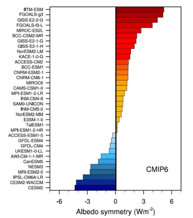
Figure 5.8. Differences in 20-year average reflectivity (albedo) between the Northern and Southern Hemispheres for CMIP6 models used in the most recent IPCC assessment (colored bars). The very small observed difference is indicated by the vertical black line. From Rugenstein and Hakuba (2023).

5.8 U.S. Corn Belt

One of the largest discrepancies between models and observations is in the U.S. Corn Belt, a region of particular importance to global food production. Figure 5.9 shows the warming trends for summertime (June, July, August) for the 12-state Corn Belt (IN, IA, IL, ND, SD, MO, MN, WI, MI, OH, KS, NE) during 1973-2022. All 36 climate models (red) warm far too rapidly compared to observations (blue).

Figure 5.9: Modeled versus observed warming trends in the U.S. Corn Belt, 1973-2022.

As discussed in Chapter 9, the anticipated negative effects of increasing temperatures on U.S. corn yields have not materialized, in contrast to widely publicized studies proclaiming that theoretical future impacts are already being experienced (e.g., Seager et al., 2018).

The IPCC acknowledges limitations in the accuracy of regional climate model outputs. This example shows that users need to assess model projections carefully on a case-by-case basis since local biases might be sufficiently large that the models are simply not fit for purpose. As has recently been noted by two leaders of the modeling community (emphasis added)

… for many key applications that require regional climate model output or for assessing largescale changes from small scale processes, we believe that the current generation of models is not fit for purpose (Palmer and Stevens 2019)

To summarize:

• Climatemodelsshow warmingbiasesinmanyaspectsoftheirreproductionofthepastfewdecades.

• They produce too much warming at the surface (except in the models with lowest ECS), too much warming in the lower-and mid-troposphere and too much amplification of warming aloft

• They also produce too much stratospheric cooling, too much snow loss, and too much warming in the U S Corn Belt.

• The hemispheric albedo difference in individual climate models ranges widely in sign and magnitude compared to observations. The range in W/m2 is three times larger than the direct anthropogenic forcing of CO2

• The IPCC has acknowledged some of these issues but not others.

References

Christy, J. R., R. T. McNider (2017). Satellite bulk tropospheric temperatures as a metric for climate sensitivity. Asia-Pacific Journal of Atmospheric Sciences 53, 511-518. https://doi.org/10.1007/s13143-017-0070-z

Christy, J. R. (2022). Time series construction of Oregon and Washington snowfall since 1890 and an update of California snowfall through 2020. Journal of Hydrometeorology 23, 1845-1860. https://doi.org/10.1175/JHM-D-21-0178.1

Connolly, R., M. Connolly, W. Soon, et al. (2019). Northern Hemisphere snow-cover trends (1967–2018): A comparison between climate models and observations. Geosciences 9, 135. https://doi.org/10.3390/geosciences9030135

Datseris, G., B. Stevens (2021). Earth’s albedo and its symmetry. AGU Advances 2, e2021AV000440. https://doi.org/10.1029/2021AV000440

Karl, T.R., S. J. Hassol, C. D. Miller, W. L. Murray, eds. (2006). Temperature Trends in the Lower Atmosphere: Steps for Understanding and Reconciling Differences. U.S. Climate Change Science Program/Subcommittee on Global Change Research. https://digital.library.unt.edu/ark:/67531/metadc12017/m2/1/high_res_d/sap1-1-final-all.pdf

Klotzbach, P.J., R. A. Pielke, Sr., R. A. Pielke, Jr., J. R. Christy, R. T. McNider (2009). An alternative explanation for differential temperature trends at the surface and in the lower troposphere. Journal of Geophysical Research Atmospheres 114(D21). https://doi.org/10.1029/2009JD011841

McKitrick, R. and J. R. Christy (2020). Pervasive warming bias in CMIP6 tropospheric layers. Earth and Space Science 7. https://doi.org/10.1029/2020EA001281

McKitrick, R., and J.R. Christy (2025), “Data and Code for DoE Report 2025”, Mendeley Data, V1, doi: 10.17632/8n9ks93vn7.1

Palmer, T., and B. Stevens (2019). The scientific challenge of understanding and estimating climate change. Proceedings of the National Academy of Sciences 116(49), 24390–24395. https://doi.org/10.1073/pnas.1906691116

Philipona, R., C. Mears, M. Fujiwara, et al. (2018). Radiosondes show that after decades of cooling, the lower stratosphere is now warming. Journal of Geophysical Research Atmospheres 123. https://doi.org/10.1029/2018JD028901

Rugenstein, M., and M. Hakuba (2023). Connecting hemispheric asymmetries of planetary albedo and surface temperature. Geophysical Research Letters 50, e2022GL101802. https://doi.org/10.1029/2022GL101802

Santer B D, P.W. Thorne, L Haimberger et al. (2008) Consistency of modelled and observed temperature trends in the tropical troposphere International Journal of Climatology 28 1703–22 https://rmets.onlinelibrary.wiley.com/doi/abs/10.1002/joc.1756

Santer, B.D. S. Po-Chedley, L. Zhao, C et al. (2023) Exceptional stratospheric contribution to human fingerprints on atmospheric temperature, Proceedings of the National Academy of Sciences U.S.A. 120 (20) e2300758120, https://doi.org/10.1073/pnas.2300758120

Scaffeta, N(2023) CMIP6 GCM ensemble members versus global surface temperatures. Climate Dynamics 60, 3091–3120 (2023). https://doi.org/10.1007/s00382-022-06493-w

Seager, R., J. Feldman, N. Lis, et al. (2017). Whither the 100th meridian? The once and future physical and human geography of America’s arid–humid divide. Part II: The meridian moves east. Earth Interactions 22. https://doi.org/10.1175/EI-D-17-0012.1

Spencer, R. W. (2024). Global warming: Observations vs. climate models. Environment Backgrounder, The Heritage Foundation. https://www.heritage.org/environment/report/global-warming-observations-vs-climate-models

Stephens, G. L., D. O'Brien, P.J. Webster et al. (2015). The albedo of Earth. Reviews of Geophysics. https://doi.org/10.1002/2014RG000449

Vogelsang, T. and N. Nawaz (2016). Estimation and inference of linear trend slope ratios with an application to global temperature data: Journal of Time Series Analysis 38. https://doi.org/10.1111/jtsa.12209

6 EXTREME WEATHER

Chapter Summary

Most types of extreme weather exhibit no statistically significant long-term trends over the available historical record. While there has been an increase in hot days in the U.S. since the 1950s, a point emphasized by AR6, numbers are still low relative to the 1920s and 1930s. Extreme convective storms, hurricanes, tornadoes, floods and droughts exhibit considerable natural variability, but long-term increases are not detected. Some increases in extreme precipitation events can be detected in some regions over short intervals but the trends do not persist over long periods and at the regional scale. Wildfires are not more common in the U.S. than they were in the 1980s. Burned area increased from the 1960s to the early 2000’s, however it is low compared to the estimated natural baseline level. U.S. wildfire activity is strongly affected by forest management practices.

6.1 Introduction

High impact weather extremes, usually related to temperature, precipitation and/or high wind, can disrupt infrastructure and therefore endanger human health and wellbeing. The issue is not whether extremes occur. Rather, it is whether there are long-term (decadal scale) changes in the frequency or character of extremes (“detection”), as well as the extent to which such changes and the attendant changes in hazards arecaused byanthropogenic emissions of greenhouse gases(“attribution”; e.g., AR6Seneviratne et al. 2021).

Process-based understanding and simple thermodynamic arguments have been invoked to assert that warming is worseningextreme weatherevents. However,it is naïve toassumethat anyrecent extremeevent is caused by human influences on the climate. Climate is about the statistical properties of weather over decades, not single events. Further, there are only about 130 years of reliable observational records that can be analyzed statistically. That brief interval does not begin to contain all the extreme events that the climate system can create on its own. Over geologic time the climate system has generated an (essentially) infinite variety of weather patterns and extremes that humans have never observed and thus are absentfrom the databases used to determine extreme statistics [see Perils of short data records below]. For that reason, attributing an extreme event unprecedented in the record requires assumptions about the magnitude of natural variations.

Thischapter is concerned with detection of trends in extreme weather, while Chapter 8 considers causal attribution, with Section 8.4 specifically addressing extreme weather. If no trend is detected, then clearly there is no basis for attribution. But even where a trend is observed, attribution to human-caused warming does not necessarily follow.

This is especially true for precipitation events. The hydrological literature has long noted the presence of long, slow and irregular oscillations in rainfall data (Hurst 1951, Cohn and Lins 2005, Markonis and Koutsoyiannis 2016). The characteristics of these natural patterns require long records to accurately estimate variability. Analysis of records that are short relative to the scale of natural variability will tend to misrepresent trends, therefore overstating the significance of apparent trends and underestimating the likelihood of extreme events (Cohn and Lins 2005).

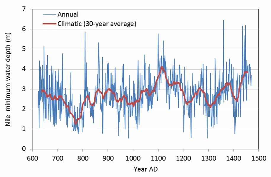
Figure 6.1.1: The annual minimum depth of the Nile River near Cairo over more than 650 years from 622 to 1284 A.D. The data, measured in meters, shows a characteristic pattern of year-to-year fluctuations around longer-term trends. Data from Koutsoyiannis (2013)

A good example of this is the eight-century long record of the annual minimum height of the Nile River observed at Roda Island in Cairo shown in Figure 6.1.1. The Nile River is fed by precipitation over a 4 million square mile drainage basin, an area equal to about one third of CONUS. Since human influences on the global climate were negligible long before the 20th century, the century-scale variability of the thirtyyear average is entirely natural; Egyptians of the seventh and eight centuries would have been incorrect to assume that the worsening drought during that time was the “new normal.”

With these caveats in mind, we examine the evidence for changes in selected weather and climate extremes. A recurring theme is the wide gap between public perceptions and scientific evidence. It has become routine in media coverage, government and private sector discussions, and even in some academic literature to make generalized assertions that extreme weather of all types is getting worse due to GHGs and “climate change.” Yet expert assessments typically have not drawn such sweeping conclusions and instead have emphasized the difficulty both of identifying specific trends and establishing a causal connection with anthropogenic forcing.

In the sections to follow we provide excerpts from various IPCC and NCA assessment reports denoting the sources as follows:

SREX: The IPCC Special Report on Managing the Risks of Extreme Events and Disasters to Advance Climate Change Adaptation (2012)

AR6: The IPCC Sixth Assessment Report Working Group 1 (2021).

NCA4: The U.S. Climate Science Special Report of the Fourth National Climate Assessment (2017) Volume I.

NCA5: Fifth National Climate Assessment (2023).

In the excerpts. italics are in the original whereas boldface emphasis has been added.

Additionally we use standard government sources to provide information through 2024 wherever possible.

6.2 Hurricanes and tropical cyclones

AR6 provides the following assessment of tropical cyclones (TCs; used here as a synonym for hurricanes):

AR6: There is low confidence in most reported long-term(multidecadal to centennial) trends in TC frequency or intensity-based metrics due to changes in the technology used to collect the best-track data. (IPCC, 2021 p. 1585)

AR6: It is likely that the global proportion of major (Category 3–5) tropical cyclone occurrence has increased over the last four decades . . . There is low confidence in long-term (multi-decadal to centennial) trends in the frequency of all-category tropical cyclones. (IPCC, 2023 SPM p. 9)

AR6: A subset of the best-track data corresponding to hurricanes that have directly impacted the United States since 1900 is considered to be reliable, and shows no trend in the frequency of U.S. landfall events (IPCC 2021 p. 1585)

Since 1980, when satellite observations first fully coveredthe global oceans, we have confidence in the numbers of total global hurricanes and major hurricanes (Category 3 and higher). Figure 6.2.1 shows that on average, each year there are about 50 hurricanes, with about 25 reaching major hurricane status (Maue, 2025). There is substantial year-to-year and decadal variability, a weak decrease in the number of hurricanes, and a slight but insignificant increase in the number of major hurricanes These two trends combine to create an overall increase in the proportion of major hurricanes.

Global hurricane statistics are dominated by the Northwest Pacific Ocean, which accounts for ~35 percent of total global hurricanes, whereas the Atlantic accounts for ~15 percent of global hurricanes (Colorado State University, 2025). Data in the Atlantic basin extends further back than in the other ocean basins and is most relevant to U.S. policy makers.

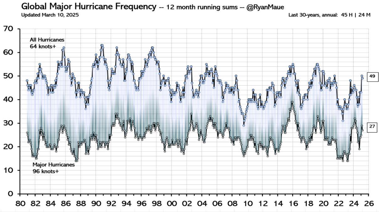
Figure 6.2.1: Global frequency of hurricanes and major hurricanes since 1980. Source: Updated from Maue 2011.

Figure 6.2.2 shows the frequency of Atlantic hurricanes and major hurricanes (Category 3 and higher) back to 1920. Data prior to 1965 (the onset of satellite observations in the Atlantic, shaded in blue) shows some undercounting, with data prior to 1920 showing substantial undercounting (Vecchi and Knutson, 2011). All measures of Atlantic hurricane activity show a significant increase since 1970. However, the period from 1971-1994 saw exceptionally low activity, with high activity (comparable to the past two decades, even with undercounting) also observed during the 1950’s and 1960’s, and even in the 1930’s.

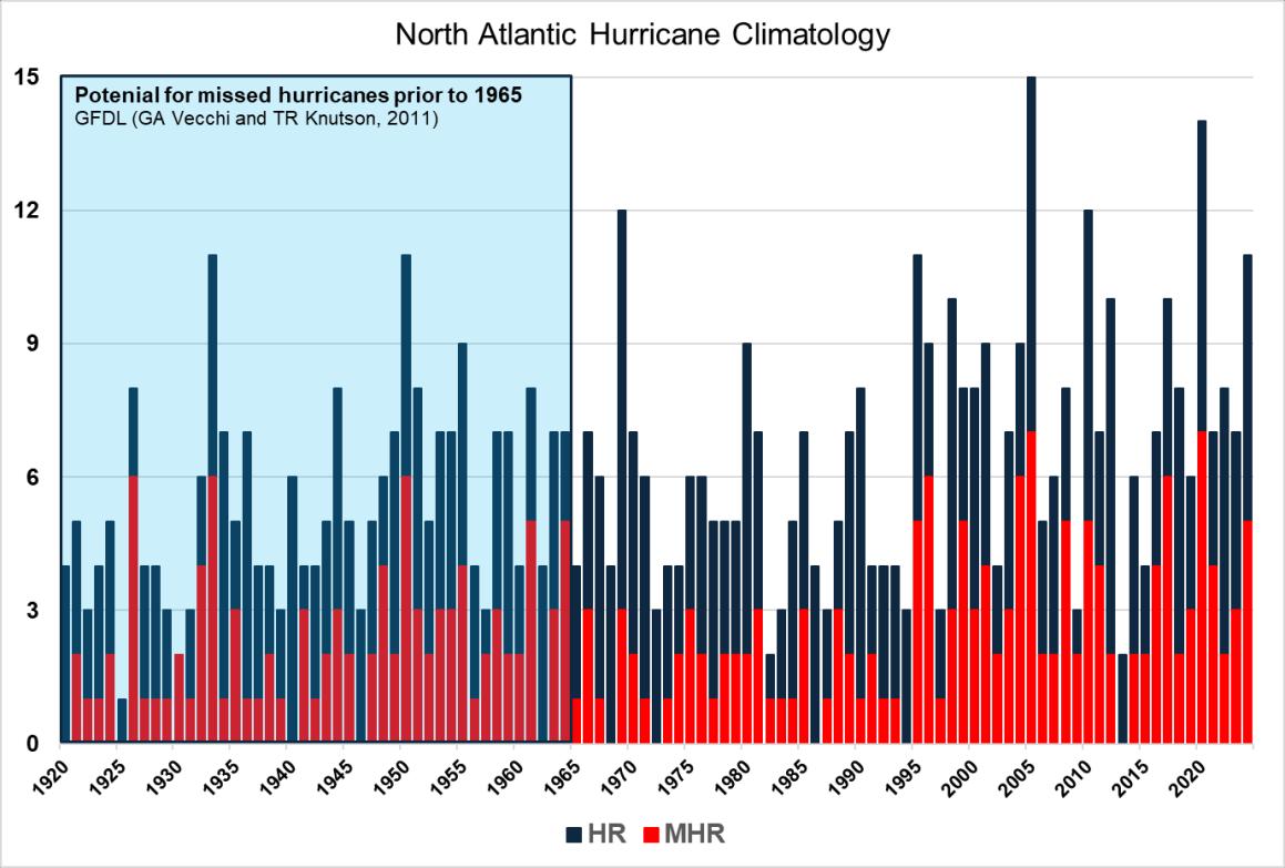
Figure 6.2.2: Atlantic frequency of hurricanes (HR) and major hurricanes (MHR) since 1920. Source National Hurricane Center (2024)

Figure 6.2.2 shows that Atlantic hurricanes vary strongly on decadal and multidecadal time scales. These variations are associated primarily with the Atlantic Multidecadal Oscillation (AMO), which is manifest in basin-wide sea surface temperature and sea level pressure fluctuations connected to large scale ocean circulation patterns. The AMO was in its warm phase during 1926-1970 and 1995-present, but in its cool phase during 1971-1994. It has its greatest impact on the number of major hurricanes (Category 3+), which Goldenberg et al. (2001) associated with above normal SSTs and decreased vertical shear in the AMO warm phase (see also Bell and Chelliah, 2006; Klotzbach et al., 2018).

Klotzbach et al. (2018) conducted a comprehensive evaluation of the landfalling hurricane data for the Continental U.S. since 1900. Figure 6.2.3 updates their analysis through 2024. While the largest numbers of landfalling hurricanesare from2004, 2005 and 2020, there is no statistically significanttrend since 1920.

Figure 6.2.3 also shows the time series for major hurricane landfalls (Category 3-5). The largest year in the record is 2005, with 4 major hurricane landfalls. However, following 2005 there were no major hurricanes striking the U.S through 2016, the longest such period since 1920

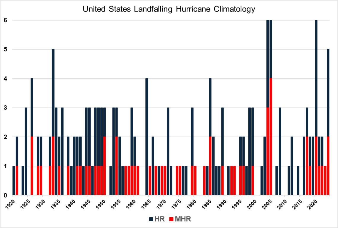
Figure 6.2.3: U.S. landfalling frequency of hurricanes (HR) and major hurricanes (MHR) since 1920.

Source NOAA HRD(a) (2024)

Figure 6.2.3 shows substantial interannual to multidecadal variability in U.S. landfall activity Klotzbach et al. (2018) examined how the landfall counts vary with ENSO (El Niño versus La Niña) and the warm versus cold phases of the Atlantic Multidecadal Oscillation (AMO).

Villarini et al. (2012) provide an analysis of U.S. hurricane landfalls back to 1878. While it is possible that some landfalls were missed in the late 19th century owing to sparsely populated regions on the Gulf Coast, it is remarkable that the highest year in the entire record is 1886, with 7 hurricane landfalls, when human influences on the climate were much smaller than they are today.

Table 6.2.1 shows the 10 strongest hurricanes (plus ties) to make U.S. landfall. Of the hurricanes that have made landfall with sustained winds greater than 150 mph, only one has occurred in the 21st century.

In summary, analyses of both global and regional variability and trends of hurricane activity provide the basis for detecting changes and understanding their causes. The relatively short historical record of hurricane activity, and the even shorter record from the satellite era, is not sufficient to assess whether recent hurricane activity is unusual relative to the background natural variability. Atlantic hurricane processes are influenced substantially by the natural modes of ocean circulation variability in the Atlantic, notably the Atlantic Multidecadal Oscillation. While it has long been hypothesized that a rising global sea surface temperature would cause an increase in hurricane intensity, identification of any significant trend in the hurricane data is hampered by a short data record and substantial natural variability.

Process-based understanding also suggests that storm surges and rainfall from hurricanes should be increasing with warmer temperatures. However, the relatively small number of hurricanes with varying landfall locations and the complex dynamics associated with each storm preclude meaningful detection of change.

Rank

1 1935 185 "Labor Day"

2 1969 175 Camille

3 1992 165 Andrew

4 2018 160 Michael

5 1856 150 "Last Island"

5 1886 150 "Indianola"

5 1919 150

5 1932 150 "Freeport"

5 2004 150 Charley

5 2020 150 Laura

5 2021 150 Ida

5 2022 150 Ian

Table 6.2.1 Strongest hurricanes to make landfall along the U.S. coast. Source (NOAA HRD(b), 2024)

6.3 Temperature extremes

The AR6 assessment focused on the period after 1950 and reported increasing trends in heatwave frequency and intensity. However, NCA4 noted that heatwave activity in the U.S. reached a peak in the 1930s (Figure 6.3.1)

AR6:It is virtually certain that hot extremes(including heatwaves) have become morefrequent and more intenseacrossmostland regions since the 1950s, while cold extremes (including cold waves) have become less frequent and less severe (SPM, A3.1)

AR6: In North America, there is very robust evidence for a very likely increase in the intensity and frequency of hotextremes and decrease in the intensity and frequency of cold extremes for the whole continent, though there are substantial spatial and seasonal variations in the trends. Minimumtemperaturesdisplaywarmingconsistentlyacrossthecontinent,whiletherearemore contrasting trends in the annual maximum daily temperatures in parts of the USA. (Chapter 11, p 1550)

NCA4: Changes in warm extremes are more nuanced than changes in cold extremes. For instance, the warmest daily temperature of the year increased in some parts of the West over the past century, but there were decreases in almost all locations east of the Rocky Mountains. In fact, all eastern regions experienced a net decrease, most notably the Midwest (about 2.2°F [1.2°C]) and the Southeast (roughly 1.5°F [0.8°C]). (pp. 190-191)

NCA4: Since the mid-1960s, there has been only a very slight increase in the warmest daily temperature of the year (amidst large interannual variability). Heat waves (6-day periods with a maximum temperature above the 90th percentile for 1961–1990) increased in frequency until the mid-1930s, became considerably less common through the mid-1960s, and increased in frequency again thereafter. As with warm daily temperatures, heat wave magnitude reached a maximum in the 1930s. (pp. 190-191)

6.3.1 Temperatures in the U.S. are becoming less extreme

Daily maximum temperatures in the warm season (Tmax, May-Sep) and daily minimum temperatures in the cold season (Tmin, Dec-Mar) are available beginning in Dec 1898 (126 years). The dataset consists of 1,211 CONUS stations designated as United States Historical Climate Network or USHCN stations (see Figure 6.3.2; Quinlan et al. 1987, Karl et al. 1990). These stations were selected by NOAA as having the fewest problematic issues with gaps, station moves, and instrument changes. Where gaps still exist, nearby stations (bias-corrected) were merged so that the median volume of data available for a station is 98%. Although therearecertainly errorsin thedataset, includingunresolvedspurious warming due to UHIeffects that especially bias Tmin records, this data set is sufficiently accurate for assessing trends in Tmax heat extremes

Figure 6.3.1: U.S. Heat waves since 1900. Source: NCA4 Figure 6.4

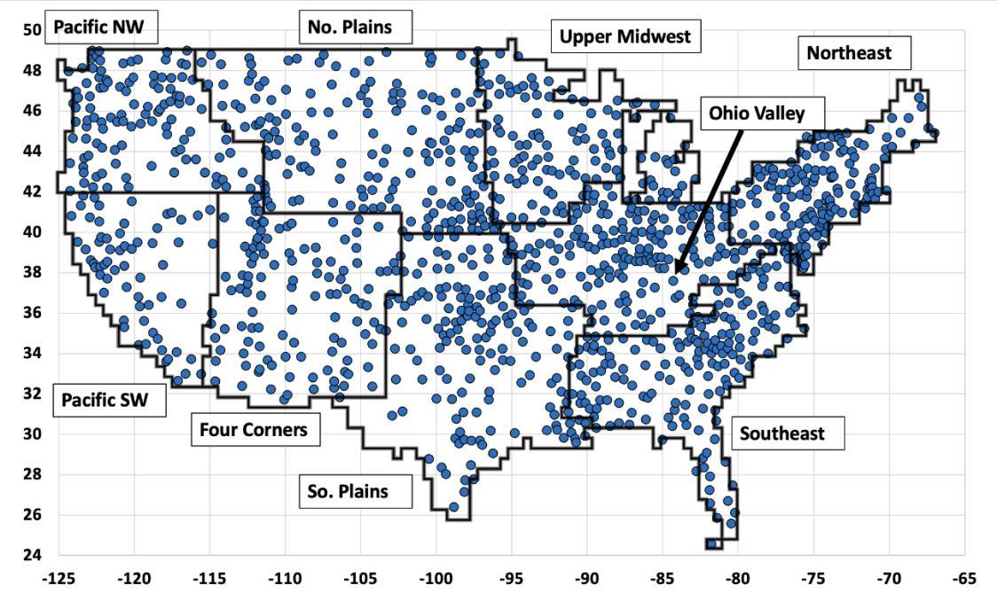
Figure 6.3.2 Locations of USHCN temperature stations. Source: USHCN.

We begin with the question of whether the occurrence of daily record high or low temperatures has changed since Dec 1898. Each warm-season has 153 days (1 May to 30 Sep) and each cold-season has 122 days (1 Dec to 31 Mar). For each station and day, we calculated the year in which the record highest (lowest) temperature occurred. With 126 years of observations, if there were no temperature trends over time, the expected number of records for Tmax would be 1.21 (=153/126) per station per year and for Tmin 0.96 (=122/126) per station per year.

Figure 6.3.3 shows the observed distribution in time of the occurrence of these extreme events. There is a common feature in many metrics of warm-season extremes in the CONUS - the exceptional heat of the 1920s and especially the 1930s, peaking in 1936. On a per-station average, 60 percent of the Tmax records and 59 percent of the Tmin records occurred in the first half of the period (1899-1961).

Figure 6.3.3 Number of daily record High (red) and Low (blue) temperatures for warm and cold seasons in the CONUS. The lines represent the 15-year running, centered average. Source: 1,211 USHCN stations supplemented as needed to achieve a minimum of 92 percent of observations in the 126-year period since Dec 1898. US48: contiguous U.S. states. Tmax: maximum temperature. Tmin: minimum temperature.

On the cold side, the Valentine’s Day Arctic outbreak in Feb 1899 stands as the most extensive cold extreme experienced by CONUS, with 1917 in 2nd place. The frequency of cold records has declined, especially over the last quarter of the period in which only 13 percent of the extreme cold events were measured. In contrast, 25 percent of the extreme Tmax records were achieved in the last quarter, in accordance with statistical expectations. These general features have been noted in past assessments (see above, IPCC AR6, NCA4). Combining the two histories, the overall reduction in numbers of both cold and hot extremes over the past century indicates a climate less prone to extremes.

This pattern is also shown in Figure 6.3.4. For each station and for each year the hottest warm season and coldest cold-season temperatures were calculated. Then the differences between these were computed by station and geographically-averaged over all stations, thus yielding an annual measure of the expected range of local extreme temperatures for each year. Figure 6.3.4 shows the 15-year trailing average of this measure, which has clearly declined over the past century.

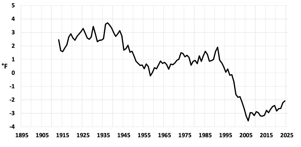
Figure 6.3.4. 15-year trailing average of the difference each year of each station’s hottest warmseason Tmax and coldest cold-season Tmin relative to the long-term average. Source: Author analysis of USHCN data

The average difference for each station between the hottest summer Tmax and coldest winter Tmin has declined by about5°Fin the past126 years. The decline isdue mostly to warmer winter Tmin, but a decline in summer Tmax is also a factor. The rise in Tmin has been strongly related to the growing presence of manufactured surfaces around the weather stations over the last 100+ years (the so-called urban heat island effect; Section 3.3, Karl et al. 1988, Runnals and Oke 2006, and Spencer et al. 2025).

In summary, while temperature extremes are regularly experienced in the U.S. and attract a great deal of media attention, long term records show the U.S. climate has become less extreme over time (milder) when measured by the range between warm season maxima and cold season minima.

6.3.2

Exceedances of a heat threshold

Under the heading of “The Risk of Temperature Extremes is Changing”, the most recent U.S. National Climate Assessment report (NCA5) notes the increase in a threshold metric of number of days at or above 95°F, stating,

The western U.S. has been particularly affected by extreme heat since the 1980s …, experiencing a larger increase in days over 95°F, as would be expected given the greater warming in that region relative to the eastern US. Several major heatwaves have affected the U.S. since 2018, including a record-shattering event in the Pacific Northwest in 2021.

Are the occurrences of 95°F days changing? In a climate as varied as that of CONUS, threshold statistics can be misleading. A region with many stations that have near 95°F Tmax average temperatures in the summer might see large swings in the metric when only small changes in average temperature occur. Elsewhere with stations that either rarely or virtually always achieve 95°F Tmax temperatures, a small change will not have much impact on the results.

Figure 6.3.5. Total number of days ≥ 95°F in 6-yr periods, U.S. 48 (bars) and regions (lines). A 6year period is used as this evenly divides the 126-year record Results are robust to using periods from 2 to 11 days. US48: contiguous U.S. states. See Figure 6.3.2 for region names. Source: Author analysis of USHCN data

In the past 126 years, the average CONUS station experienced 129 days exceeding 95°C per 6-yr period, but the regional values range from 278 in the Southern Plains to 9 in the Northeast. Thus, such threshold analyses must be interpreted with caution. Figure 6.3.5 shows that only three of the nine regions, all in the West, have experienced upward trends in the number of 95°F or hotter days (dashed lines). The CONUS as a whole has not, and the other six regions have experienced declines.

The Pacific NW heatwave of 2021 referenced in the NCA5 quote will be examined more closely in Section 8.6.1. The evidence indicates that it was a single, unprecedented event in the record, not part of a pattern of increasing extreme heat. For example, the 5-day average tropospheric grid-point temperature anomaly over the Pacific NW during that event was +10.8 C, the most extreme Northern Hemisphere grid point summer anomaly in the 46 years from over 4 million grid values. In contrast, the global temperature anomaly during that time was virtually zero (+0.03 C, Mass et al. 2024).

6.3.3

Heatwaves

Heatwaves (consecutive days that exceed an extreme threshold) have a greater societal impact than a single daily record temperature. We measure “Heatwave Days” here as the count of all days in May-Sep each year that exceed the 90th percentile for that day and that lie within a period of at least six consecutive days. This is equivalent to the method used in NCA4, except that the reference period here is the entire record 1899-2024 while NCA4 truncated the reference period to 1961-1990, which was a cool interval. (The pattern of results shown below does not depend on the choice of reference period.) That truncation boosts positive results (days exceeding the 90th percentile) in years warmer than the reference period, especially starting in 1960 and moving to the present (see Figure 6.3.6 and discussion below).

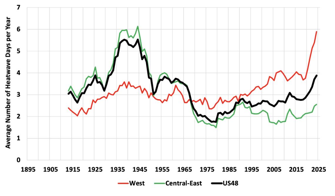
Figure 6.3.6 15-year trailing average of number of heatwave days per year per station in the CONUS (black line) and two regions: West (red), Central-east (green).

Figure 6.3.6 indicates that there are regional variations in heatwave activity. The excessive heat of the first half of the 20th century occurred primarily in the eastern two-thirds of the nation, while the West has seen a recent increase of heatwave days (NCA5). This indicates that the background warm season circulation favored heatwaves in the eastern portions of the country in the first half of the 20th century, but in the 21st century the patterns have favored heatwaves in the West. For CONUS as a whole, heatwaves are no more common today than they were a century ago, consistent with the upper panel of our Figure 6.4.1 taken from NCA4.

This metric varies significantly with region. The four northern regions (Pacific NW, Northern Plains, Upper Midwest, and Northeast) on average experience 15 to 27 heatwave days per 15-year period. In contrast, the five southern regions (Pacific Southwest, 4-Corners, Southern Plains, Ohio Valley and Southeast) see 37 to 54 such days, essentially twice as many. This suggests the summer circulation pattern is more prone to stationary events in the southern regions while transient systems in the northern regions are more common and thus cut short these potentially longer events.

The analysis of heatwaves is an example of why it is important to consider complete datasets and appropriate metrics. The NCA5 directs readers to the website https://www.globalchange.gov/indicators/heat-waves (USGCRP 2023) to view a figure showing the number of urban heatwaves by decade from the 1960s, which we reproduce as Figure 6.3.7.

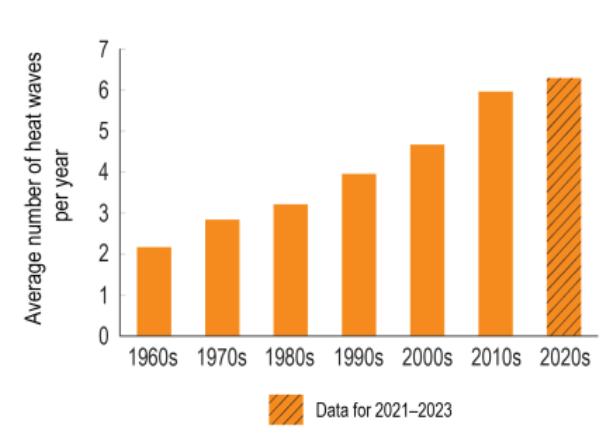
Figure 6.3.7: Average number of urban heatwaves per year for 50 large U.S. metropolitan areas, a misleading metric for reasons explained in the text From https://www.globalchange.gov/indicators/heat-waves (accessed May 22, 2025).

The figure shows a monotonic increase in each decade from two occurrences per year in the 1960s to six in the 2020s. The definition of aheatwave usedis an unusual but practical measure ofhuman discomfort - a period of at least 2 consecutive days when the minimum apparent temperature (combination of temperature and humidity) exceeds the 85th percentile. Note too, the dataset is limited to the 50 largestU.S. cities.

Given the unusual heatwave definition and urban focus, these increasing values since 1960 presented in USGCRP (2023) are not informative about long term trends or the influence of GHG emissions for at least two reasons. First, as shown in Figures 6.3.1 and 6.3.6, the 1960s was the coldest decade and 1970s the second coldest decade since the 1910’s, so this starting date preconditions the time series to show increases. Second, post-1960 urbanization in these cities is a major factor in the rise of Tmin relative to colocated Tmax and relative to Tmin at nearby rural stations (Karl et al. 1988, Runnals and Oke 2006, Christy et al. 2009, McNider et al.2012). This does not dismiss the real rise in nighttime temperatures in major U. S. cities and the societal impacts associated with these changes. However, we note for a variety of reasons that summer Tmax (especially in rural areas) is a better metric for detecting changes in heatwaves influenced by changes in the background climate due, for example, to increasing GHGs (Christy et al. 2009). For CONUS as a whole, the evidence in this section suggests GHG emissions have had little-to-no effect on heatwaves against the background of urbanization and natural climate variability Irrespective of the ultimate cause of regional trends, heatwaves have important effects on society that must be addressed, as we discuss in Chapter 10.

BOX: Perils of short data records

San Francisco provides a good case study of the limitation of using short historical samples to characterize natural variability of extreme events. Suppose we use a 130-year sample of daily San Francisco precipitation from 1895 to 2024 and we look for 3-day, 5-day, 14-day and 30-day rainfall records. The results are as shown in Table 6.2.

Table 6.2: Extreme rainfall records, San Francisco, 1895-2024.

The records all cluster in the more recent years. 2023 appears to be an exceptional year and since it is near the end of the sample, it might suggest that the climate has shifted into a more hazardous state, perhaps because of human influences. [Note “2023” indicates the event occurred in the wateryear of Aug 2022 to Jul 2023.]

But the picture is very different if we use a sample that begins 45 years earlier, in 1850. Table 6.3 shows that the record-setting events all happened in the 1860s. Furthermore 2023 is now not even in 2nd place but falls to 3rd or 4th place. And comparing the records of the two charts shows the extreme precipitation events in 1862 and 1867 involved considerably more rainfall than the 1998 and 2023 events, with 14- and 30-day totals about 50 percent higher.

Table 6.3: Extreme rainfall records, San Francisco, 1850-2024.

The range of natural variability is made even more remarkable when paleoclimate evidence is examined. Porter et al. (2011) discovered that in the past 1,800 years at least six megastorms were more intensethanthe devastating 1861-62 ARkStorm thatstruck theregion. Evidently suchextreme events, “unprecedented” in our 1895-2024 sample, have impacted the region about every 300 years, though not since 1895.

This example illustrates the limitations of using relatively short climate periods (~130 years) to assess the character and range of natural variability in general and of extreme events in particular. Accurate representation of the full range of natural variability is necessary for any attribution analyses (Section 8.6). Infrastructure planners, emergency management institutions and attribution scientists would understand the significant mischaracterization of the magnitude of a future extreme if based only on the last 130 years. In this case, a single time-sample of 130 years provides an underestimation of the extreme value by up to 50 percent determined when adding only 45 more years of observations. Compared to millennial-scale paleoclimate evidence, an even greater underestimation would occur. An important lesson is that the climate can deliver great surprises on its own, even without human influences.

6.4 Extreme precipitation

AR6 assessed that an increase in heavy precipitation has been observed in data starting in the 1950s.

AR6: The frequency and intensity of heavy precipitation events have increased since the 1950s over most land area for which observational data are sufficient for trend analysis (high confidence). (SPM A3.2)

AR6: In North America, there is robustevidence that the magnitude and intensity of extreme precipitation has very likely increased since the 1950s. Both [one-day maxima] and [5-day maxima] have significantly increased in North America during 1950-2018. (Chapter 11, p. 1560)

The U.S. NationalClimate Assessments (NCA4, NCA5) have highlighted an increase in the occurrence of the heaviest precipitation events (defined in different ways) primarily in the eastern half of CONUS, especially the Northeast, when starting the analysis in either 1901 or 1958. Interestingly, the regional variations indicate that the largest increases in extreme precipitation events are in the Northeast and the smallest in the West, a pattern counter to the changes in temperature extremes (Figure 6.3.6).

McKitrick and Christy (2019) examined long-term and consistent station observations of extreme daily precipitation to test some of these NCA claims for the Southeast and West Coast using a trend model with a non-parametric variance estimator robust to the complex autocorrelation properties of precipitation data. When the time series were extended back in time (as far as1872 in some cases) or started later (1978), there were no significant trends for either region.

These findings have been updated for this report (McKitrick and Christy 2025) with similarly constructed observations from 29 stations on the CONUS Pacific Coast (1893ff from San Diego CA to Blaine WA) and 24 stations in the humid Southeast (1872ff from Austin TX to Washington DC), also adding 27 stations in the Northeast (1888ff from Buffalo NY to Eastport ME). The locations are shown in Figure 6.4.1. Thestations were selectedbasedon availability of long-termhigh-quality records. Theregions areeach associated with importantfeatures ofextreme precipitation behavior: the Pacificcoastis associated with landfalling atmospheric rivers for which AR6 cites evidence of increasing activity since 1948 with further increases expected as the world warms (AR6 8.3.2.8.2); the NCA report indicates that the Northeast has experienced the greatestincrease in extreme events, and the Southeastis also a place noted in the NCAs as having increased extreme events.

The results of applying the analysis of McKitrick and Christy (2019) were as follows for each region, then followed by further explanation.

Pacific Coast heavy rainfall events

• The average precipitation trend is statistically significant(downwards) in Astoria OR; insignificant elsewhere.

• The trend in rainfall variance is positive and significant in Big Sur CA; insignificant elsewhere.

• The trend in daily maximum precipitation is positive and significant in Aberdeen WA and Big Sur CA and negative and significant in Newport OR (insignificant elsewhere).

• Averaged over all stations in the region, none of these three trend parameters is statistically significant.

The Pacific Coastreceives considerable precipitation from Atmospheric River (AR)events which often last more than a day or two (e.g., Gershunov et al. 2017, Pan et al. 2024). The worst series of such events in recent history was the so-called ARkStorm that occurred during December 1861 and January 1862; it dumped nearly 10 feet of rain in parts of California and submerged the entire Central Valley for weeks under as much as 15 feet of water (Brewer 1930, Null and Hulbert 2007). Additionally, paleoclimate research has found six megastorms more severe than 1861–1862 in California during the last 1800 years, occurring at intervals of 300 years or so (Porter et al. 2011).

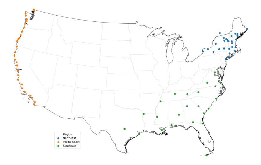
Figure 6.4.1: Locations of precipitation monitoring stations used in this report. Orange: Pacific coast. Blue: Northeast. Green: Southeast. Data from McKitrick and Christy (2025).

We examine occurrences of 5-day deluges as follows. Taking the Pacific coast as an example, a 130year span contains 26 5-year intervals. At each location we computed the 5-day precipitation totals throughout the year and selected the 26 highest values across the sample. A single year might have more than one of the 26 heaviest. Each of those can be thought of as 1-in-5yr events. If there are no trends in precipitation, then the total number of these events across all stations should be evenly spread over the years. In Fig. 6.4 2 we show the distribution in time of these events for the Pacific coast. The deluges associated with the massive 1997-98 El Niño event are readily apparent. While erratic, as is typical of such precipitation metrics, there is no indication of a tendency to become more frequent over time.

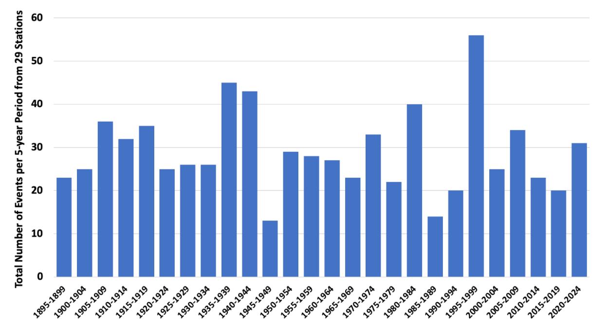
Figure 6.4.2. The time distribution by 5-year periods of the 26 heaviest (1-in-5 yr) occurrences for 29 stations on the Pacific coast.

Figure 6.4.3. As in Fig. 6 4 2 but for the heaviest 30 (1-in-5yr) events for 24 stations in the humid Southeast from Austin TX to Washington DC in 5-year bins for 1875-2024.

Southeast heavy rainfall events

• The trend inaverageprecipitation is positiveand statistically significant in MobileALand Quitman GA but insignificant elsewhere.

• The trend in rainfall variance is positive and significant in Mobile AL but insignificant elsewhere.

• The trend in daily maximum precipitation is positive and significant in Vicksburg MS and Norfolk VA but insignificant elsewhere.

• Averaged over all stations in the region none of these three trend parameters is statistically significant

Figure 6.4.3 is analogous to Figure 6.4.2 for the last 150 years in the Southeast humid zone. The temporal pattern of 5-day totals of the 1-in-5yr heavy events is generally unremarkable, though a cluster of higher values appears in 1995 to 2019. The increase in those years is due largely to the 4 northeastern-most stations of Wilmington NC, Weldon NC, Washington DC, and Norfolk VA. This confirms the pattern indicated in NCA4 and NCA5 an increasing frequency of heavy events due to a temporal clustering of tropical storms from eastern NC to Maine discussed below. Otherwise, the remaining 20 stations show an unremarkable temporal distribution of heavy events.

Northeast heavy rainfall events

• The trend in average precipitation is positive and statistically significant in 12 of 27 locations and also in the regional average.

• The trend in rainfall variance is positive and significant in Portland ME, Albany NY, Buffalo NY and Eastport ME but insignificant elsewhere.

• The trend in daily maximum precipitation is positive and significant in Portland ME, Gardiner ME and Eastport ME but insignificant elsewhere.

• When averaged over all stations in the region, there is no statistically significant trend in either the precipitation variance or maximum

Fig. 6 4 4 is analogous to Figure 6.4.2 for the last 135 years in 27 stations in the Northeast (including Montreal Canada). We use 3-day totals here as this produced the largest temporal variations in time. In this region, 77 percent of events occur during June to October and are dominated by incursions of hurricanes, tropical storms, or tropical storms that transition to extratropical systems. According to NCA4 and NCA5 this region experienced the largestincreases in extremeevents, so itmerits a closer examination.

There is a noticeable clustering of extreme events from 1995 to 2014. Howarth et al. (2019) examined a similar region as in Fig. 6.4.4 that includes PA and NJ and reported significant differences in various precipitation extremes between two 18-year periods, 1979-96 and 1997-2014. That included a 317 percent increase in 24-hr events exceeding 6 inches, while we find a 58 percent increase over the same years. However, Figure 6.4.4 shows that frequency drops sharply after 2014, returning to the long-term average in the subsequent 5-year intervals, again illustrating the perils of drawing conclusions from short-term trends in highly variable metrics.

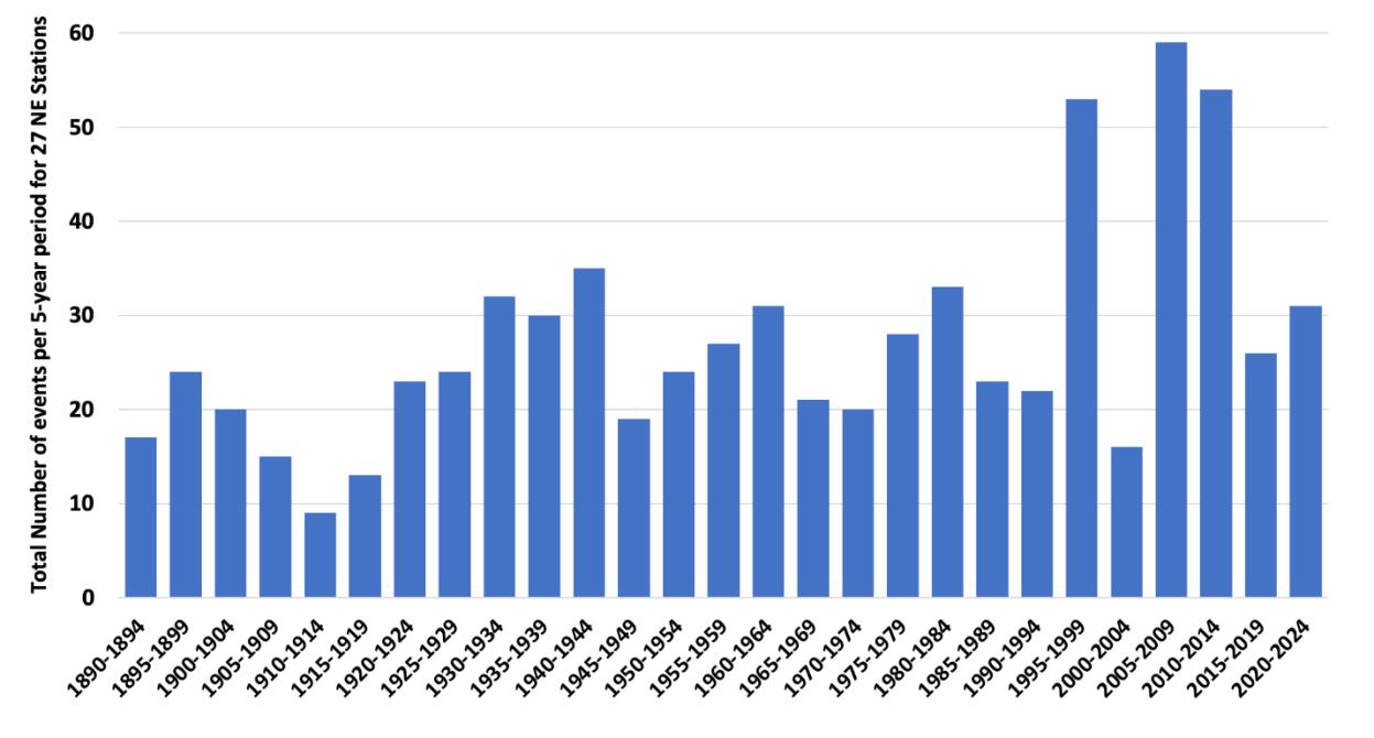
Figure 6.4.4. As in Fig. 6.4.2 but for the heaviest 27 (1-in-5yr) 3-day precipitation events for 27 Northeast stations from NY to ME, including Montreal.

Figure 6.4 5 Average amount of precipitation falling in the 1-in-5yr events for the NE stations.

The high percentage increase in theHowarth et al. sampleis associated with small numbersat relatively few locations: there were only 6 in the first period and 25 in the second across 58 stations. Most of the stations did not record such an event. If there is a region-wide increase in heavy events, it should be seen in the average across allstations. Figure 6.4.5 shows the average precipitation in the 1-in-5 yr events across the NE. The trend is only +0.04 inches/decade. The highest amount, 1935-39, includes the Great New England Hurricane of 1938, one of the rare major (Category 3 or higher) hurricanes to strike the region.

The results in Figs. 6.4.4 and 6.4.5 thus suggest that though there was a surge in the number of events at a few locations during the 1995 to 2014 interval, there was no regional pattern and the change did not persist beyond 2014

Jong et al. (2024) document the increase of tropical influences on precipitation events in the Northeast since 1959 and concluded “The autumn extreme precipitation trend over the Northeast U.S. is primarily attributed to tropical cyclone-related events since the 1990s.” The question then becomes: “Was the temporal clustering of tropical systems in 1997-2014 which affected the Northeast a response to increasing GHGs?” Jong et al. examined CMIP-6 model output which suggests that there will be fewer such systems in the 21st century but that the intensity of the rainfall events might increase. This conjecture is not seen in Fig. 6.4.5 where the amount-per-event has remained steady over the 135-year period.

There is some evidence to indicate the heaviest rainfall events might be redistributed due to the impact of urban infrastructure on the localweather(e.g., PielkeSr. et al. 2011, Zhang et al. 2018, Yang etal. 2024). Yang et al. state “Cities that experience compact development tend to witness larger increases in extreme rainfall frequency over downtown than their rural surroundings, while the anomalies in extreme rainfall frequency diminish for cities with dispersed development.” While this is an important insight to consider, the effect on the specific stations used in this analysis is unknown, or at least not detectable in Fig. 6.4.5.

In summary, some U.S. regions show short-duration increases in extreme precipitation events, consistent with natural variability. But analysis of long term, nationwide historical records that considers the autocorrelation properties of precipitation data does not support the claim that extreme short-duration rainfall events are becoming more frequent or intense.

6.5 Tornadoes

AR6 assesses tornado trends in the U.S. as follows:

[O]bservational trends in tornadoes, hail, and lightning associated with severe convective storms are not robustly detected due to insufficient coverage of the long-term observations. There is medium confidence that the mean annual number of tornadoes in the USA has remained relatively constant. (Chapter 11, section 11.7.3, p. 1594)

The monitoring of weak tornadoes has changed over time. The growth of rural populations and the increasing ability to take video with hand-held devices has led to more frequent reports of weak tornadoes thatproduce minimaldamage.In contrast,strong to violent tornadoeshave been observed more consistently over time. Note that tornado strength is measured by the damage it produces, not by the visual appearance of the funnel. Limited real-time observational capabilities in earlier decades did not prevent identification because strong to violent tornadoes leave much more damage which will be assessed later even if the tornado itself was not observed. Since statistics began in 1950, there has been a substantial decrease (by about 50%) in the number of strong to violent tornadoes as shown in Fig. 6.5.1a.

To summarize, there is a noticeable downward trend in thenumber of severe tornadoes in the U.S. since 1950. After 1990 the number of weak tornadoes in the U.S. has remained roughly constant; data before that are incomplete due to limited monitoring.

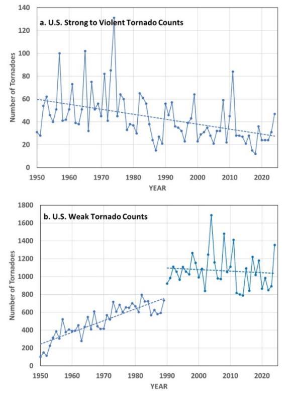
Figure 6.5.1. Annual U.S. tornado counts for (a) strong to violent tornadoes (EF3 to EF5), and (b) weak tornadoes (EF0 to EF2). Based upon NOAA Storms Prediction Center data, available at https://www.spc.noaa.gov/wcm/data/1950-2024_actual_tornadoes.csv

6.6 Flooding

Changes in floods were assessed as follows:

AR6: The SREX assessed low confidence for observed changes in the magnitude or frequency of floods at the global scale. This assessment was confirmed by the AR5 report. The SR15 found increases in flood frequency and extreme streamflow in some regions, but decreases in other regions. . . [H]ydrological literature on observed flood changes is heterogeneous, focusing at regional and sub-regional basin scales, making it difficult to synthesise at the global and sometimes regional scales. (Chapter 11.5)

AR6: [T]he seasonality of floods has changed in cold regions where snowmelt dominates the flow regime inresponseto warming(high confidence). Confidence aboutpeak flowtrends over past decades on the global scale is low. (Chapter 11.5)

NCA4: Trends in extreme high values of streamflow are mixed across the United States. Analysis of 200 U.S. stream gauges indicates areas of both increasing and decreasing flooding magnitude but does not provide robust evidence that these trends are attributable to human influences (pp. 240-241)

The absence of detectable US-wide trends in flooding is consistent with the findings in Section 6.4 of absence of coherent changes in extreme precipitation.

6.7 Droughts

Assessments of drought trends were as follows.

AR6: Few AR6 regions show observed increases in meteorological drought (Section 11.9, p. 1575),

AR6: Increasing trends in agricultural and ecological droughts have been observed on all continents (medium confidence), but decreases only in one AR6 region (medium confidence). Increasing trends in hydrological droughts have been observed in a few AR6 regions. (Chapter 11 Summary)

NCA4: As a consequence of this increased precipitation, drought statistics over the entire CONUS have declined. (p. 233)

NCA4: Recent droughts and associated heat waves have reached record intensity in some regions of the United States; however, by geographical scale and duration, the Dust Bowl era of the 1930s remains the benchmark drought and extreme heat event in the historical record (very high confidence). (p.231)

SREX:Fromapaleoclimateperspective,recentdroughtsarenotunprecedented,withsevere ‘megadroughts’ reported in the paleoclimatic record for Europe, North America, and Australia. (p. 170)

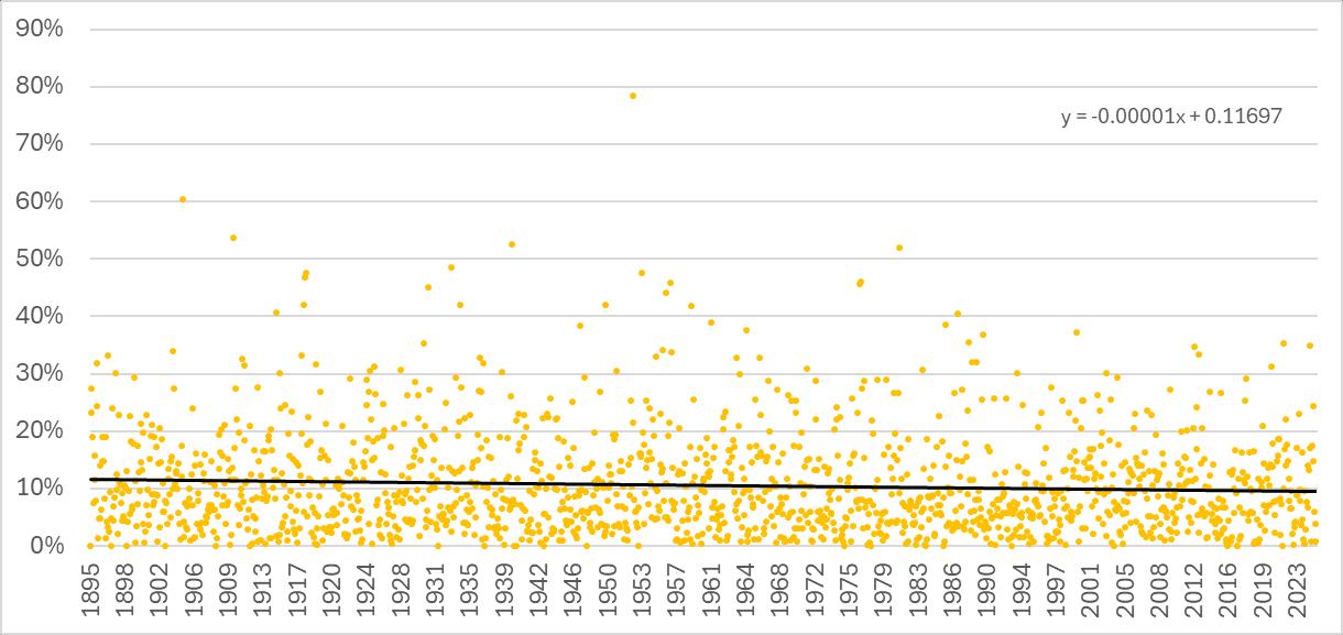
Figure 6.7.1: Monthly percent of US classified as “Very Dry” 1895 2025 Data source: NOAA https://www.ncei.noaa.gov/access/monitoring/uspa/wet-dry/0 least squares trendline added.

As shown in Figure 6.7.1, U.S. long-term data shows an insignificantly declining trend in extreme dryness (-0.001 percent per year)

Kogan et al. (2020) examines a 38-year high-resolution satellite-based drought measure and concludes that global drought has not intensified and is not connected to climate change: “it is possible to state firmly that global and main grain countries’ drought area and intensity trends have not been following global climate warming since 1980’s.”

In summary there is no evidence of increasing meteorological drought frequency or intensity in the U.S. or globally over recent decades.

6.8 Wildfires

The IPCC has not provided an attribution assessment of wildfires. As shown in Figure 6.8.1, global wildfire activity as measured by European Space Agency shows a downward trend in the 21st century.

Figure 6.8.1: Global wildfire area 2001-2018. Source: From Lizundia-Loiola et al. (2021) Figure 12. The different coloured lines represent data products derived from different satellites and algorithms

Global data show that wildfire coverage is constant or declining on every continent (Samborska and Ritchie, 2024). However there is evidence that the intensity of fires in some regions is worsening (Cunningham et al. 2024) and that wildfires resulted in a net loss of global forest cover over 2001-2019 (Tyukavina et al. 2022).

Active fire suppression since 1900 makes it difficult to establish a natural baseline for wildfire activity in the U.S. Paleoclimatic evidence indicates that past activity was much higher than today. Marlon et al. (2012) used sedimentary charcoal layers to reconstruct fire history of western U.S. for the past 1400 years and also fita modelto predict fireactivity as a function ofclimatic conditions. Their results are summarized in Figure 6.8.2 below (from Figure 2 in their paper). There has been a growing wildfire deficit over the 20th century. In other words, however much fire was observed in the 20th century, it was less than what would have been observed in previous centuries based on the climatic conditions. Parks et al. (2025) likewise find that despite the recent increase in wildfire burn area in North America, a significant wildfire deficit remains relative to historical wildfire regimes.

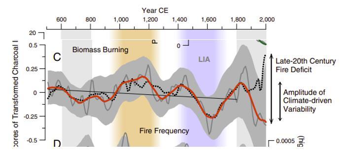
Figure 6.8.2 Fire frequency and fire deficit in the US. The red line shows the smoothed charcoal record and the black dotted line shows the predicted charcoal record based climatic conditions. model. Source: Marlon et al. (2012) Figure 2.

U.S. data from the National Interagency Fire Centre (NIFC) from 1926 to 2023 are shown in Figure 6.8.3. The NIFC has removed the pre-1960 data from its current website on the grounds that measurement methods changed after 1960 making the comparison unreliable. Nonetheless just focusing on the post-1985 interval the number of fires is not increasing. The area burned did increase but only until about 2007.

Forest fires have always been a part of nature, and they can certainly create conditions that are inhospitable in the short term for all life, including humans. Science has confirmed the overall benefit and necessity of forest fires. While recent high-profile fires and seasons serve as a reminder of the potential destructive impact, the highest profile U.S. forest fire remains the 1910 Big Blowup fire in the U.S. west, which destroyed over three million acres and eliminated entire towns like Taft, MT (Apple, 2020). The 1910 fire reshaped the U.S. Forest Service (National Forest Foundation 2022) leading to a focus on fire suppression with a primary goal of defeating all forest fires (Forest History Society, 2022). This led to the “10 am rule” in 1935 requiring that all fires spotted on any day had to be controlled by 10 am the following day (National Forest Foundation, 2022)

While defeating all fires seemed a noble goal, questions began to arise as to whether this behavior “followed the science” (U.S. Forest Service, 2022). Over time the U.S. Forest Service has begun to rethink its goals, recognizing that new approaches such as prescribed burns, fuel elimination, and controlled wildfires aremoreappropriate(Sommer, 2016).Recentresearch is validating this approachand recognizing that more frequent smaller fires likely result in healthier forests, water ecosystems and biodiversity (Stephens et al., 2021).

Figure 6.8.3: U.S. wildfires 1926 to 2023. Source: Post-2018: National InterAgency Fire Center data https://www.nifc.gov/fire-information/statistics/wildfires. Pre-2017 webarchive.org (n.d.).

References

Apple, C. (2020, January 21). 1910 fire – The big burn across Montana and Idaho. The SpokesmanReview https://www.spokesman.com/stories/2020/jan/19/1910-fire-big-burn-across-montana-andidaho/

Bell, Gerald D. and Muthuvel Chelliah, “Leading Tropical Modes Associated with Interannual and Multidecadal Fluctuations in North Atlantic Hurricane Activity,” Journal of Climate 19, no. 4 (February 15, 2006): 590–612, https://doi.org/10.1175/JCLI3659.1

Brewer, W. H. (1930). Up and down California in 1860–1864: The journal of William H. Brewer University of California Press.

Christy, J. R., Norris, W. B., and McNider, R. T. (2009). Surface temperature variations in East Africa and possible causes. Journal of Climate, 22(12), 3342–3356. https://doi.org/10.1175/2008JCLI2726.1

Cohn, T. A. and Lins, H. F. (2005). Nature’s style: Naturally trendy. Geophysical Research Letters, 32(23). https://doi.org/10.1029/2005GL024476

Colorado State University. (2025). Realtime tropical cyclone guidance https://tropical.atmos.colostate.edu/Realtime/index.php

Cunningham, C.X., G.J. Williamson, and D. Bowman (2024) Increasing frequency and intensity of the most extreme wildfires on Earth. Nature Ecology and Evolution 8, 1420–1425 https://doi.org/10.1038/s41559-024-02452-2

Forest History Society (2022). The 1910 fires https://foresthistory.org/research-explore/us-forest-servicehistory/policy-and-law/fire-u-s-forest-service/famous-fires/the-1910-fires/ Gershunov, A., and K. Guirguis (2012). California heat waves in the present and future. Geophysical Research Letters, 39(18). https://doi.org/10.1029/2012GL052979

Gershunov, A., T. Shulgina, F.M. Ralph, D.A. Lavers J.J. and Rutz (2017). Assessing the climate-scale variability of atmospheric rivers affecting western North America. Geophysical Research Letters, 44(15), 7900–7908. https://doi.org/10.1002/2017GL074175

Goldenberg, Stanley et al., “The Recent Increase in Atlantic Hurricane Activity: Causes and Implications,” Science 293, no. 5529 (July 20, 2001): 474–479, https://doi.org/10.1126/science.1060040.

Howarth, M. E., C.D. Thorncroft, and L.F. Bosart (2019). Changes in extreme precipitation in the Northeast United States: 1979–2014. Journal of Hydrometeorology, 20(4), 673–689. https://doi.org/10.1175/JHM-D-18-0155.1

Hurst, H. E. (1951). Long term storage capacities of reservoirs. Transactions of the American Society of Civil Engineers, 116, 776–808.

Intergovernmental Panel on Climate Change (IPCC). (2021). Climate change 2021: The physical science basis. Contribution of Working Group I to the Sixth Assessment Report of the Intergovernmental Panel on Climate Change (V. Masson-Delmotte et al., Eds.). Cambridge University Press. https://www.ipcc.ch/report/ar6/wg1/

Jong, B.-T., H. Murakami, T.L. Delworth and W.F. Cooke (2024). Contributions of tropical cyclones and atmospheric rivers to extreme precipitation trends over the Northeast US. Earth’s Future, 12, e2023EF004370. https://doi.org/10.1029/2023EF004370

Karl, T.R., H.F. Diaz, and G. Kukla. (1988): Urbanization: Its detection and effect on the United States climate record. Journal of Climate, 1, 1099-1123

https://journals.ametsoc.org/view/journals/clim/1/11/15200442_1988_001_1099_uidaei_2_0_co_2.xml

Karl, T. R., C.N. Williams Jr., F.T. Quinlan, and T.A. Boden (1990). United States Historical Climatology Network (HCN) serial temperature and precipitation data (Publication No. 3404). Oak Ridge National Laboratory.

Klotzbach, Phil et al. (2018) Continental U.S. Hurricane Landfall Frequency and Associated Damage: Observations and Future Risks, Bulletin of the American Meteorological Society 99, no. 7 (July 2018): 1359–1376, https://doi.org/10.1175/BAMS-D-17-0184.1.

Kogan, Feliz, Wei Guob and Wenze Yang (2020) “Near 40-year drought trend during 1981-2019 earth warming and food security” Geomatics, Natural Hazards and Risk Vol 11(1)

Koutsoyiannis, D. (2013) Hydrology and Change. Hydrological Sciences Journal 58(6) http://dx.doi.org/10.1080/02626667.2013.804626

Lizundia-Loiola, J., et al. (2020) A spatio-temporal active-fire clustering approach for global burned area mapping at 250 m from MODIS data. Remote Sensing of the Environment 236, 111493, https://doi.org/10.1016/j.rse.2019.111493

Markonis, Y., and D. Koutsoyiannis (2016). Scale-dependence of persistence in precipitation records. Nature Climate Change, 6, 399–401. https://doi.org/10.1038/nclimate2894

Marlon, Jennifer, Patrick J Bartlein, Daniel G. Gavin et al. (2012) Long-term perspective on wildfires in the western USA Proceedings of the National Academy of Sciences February 14 2012 https://www.pnas.org/doi/pdf/10.1073/pnas.1112839109

Maue, R. N. (2025). Climatlas: Tropical cyclones. https://climatlas.com/tropical/ Maue, R. N. (2011) Recent historically low tropical cyclone activity. Geophysical Research Letters 38, L14803, doi:10.1029/2011GL047711

McKitrick, R., and J.R. Christy (2019). Assessing changes in US regional precipitation on multiple time scales. Journal of Hydrology, 578, 124074. https://doi.org/10.1016/j.jhydrol.2019.124074

McKitrick, R. and J.R. Christy (2025), “Data and Code for CWG2025 Report”, Mendeley Data, V1, doi: 10.17632/by76s7rxfb.1

McNider, R.T., G.J. Steeneveld, A.A.M. Holtslag, R.A. Pielke Sr., S. Mackaro, A. Pour-Biazar, J. Walters, U. Nair, and J.R. Christy, 2012: Response and sensitivity of the nocturnal boundary layer over land to added longwave radiative forcing. Journal of Geophysical Research., 117, D14106, doi:10.1029/2012JD017578.

Null, J. and J. Hulbert, “California Washed Away: The Great Flood of 1862,” Weatherwise 60, no. 1 (2007): 26–30, https://doi.org/10.3200/wewi.60.1.26-30

National Forest Foundation. (2022). Blazing battles: The 1910 fire and its legacy https://www.nationalforests.org/our-forests/your-national-forests-magazine/blazing-battles-the-1910fire-and-its-legacy

National Interagency Fire Center. (2024). Wildfire statistics. https://www.nifc.gov/fireinformation/statistics/wildfires

NCA4. (2017). Climate science special report: Fourth National Climate Assessment, Volume I (D. J. Wuebbles, D. W. Fahey, and K. A. Hibbard, Eds.). U.S. Global Change Research Program. https://doi.org/10.7930/J0J964J6

NCA5. (2023). Fifth National Climate Assessment (A. R. Crimmins et al., Eds.). U.S. Global Change Research Program. https://doi.org/10.7930/NCA5.2023.CH1 (accessed May 22, 2025)

NOAA Hurricane Research Division. (2025a). All U.S. hurricanes (1851–2019) https://www.aoml.noaa.gov/hrd/hurdat/All_U.S._Hurricanes.html

NOAA Hurricane Research Division. (2025b). Most intense (3, 4, 5) continental United States hurricanes: 1851–1970, and 1983–2023 https://www.aoml.noaa.gov/hrd/hurdat/most_intense.html

Overland, J. E. (2021). Causes of the record-breaking Pacific Northwest heatwave, late June 2021. Atmosphere, 12(11), 1434. https://doi.org/10.3390/atmos12111434

Pan, M., M. Lu and U. Lall (2024). Diversity of cross-Pacific atmospheric river main routes. Communications Earth and Environment, 5, 378. https://www.nature.com/articles/s43247-02401552-y

Parks, Sean, Christopher Guiterman, Ellis Margolis et al. (2025) A fire deficit persists across diverse North American forests despite recent increases in area burned. Nature Communications 16 https://www.nature.com/articles/s41467-025-56333-8

Pielke, R. A., et al. (2011). Land use/land cover changes and climate: Modeling analysis and observational evidence. Wiley Interdisciplinary Reviews: Climate Change, 2, 828–850. https://doi.org/10.1002/wcc.144

Porter, K., et al. (2011). Overview of the ARkStorm scenario. U.S. Geological Survey. Quinlan, F. T., T. R. Karl, and C.N. Williams Jr. (1987). United States Historical Climatology Network (USHCN) serial temperature and precipitation data (NDP-019). Oak Ridge National Laboratory. Runnalls, K.E. and T.R. Oke, 2006: Technique to detect microclimate inhomogeneities in historical records of screen-level air temperature. Journal of Climate, 19, 959-978. https://doi.org/10.1175/JCLI3663.1

Samborska, V., and H. Ritchie (2024). Wildfires. Our World in Data. https://ourworldindata.org/wildfires

Seneviratne, S. et al. (2021) “Chapter 11: Weather and Climate Extreme Events in a Changing Climate.”

In Climate Change 2021: The Physical Science Basis. Contribution of Working Group I to the Sixth Assessment Report of the Intergovernmental Panel on Climate Change, edited by V. MassonDelmotte, P. Zhai, A. Pirani, S.L. Connors, C. Péan, S. Berger, N. Caud, et al., 1513–1766. Cambridge: Cambridge University Press, 2021. https://doi.org/10.1017/9781009157896.013.

Sommer, L. (2016, November 7). Let it burn: The Forest Service wants to stop putting out some fires. KQED https://www.kqed.org/science/1134217/let-it-burn-the-forest-service-wants-to-stop-puttingout-some-fires

Stephens, Scott et al., (2021) “Fire, Water, and Biodiversity in the Sierra Nevada: A Possible Triple Win,” Environmental Research Communications 3, no. 8 (August 6, 2021): p. 081004, https://doi.org/10.1088/2515-7620/ac17e2.

Tyukavina Alexandra , Peter Potapov, Matthew Hansen et al. (2022) Global Trends of Forest Loss Due to Fire From 2001 to 2019, Frontiers in Remote Sensing. Volume 3 https://www.frontiersin.org/journals/remote-sensing/articles/10.3389/frsen.2022.825190/full U.S. Forest Service. (2022). Managing fire https://www.fs.usda.gov/science-technology/fire USGCRP. (2023). USGCRP indicators platform: Heat waves https://www.globalchange.gov/indicators/heat-waves

Vecchi, Gabriel A. and Thomas R. Knutson (2011) “Estimating Annual Numbers of Atlantic Hurricanes Missing from the HURDAT Database (1878–1965) Using Ship Track Density,” Journal of Climate 24, no. 6 (2011): 1736–1746, https://doi.org/10.1175/2010JCLI3810.1

Villarini, Gabriele, Gabriel A. Vecchi, and James A. Smith, “U.S. Landfalling and North Atlantic Hurricanes: Statistical Modeling of Their Frequencies and Ratios,” Monthly Weather Review 140, no. 1 (January 2012): 44–65, https://doi.org/10.1175/MWR-D-11-00063.1.

Web Archive. (n.d.). Archive of NIFC fire data https://web.archive.org/web/20200212033452/https://www.nifc.gov/fireInfo/fireInfo_stats_totalFires. html

Yang, L., Y. Yang, Y. Shen, et al. (2024). Urban development pattern’s influence on extreme rainfall occurrences. Nature Communications, 15, 3997. https://doi.org/10.1038/s41467-024-48533-5

Zhang, W., G. Villarini, G.A. Vecchi, and J.A. Smith, J. A. (2018). Urbanization exacerbated the rainfall and flooding caused by Hurricane Harvey in Houston. Nature, 563, 384–388. https://doi.org/10.1038/s41586-018-0676-z

7

CHANGES IN SEA LEVEL

Chapter Summary

Since 1900, global average sea level has risen by about 8 inches. Sea level change along U.S. coasts is highly variable, associated with local variations in processes that contribute to sinking and also with ocean circulation patterns. The largest sea level increases along U.S. coasts are Galveston, New Orleans, and the Chesapeake Bay regions - each of these locations is associated with substantial local land sinking (subsidence) unrelated to climate change.

Extreme projections of global sea level rise are associated with an implausible extreme emissions scenario and inclusion of poorly understood processes associated with hypothetical ice sheet instabilities. In evaluatingAR6 projections to 2050 (with reference to the baseline period 1995-2014), almost half of the interval has elapsed by 2025, with sea level rising at a lower rate than predicted. U.S. tide gauge measurements reveal no obvious acceleration beyond the historical average rate of sea level rise.

7.1 Global sea level rise

Global sea level rise is arguably the most important climate impact driver that is unambiguously associated with increasing temperatures. At the global level, warming raises sea level through thermal expansion of sea water and through melting of glaciers and ice sheets. Variations in land water storage are another important factor. At the regional scale, sea level change is influenced by large-scale ocean circulation patterns, and geologic processes and deformation from the redistribution of ice and water Locally, vertical land motion from geologic processes, ground water withdrawal, and fossil fuel extraction are also important.

AR6 estimates that global mean sea level increased by 7.9 (5.9–9.8) inches between 1901 and 2018, with the rate of sea level rise accelerating in recent decades. At the ocean basin scale, sea levels have risen fastest in the Western Pacific and slowest in the Eastern Pacific over the period 1993–2018 (Fox-Kemper et al., 2021). The rate of global sea level rise is estimated to be 0.12 inches/year, about the height of two stacked pennies (NASA, 2020).

The observing systems for global sea level rise have advanced significantly in the satellite era, particularly with the advent of satellite altimeters in 1993. Local tide gauges have provided useful data for the past century, and even longer for a few locations. Following the end of the Little Ice Age in the midnineteenth century, tide gauges show that the global mean sea level began rising during the period 1820–1860, well before most anthropogenic greenhouse gas emissions.

7.2 U.S. sea level rise

Observed and predicted rates of mean global sea level rise might have little scientific relevance for specific locations, owing to local processes (NOAA, 2025). Figure 7.1 shows that in Canada and Alaska (and also northern Washington), sea level is decreasing, owing to uplift from glacial rebound. Most of the Pacific coast tide gauges show low rates of sea level rise, while largest U.S. rates are on the Gulf coast (Louisiana and Texas) and in the mid-Atlantic states (Chesapeake Bay region).

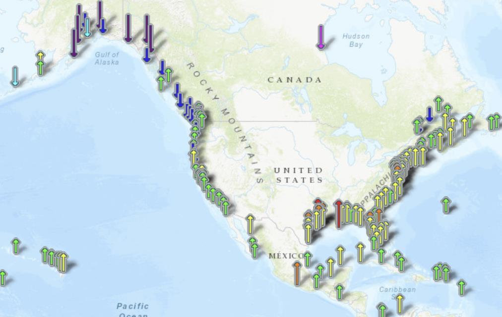
Figure 7.1. Map of rates of relative sea level rise along the U.S. coast (NOAA, https://tidesandcurrents.noaa.gov/sltrends/). For reference, 3 mm = 0.12 in.

Measurements of relative sea level rise from tide gauges conflate the climatologically relevant increase in the volume of seawater with local vertical land motion. The latter, which varies from place to place, is best measured using a Global Positioning System (GPS) station located near the tide gauge. It is driven by a range of processes that can be comparable to the climate signal and can locally exacerbate (subsidence/sinking) or mitigate (uplift) the risk of sea level rise (Wöppelmannand Marcos, 2016). Human activities triggering subsidence are often significant. They include soil drainage (e.g. for urban development) and subsurface extraction of groundwater or hydrocarbons

Table 7.1 shows absolute sea-level rise (ASLR) for selected locations, determined from the sum of uncorrected relative sea-level rise (RSLR) as estimated from tide gauge time series (NOAA, 2025) and the vertical land motion (VLM) measurements (NAS, 2012; Letetrel et al., 2015; Karegar et al., 2016). The absolute sea level rise for each of these locations is significantly smaller than the measured relative sea level rise owing to local subsidence. More than half of the measured relative sea level rise is attributed to land sinking for these locations: San Francisco, Galveston, Grand Isle. For reference, the global average rate of absolute sea level rise is estimated to be 0.12 inches/year.

Francisco, CA

TX

Isle, LA

St Petersburg, FL

New York City, NY

Table 7.1 Absolute sea level rise (inches/year) consisting of Relative Sea Level Rise (RSLR) plus Vertical Land Motion (VLM)

San Francisco Bay

Over the past 100 years, relative sea level in the San Francisco Bay area has risen by 7.8 inches, at an average rate of 0.08 inches/year (Figure 7.2). As shown in Table 7.1, San Francisco’s vertical land motion is -0.06 inches/year (sinking), producing a recent absolute rate of +0.02 inches/year. Portions of Treasure Island, San Francisco International Airport, and Foster City are sinking as fast as 0.4 inches/year (Shirzaei and Bürgmann, 2018). Problems in the San Francisco Bay area, including threats to the airport, are caused primarily by soil compaction in landfill zones that were formerly wetlands, not by the slow creep of global sea level rise.

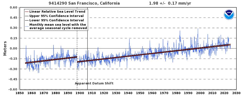
Figure 7.2. Tide gauge measurements at San Francisco, California, obtained from NOAAhttps://tidesandcurrents.noaa.gov/sltrends/sltrends_station.shtml?id=9414290 (downloaded 4/22/25).

Galveston - Houston

Long-term tide measurements at Galveston Pier 21 show sea level rise of 2.18 feet in the past century, or a rate of 0.26 inches/year (Figure 7.3). Vertical land motion (subsidence) at Galveston is estimated at -0.19 inches/year, yielding an absolute rate of rise of +0.07 inches/year (Table 7.1). The U.S. Geologic Survey found that most of the land-surface subsidence in the Houston-Galveston region is a direct result of groundwater withdrawals (Kasmarek and Ramage 2017), which caused compaction of the aquifer sediments, mostly in the fine-grained silt and clay layers. By 1979, as much as 10 feet of subsidence had occurred in Houston.

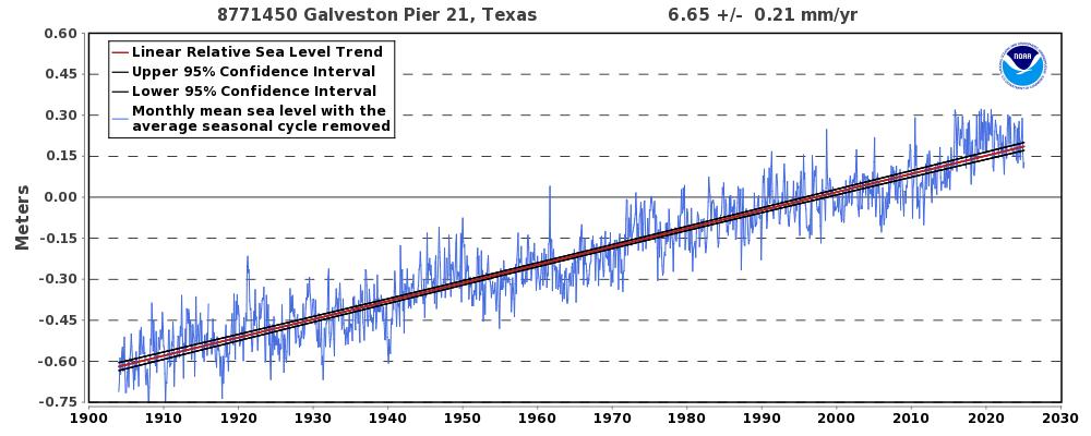
Figure 7.3. Tide gauge measurements Galveston Pier, TX, obtained from NOAAhttps://tidesandcurrents.noaa.gov/sltrends/sltrends_station.shtml?id=8771450 (downloaded 4/22/2025).

New Orleans and the Mississippi delta

Long-term tide gauge measurements at Grand Isle, Louisiana, show that sea level has risen by slightly more than 3 feet over the last 100 years at an average rate of 0.36 inches/year (Figure 7.4). Vertical land motion (subsidence) is estimated -0.28 inches/year. Table 7.1 gives the absolute sea level rise as +0.08 inches/year.

Figure 7.4. Tide gauge measurements at Grand Isle, LA, obtained from NOAAhttps://tidesandcurrents.noaa.gov/sltrends/sltrends_station.shtml?id=8761724 (downloaded 4/22/25).

The issues of sea level rise and land loss in the Mississippi Delta region are complex, with geological subsidence and the decline in sediment transported by the Mississippi River being the dominant drivers. The construction of dams in the basin since the 1950s has decreased the Mississippi’s suspended sediment load by ~50 percent (Maloney 2018). A new subsidence map of coastal Louisiana finds the coastal region to be sinking at about one third of an inch per year (Neinhuis et al. 2017), associated with groundwater and resource withdrawal. As the city’s elevation averages one to two feet below sea level, sea level rise from anthropogenic warming is hardly the dominant driver of New Orleans’ problems.

New York City

New York City is particularly vulnerable to the effects of sea level rise because it is built primarily on islands and has 520 miles of coastline. Measurements by a tide gauge at the southern tip of Manhattan (The Battery) show that relative sea level has risen over 11 inches over the past century, at an average rate of 0.11 inches/year (Figure 7.5). But vertical land motion in the New York City area is -0.05 inches/year (roughly 5 inches per century), so that the absolute rate of sea level rise at The Battery is 0.06 inches/year, or about 55 percent of the measured relative sea level rise.

Figure 7.5. Tide gauge measurements at The Battery, New York, obtained from NOAAhttps://tidesandcurrents.noaa.gov/sltrends/sltrends_station.shtml?id=8518750 (downloaded 4/22/25).

7.3 Projected sea level rise

The concern over sea level rise is not about the roughly eight inches of global rise since 1900. Rather, it is about projections of accelerated rise based upon simulations of a warming climate through the 21st century

AR6 finds high agreement across published global mean sea level projections for 2050 with little sensitivitytoemissionsscenarios. Considering only projections incorporating ice-sheet processes in whose quantification there is atleast medium confidence, the globalsea levelprojections for 2050, across all emissions scenarios, fall between 3.94 and 15.75 inches (5th–95th percentile very likely range) relative to the 1995–2014 baseline period (Fox-Kemper et al., 2021).

Conversely, AR6 states there is low agreement acrosspublished global mean sea levelprojections for 2100, particularly for higher emissions scenarios. Considering only projections representing ice sheet processes in whose quantification there is at least medium confidence, the AR6 global mean sea level projections for2100lie between7.9and 39.4inches(5th–95th percentile very likely range)underthemediumemissions scenario SSP2–4.5 (Fox-Kemper et al., 2021). There is deep uncertainty surroundingprojectionsofsealevel rise to 2100 owing to uncertainties in ice sheet instabilities, particularly for the higher emissions scenarios.

In February 2022, NOAA issued its projections of sea level rise for various sites along the U.S. coast (Sweet et al., 2022). They claim that by 2050, the sea will have risen one foot at The Battery in Manhattan (relative to 2020). A one-foot rise in thirty years would be more than twice the current rate and about three times the average rate over the past century. In that historical context, NOAA’s projection is remarkable as shown in Figure 7.6, it would require a dramatic acceleration beyond anything observed since the early 20th century. But even more noteworthy is that Sweet et al. (2022) say this rise is “locked in” it will happen no matter what future emissions are. We should know in a decade or so whether that prediction has legs.

Figure 7.6 Rate of sea level rise at the Battery in Manhattan. Shown is the historical thirty-year trailing trend, together with the allegedly “locked in” NOAA predicted trend for 2050. Historical data: NOAA Tides and Current.

References

Fox-Kemper, B., Hewitt, H. T., Xiao, C., Adalgeirsdóttir, G., Drijfhout, S. S., Edwards, T. L., ... & Yu, Y. (2021). Ocean, cryosphere and sea level change. In Climate Change 2021: The Physical Science Basis. Contribution of Working Group I to the Sixth Assessment Report of the Intergovernmental Panel on Climate Change (pp. 1211–1362). Geneva, Switzerland: Intergovernmental Panel on Climate Change.

Karegar, M. A., Dixon, T. H., & Engelhart, S. E. (2016). Subsidence along the Atlantic Coast of North America: Insights from GPS and late Holocene relative sea level data. Geophysical Research Letters, 43(7), 3126–3133. https://doi.org/10.1002/2016GL068015

Kasmarek, M. C., & Ramage, J. K. (2017). Water-level altitudes 2017 and water-level changes in the Chicot, Evangeline, and Jasper aquifers and compaction 1973–2016 in the Chicot and Evangeline aquifers, Houston-Galveston Region, Texas (Scientific Investigations Report 2017–5080). U.S. Geological Survey. https://doi.org/10.3133/sir20175080

Letetrel, C., Becker, M., Llovel, W., & Cazenave, A. (2015). Estimation of vertical land movement rates along the coasts of the Gulf of Mexico over the past decades. Continental Shelf Research, 111(Part A), 42–51. https://doi.org/10.1016/j.csr.2015.10.018

Maloney, J. M., Bentley, S. J., Xu, K., Obelcz, J., Georgiou, I. Y., & Miner, M. D. (2018). Mississippi River subaqueous delta is entering a stage of retrogradation. Marine Geology, 400, 12–23. https://doi.org/10.1016/j.margeo.2018.03.001

National Academy of Science (NAS, 2012). Sea-level rise for the coasts of California, Oregon and Washington: Past, present, and future. Appendix A: Vertical land motion and sea-level data along the West Coast of the United States. National Academies Press. https://nap.nationalacademies.org/catalog/13389/sea-level-rise-for-the-coasts-of-california-oregonand-washington

NASA. (2020). NASA sea level rise portal: 2020 edition. https://www.nasa.gov/specials/sea-level-rise2020/

National Oceanic and Atmospheric Administration (NOAA) Center for Operational Oceanographic Products and Services. (n.d.). Sea level trends. https://tidesandcurrents.noaa.gov/sltrends/ NOAA Tides & Currents. (n.d.). Relative sea level trends. https://tidesandcurrents.noaa.gov/sltrends/ Nienhuis, J. H., Törnqvist, T. E., Esposito, C. R., Liang, M., & Ma, H. (2017). A new subsidence map for coastal Louisiana. GSA Today, 27(6), 28–29. https://doi.org/10.1130/GSATG337GW.1 Shirzaei, M., & Bürgmann, R. (2018). Global climate change and local land subsidence exacerbate inundation risk to the San Francisco Bay Area. Science Advances, 4(3), eaap9234. https://doi.org/10.1126/sciadv.aap9234

Sweet, W. V., Hamlington, B. D., Kopp, R. E., et al. (2022). Global and regional sea level rise scenarios for the United States (USGS Report 70229139). United States Geological Survey. https://www.usgs.gov/publications/global-and-regional-sea-level-rise-scenarios-united-states Wöppelmann, G., & Marcos, M. (2016). Vertical land motion as a key to understanding sea level change and variability. Reviews of Geophysics, 54, 64–92. https://doi.org/10.1002/2015RG000502

8 UNCERTAINTIES IN CLIMATE CHANGE ATTRIBUTION

Chapter summary

“Attribution” refers to identifying the cause of some aspect of climate change, specifically with reference to anthropogenic activity. There is an ongoing scientific debate around attribution methods, particularly regarding extreme weather events. Attribution is made difficult by high natural variability, the relatively small expected anthropogenic signal, lack of high-quality data, and reliance on deficient climate models. The IPCC has long cautioned that methods to establish causality in climate science are inherently uncertain and ultimately depend on expert judgement.

Substantive criticism of the main IPCC assessments of the role of CO2 in recent warming focus on inadequate assessment of natural climate variability, uncertainties in measurement of solar variability and in aerosol forcing, and problems in the statistical methods used for attribution.

The IPCC does not make attribution claims for most climate impact drivers related to extreme events. Statements related to statistics of global extremes (e.g. event probability or return times, magnitude and frequency) are not generally considered accurate owing to data limitations and are made with low confidence. Attribution of individual extreme weather events is challenging due to their rarity. Conflicting claims about the causes of the 2021 Western North America Heatwave illustrate the perils of hasty attribution claims about individual extreme events.

8.1 Introduction

The Intergovernmental Panel on Climate Change (IPCC) distinguishes between detection of climate change and attribution of its cause. As defined by the AR6 WGI Glossary (IPCC, 2025):

Detection: Detection of change is defined as the process of demonstrating that climate or a system affectedbyclimatehaschangedinsomedefinedstatisticalsense,withoutprovidingareasonforthat change. An identified change is detected in observations if its likelihood of occurrence by chance due to internal variability alone is determined to be small, for example, <10%.

Attribution: Attribution is defined as the process of evaluating the relative contributions of multiple causal factors to a change or event with a formal assessment of confidence.

Both detection and attribution rely on statistical analysis. Detection focuses on whether changes are significantenough to stand outfrom random variation regardlessofcause. Attribution involves comparison of observed events to model-generated counterfactuals. Since experimentation on the climate is not possible, attribution requires statistical inference to assess how much human activities (such as GHG emissions) versus natural factors (like volcanic eruptions) contribute to observed changes. Attribution methods assume all external and internal drivers of the system are known and represented.

Thereareongoingscientificdebatesaroundattributionmethods,especiallythosefor attributingextreme weather events to climate change. The IPCC has long cautioned that methods to establish causality in climate science are inherently uncertain and ultimately depend on expert judgement. AR4 Working Group I (Hegerl et al., 2007) explained it as follows:

‘Attribution’ of causes of climate change is the process of establishing the most likely causes for the detected change with some defined level of confidence... unequivocal attribution would require controlledexperimentationwiththeclimatesystem.Since thatisnotpossible,inpracticeattribution of anthropogenic climate change is understood to mean demonstration that a detected change is ‘consistent with the estimated responses to the given combination of anthropogenic and natural forcing’ and ‘not consistent with alternative, physically plausible explanations of recent climate change that exclude important elements of the given combination of forcings’ (IPCC, 2001)… The approaches used in detection and attribution research described above cannot fully account for all uncertainties, and thus ultimately expert judgement is required to give a calibrated assessment of whether a specific cause is responsible for a given climate change.

AR5 Working Group II (Cramer et al., 2014) makes the following statement:

Two broad challenges to the detection and attribution of climate change impacts relate to observations and process understanding. On the observational side, high-quality, long-term data relating to natural and human systems and the multiple factors affecting them are rare. In addition, the detection and attribution of climate change impacts requires an understanding of the processes by which climate change, in conjunction with other factors, may affect the system in question.

Because of the complexity of the causal chains in the climate system, investigation of these relationships is exceptionally challenging.

8.2 Attribution methods

The IPCC employs several attribution methods to assess the causes of observed climate changes, distinguishing between natural and human-induced factors. Below is a concise description of the key IPCCattributionmethods.

Optimal Fingerprinting uses linear regression to explain variations in observed climate data as a weighted sum of climate model simulations run with and without anthropogenic forcings. The data used in the regression model is weighted to try to minimize the influence of random noise and the estimation method is chosen to account for climate model error.

Time Series Analysis exploits statistical differences between anthropogenic forcing and natural variability to see which dominates observed temperatures and also uses variations in the timing of changes to determine if causal dependence across data series can be inferred.

Process-Based Attribution focuses on understanding the physical mechanisms behind observed changes. This approach combines observations, climate models, and theoretical understanding to attribute changes in specific processes to forcings. This approach is often used for regional climate phenomena, such as monsoon changes or polar amplification

Extreme Event Attribution assesses the role of human influence in the likelihood of occurrence or intensity of extreme weather events (e.g. heat waves or droughts). Methods include:

• Probabilistic Event Attribution uses large ensembles of climate model simulations to compare observed events to model-generated counterfactuals

• Storyline Approach examines the physical processes driving an event and evaluates how anthropogenic forcings might have modified those processes

8.3 Attribution of global warming

Attribution statements for global warming in the three most recent IPCC Assessment reports are:

AR4: Most of the observed increase in global average temperatures since the mid-20th century is very likely due to the observed increase in anthropogenic greenhouse gas concentrations. (IPCC 2007)

AR5: It is extremely likely that more than half of the observed increase in global average surface temperature from 1951 to 2010 was caused by the anthropogenic increase in greenhouse gas concentrations and other anthropogenic forcings together. The bestestimate of the human- induced contribution to warming is similar to the observed warming over this period. (IPCC 2013)

AR6: The likely range of total human-caused global surface temperature increase from 1850–1900 to 2010–2019 is 0.8°C to 1.3°C, with a best estimate of 1.07°C. It is likely that well-mixed GHGs contributed a warming of 1.0°C to 2.0°C, other human drivers (principally aerosols) contributed a cooling of 0.0°C to 0.8°C, natural drivers changed global surface temperature by –0.1°C to +0.1°C, and internal variability changed it by –0.2°C to +0.2°C. It is very likely that well-mixed GHGs were the main driver of tropospheric warming since 1979. (IPCC 2021)

The AR4 and AR5 attribution statements reference the warming since the mid-20th century, the period when greenhouse gas emissions began increasing rapidly. The words “most” and “more than half” are deliberately imprecise, potentially ranging from 51 to 99 percent of the warming – presumably this imprecision is to account for structural uncertainties such as natural internal variability. The confidence level increases from very likely to extremely likely from AR4 to AR5. The structure of the attribution statement in the AR6 is fundamentally different, referencing the warming to the period 1850-1900. The AR6 attribution statement is more precise numerically, but with a lower level of confidence at “likely” –AR6 attributes essentially all the warming to increases in greenhouse gases. The most confident statement from AR6 relates to the tropospheric warming since 1979, using the words “main driver” and “very likely.”

There are three areas of substantive criticism of the IPCC’s assessment of the causes of the recent warming: inadequate assessment of natural climate variability, inappropriate statistical methods, and substantial discrepancies between models and observations. The last is discussed in Chapter 5, while this chapter discusses the first two factors. All of these criticisms are relevant to the IPCC’s attribution of the recent warming, which also underpins extreme event attribution

8.3.1 Natural climate variability

AR6 states that natural external drivers since 1850-1900 have changed global surface temperature by –0.1°Cto +0.1°C, and internalvariability has changed it by–0.2°Cto +0.2°C– on average having essentially no net impact on the warming since 1850-1900. As discussed below, this minimal contribution of natural variability has been disputed by several publications that question the magnitudes of solar variability and internal variability from large-scale ocean circulations.

Solar variability

AR5 concluded that the best estimate of radiative forcing due to Total Solar Irradiance (TSI) changes over the period 1750–2011 was very small (0.05 W/m2, Myrhe et al., 2014). AR6 acknowledges substantially higher values and a much larger range of estimates of changes in TSI over the last several centuries, stating that the TSI between the Maunder Minimum (1645–1715) and the second half of the twentieth century increased by 0.7–2.7 W/m2, a range that includes both low and high variability TSI data

sets (Gulev, 2021). However, the recommended forcing dataset for the CMIP6 climate model simulations used in AR6 for attribution studies averages two data sets with low solar variability (Matthes, 2017).

WhileAR6showsasubstantially greatersolarimpactthandoesAR5,theoverallimpact ofsolarforcing on the climate was still assessed to be small compared to anthropogenic forcing. However, the impact of solar variations on the climate is uncertain and subject to substantial debate (Lockwood, 2012; Connolly et al., 2021) - something that is not evident in the IPCC assessment reports.

The variations of TSI over time remains a challenging problem. Since 1978, there have been direct measurements of TSI from satellites. However, the data exhibits non-negligible inconsistencies, and interpreting any multi-decadal trends in TSI requires comparisons of observations from overlapping satellites. There are several rival composite TSI datasets that disagree as to whether TSI increased or decreased during the period 1986–96 (the ACRIM gap; see Chapter 4). Further, the satellite record of TSI is used to calibrate proxy models that infer past solar variations from sunspots and cosmogenic isotope measurements (Velasco Herrera et al., 2015).

There is substantial evidence for high solar activity in the second half of the 20th century (starting in 1959) and extending into the 1990’s, before a decline in the early 21st century; this period is often termed the “Modern Maximum.” (Chatzistergos et al., 2023; Solanki et al., 2004; Usoskin et al., 2007). However, some scientists have concluded that it is not possible to be confident of any multi-decadal trend in TSI (Schmutz, 2021).

Thisuncertainty causes some reconstructions of TSIfrom1750 to have low variability (implying a very low impact of solar variations on global mean surface temperature) whereas datasets with high TSI variability can explain more than 70 percent of the temperature variability since preindustrial times (Scafetta, 2013; Stefani, 2021). The choice of TSI satellite record used in an analysis can therefore substantially influence how much climate change is attributed to human versus natural forcings.

There is growing evidence that other aspects of solar variability, which are referred to as solar indirect effects, either amplify TSI forcing or are independent of TSI forcing. Scafetta et al. (2023) suggests that ~80 percent of solar influence on climate might stem from non-TSI mechanisms. There are numerous candidate processes, including solar ultraviolet changes; energetic particle precipitation; atmosphericelectric-field effect on cloud cover;cloud changes produced by solar-modulated galactic cosmic rays; large relative changes in the magnetic field; and the strength of the solar wind. Such solar indirect effects are not included in climate models, although indirect methods of estimating their impacts suggest they are significant. However, claims of non-TSI mechanisms influencing climate are uncertain and debated.

Natural variability of large-scale ocean circulations

Variations in global mean surface temperature are linked to recurrent large-scale variations in ocean circulation patterns, including the Atlantic Multidecadal Oscillation (AMO), the Pacific Decadal Oscillation (PDO) and the El Nino-Southern Oscillation (ENSO). These circulations influence ocean heat uptake and heat distribution and also influence atmospheric circulation patterns and cloud distributions. There is some debate as to whether these variations are strictly internal to the climate system, or whether this variability can have a solar/astronomical origin or can be influenced by large volcanic eruptions.

While climate models simulate the large-scale ocean circulations and internal climate variability, most models have too little amplitude compared to observations at multi-decadal frequencies and phasing outof-sync with the observed climate (Kravtsov et al. 2024). Averaging multiple simulations effectively averages out the internal variations, leaving only the forced climate variability (e.g. CO2 forcing). With most of the modern warming beginning in the late 1970’s, the recent 50-year warming is on the same time scale as the multi-decadal oscillations of the AMO and PDO.

Here are summary statements from the AR5 and AR6 reports:

AR5: Decadal variability in the Pacific, associated with the PDO or IPO [Interdecadal Pacific Oscillation], contributes significantly to regional and global temperature trends, but the relative contributions of internal variability and external forcing are difficult to disentangle in CMIP5 simulations.

AR6: Since AR5, there has been increased understanding of the role of internal variability, such as ENSO, PDO, and AMO, in modulating regional climate trends. However, limitations in simulating the exact timing and amplitude of these modes in CMIP6 models contribute to uncertainties in attributing observed changes to anthropogenic forcing (high confidence).

The amplitude of the peak-to-trough impact of the multi-decadal oscillations on global temperatures has been assessed by the IPCC AR6: “The likely range of change due to internal variability is -0.2°C to +0.2°C (IPCC, 2021).” This implies a trough-to-peak change of 0.4°C. Over many centuries, any global temperature changes from the troughs and peaks will cancel out, with little to no net impact.

However, with a nominal timescale of 60-80 years for oscillations such as the AMO and PDO, the timing of the peaks and troughs can be confused with the secular trend. This becomes very relevant for attributing the warming for the past 50 years, when most of the recent warming has occurred. Even if climate models have the correct amplitude of the multidecadal oscillations, the timing of the peaks and troughs is not adequately simulated, with each model and individual ensemble simulating a different phasing. Once the simulations of the ensemble members and different models are averaged, the natural internal variability contribution is averaged out owing to differences in phasing, effectively cancelling the role of natural internal variability in the attribution process.

The time series of global surface temperature anomalies since 1850 (Figure 8.1) shows irregular variations of significant amplitude against the background of an overall warming trend and, after 1976, a pronounced difference in trends between the Northern Hemisphere and the Southern Hemisphere. The period between 1905-1945 shows a strong trend of warming. The following 30 years from 1945-1976 showed slightly declining temperatures. The most recent warming period started in 1977.

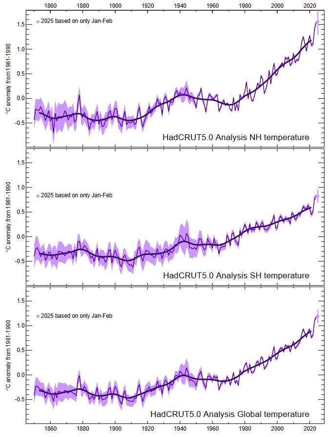
Figure 8.1 Global average surface temperature anomalies 1850 2025. Top: Northern hemisphere. Middle: Southern hemisphere. Bottom: Global average. Source: UK Hadley Centre https://crudata.uea.ac.uk/cru/data/temperature/HadCRUT5.0Analysis.pdf

The causes of the early 20th century warming are discussed by Hegerl et al. (2017; 2019). The atmospheric CO2 concentration increased from 298 ppm in 1905 to 310 ppm in 1941, implying that CO2 had little impact. Volcanic activity during this period was very low, and solar forcing is uncertain. Yet Hegerl et al. (2017) somehow inferred that 40-54 percent of this warming could be attributed to external forcing, with the rest associated with internal variability. Bronniman et al. (2024) focused on the causes of the cooling in the first decade of the 20th century in the Southern Hemisphere. They found that the cooling was related to a La-Niña-like pattern in the Pacific, a cold tropical and subtropical South Atlantic, a cold extratropical South Pacific, and cool southern midlatitude land areas. The Southern Annular Mode was positive, with a strengthened Amundsen–Bellingshausen seas low, although the spread of the data products is considerable.

The warming in the 1930’s and subsequent cooling during mid-century was particularly pronounced in the Arctic. Bokuchava and Semenov (2021) find that these variations were most likely caused by a combined effect of long-term natural climate variations in the North Atlantic and North Pacific with a contribution of the natural radiative forcing related to the reduced volcanic activity and variations of solar activity, as well as growing greenhouse gases concentrations. Tokinaga et al. (2017) showed that the combined effect of internally generated Pacific and Atlantic interdecadal variability intensified Arctic warming in the early 20th century. The synchronized Pacific-Atlantic warming drastically alters planetaryscale circulations over the Northern Hemisphere; these same circulation patterns have a global influence.

The cooling period between 1945 and 1976 has been referred to as the “grand hiatus.” Numerous causes have been hypothesized: natural internal variability from fluctuations associated with the Pacific Decadal Oscillation and Atlantic Multidecadal Oscillation; cooling from increased emissions of aerosols from industrial activities; increased heat uptake in the Atlantic, Southern and Equatorial Pacific Oceans. Thompson et al. (2010) find that that the hemispheric differences in temperature trends in the middle of the twentieth century stem largely from a rapid drop in Northern Hemisphere sea surface temperatures of about 0.3 °C between about 1968 and 1972.

The Great Pacific Climate Shift of 1976-1977 was a notable climatic event characterized by an abrupt change in the North Pacific Ocean's atmosphere-ocean system that interacted with global climate patterns. This shift is closely associated with the Pacific Decadal Oscillation (PDO) that oscillates between warm and cool phases over decades. The 1976 shift marked a transition from a predominantly negative (cool) PDO phase (1947–1976) to a positive (warm) phase (1977 through 2000), with significant implications for global and regional climate patterns, including the frequencies of El Nino and La Nina events. The Great Pacific Climate Shift coincided with the beginning of a period of accelerated global warming. When the Great Pacific Climate Shift is accounted for in climate attribution analyses since 1950, 40 percent or more of the warming in the second half of the 20th century is attributed to natural internal variability (McLean et al., 2009; Tung and Zhou, 2013; Chylek et al., 2016; Scafetta, 2021).

8.3.2

Optimal fingerprinting

Optimal fingerprinting is a statistical technique introduced by Allen and Tett (1999) that compares observed climate data to climate model simulations to identify patterns (or "fingerprints") associated with human or natural forcing. It involves taking a vector of observed climate changes, such as warming rates inlocationsaroundtheworld,anddecomposingtheminto aweightedsumof“signals”,whichareanalogues to the observations generated by climate models with different types of forcings. The weights are chosen using a regression method called Total Least Squares (TLS). The analysis commonly uses just two signals, one generated by models using only anthropogenic forcings and one using only natural forcings. If the estimated weighting coefficient attached to a signal is significantly different from zero, then that signal is said to be “detected”. If it is close to 1.0, then the model generating the signal is said to be consistent with observations. If it is less than 1.0, then the model signal for that forcing is too strong and needs to be scaled down,andvice-versa.Boththeobserveddataandthesignalsareweightedusingamodel-generatedestimate of patterns of randomness in the climate system so as, in principle, to put maximum weight on regions where natural variability is minimized.

Optimal fingerprinting is the primary tool for attribution in the research literature. While it has been widely used and prominently featured by the IPCC since 2001, there is very little literature examining the statistical properties of the results it generates. One of its inherent weaknesses is that results depend on assumptions about the accuracy of climate models, especially regarding their representation of natural variability (IPCC AR5 Ch 10.2.3).

A series of papers by McKitrick (McKitrick 2021, 2022, 2023, 2025) has challenged the optimal fingerprinting method, arguing that it is inherently unreliable and that practices adopted from econometrics can provide more valid results. Statistical theory requires that for regression models to yield unbiased coefficients, a set of assumptions called the Gauss-Markov conditions must hold. McKitrick (2021) argued that the Allen and Tett (1999) methodology violates the Gauss-Markov conditions, leading to potentially biased and inconsistent fingerprinting coefficients, undermining the reliability of the method. Chen et al. (2023) confirmed this analysis, although they argued that the method could yield valid results under very stringent assumptions.McKitrick(2022)and(2023)raisedafurtherconcernthatclimatescientists virtuallyaloneamong scientific disciplines have used TLS to estimate anthropogenic greenhouse gas signal coefficients, despite its tendency to be unstable unless some strong assumptions hold that in practice are unlikely to be true.

Under conditions that easily arise in optimal fingerprinting, TLS estimates have a large positive bias. Thus, any study that used TLS for optimal fingerprinting without verifying its applicability in the specific data context has likely overstated the attribution

McKitrick (2025) presented an empirical example comparing the results of conventional optimal fingerprinting against methods drawn from mainstream econometrics that are known to be valid for the specific application of signal detection. While the IPCC optimal fingerprinting method yields an anthropogenic signal coefficient close to 1.0 on a global temperature data set spanning 1900 to 2010, the consistent method yields a coefficient around 0.4, which rises to about 0.65 on data spanning 1980 to 2010, implying the modelresponse to greenhouse gases needs to be scaled down by about half to optimally match observations. The natural forcing signal coefficient, by contrast, is between 2.0 and 4.0, implying the climate model signals of natural forcing need to be scaled up two-to four-fold to match observed climate change. The fingerprinting coefficients estimated in McKitrick (2025), when used to scale the average sensitivity of the climate models used to generate the forcing signals in his data set, imply a Transient Climate Sensitivity of 1.4°C, which is consistent with the estimate by Lewis (2023) using a different estimation method and multiple independent data sets.

Thesefindings indicatethat thebasis on which theoptimalfingerprinting method has long beenviewed as reliable is not valid. Re-examining previous results individually would be required to determine which findings are statistically robust

8.3.3 Time series methods

The IPCC (AR5 WGI 10.2.2) drew attention to alternative approaches of assessing causality that emerged from the time series econometrics literature. These have the advantage of not depending on assumptions about the accuracy of climate models, but the disadvantage that they depend on difficult-totest assumptions about the data generating process underlying climate and forcing data. The methods, now referred to as climate econometrics, use the tools of unit root testing, Granger causality and cointegration analysis, all of which are familiar in economics and finance and which are slowly being adopted in climate science. Time series analysis methods hold out the possibility of determining whether anthropogenic or natural forcings are the primary drivers of climate change without requiring the use of climate models, although key questions remain unsettled (e.g. Dergiades et al., 2016, Balcombe et al., 2019, Dagsvik et al., 2020, Razzak, 2022, Dagsvik and Moen, 2023).

“Granger causality” modeling is a tool for determining directions of influence in data series that move together. It is a statistical, not a physical, concept. If knowing the currentvalue of one variable significantly improves the forecast accuracy of another variable, we can infer a causal connection exists; this is called Granger causality. The modeling tools, called vector autoregression, measure direct impulse-response patterns and feedbacks. An application to the well-known Vostok ice core data revealed an error in Al Gore’s documentary An Inconvenient Truth. Gore showed the data and drew attention to the coherence of temperature and CO2 changes over a 440,000 year span, which he asserted was due to CO2 driving temperature changes. But temperature changes can also affect atmospheric CO2 levels. Davidson et al. (2015) examined the series and found that temperature Granger causes CO2 but not the reverse. In other words on the time scales represented in the Vostok data, the coherence in the series is primarily due to the influence of temperature on CO2 levels, not the feedback of CO2 levels on temperature.

In summary, the primary statistical methods for attributing causation in climate data are optimal fingerprinting and time series analysis. Applications of the Allen and Tett (1999) optimal fingerprinting method dominate the attribution literature and have underpinned past IPCC conclusions, but results depend on the accuracy of climate models and the method has recently been criticized as inherently biased. Time

series methods do not depend on climate models but require assumptions of their own and have generated results that have thus far not converged on a consensus.

8.4 Declining planetary albedo and recent record warmth

A sharp recent increase in global average temperatures has raised the question of short-term drivers of climate. One such candidate is the fraction of absorbed solar radiation which has also increased abruptly in recent years. The question is whether the change is an internal feedback to warming caused by greenhouse gases, or whether something else increased the fraction of absorbed radiation which then caused the recent warming.

The planetary albedo is the fraction of incoming solar radiation that is reflected back into space rather than being absorbed by the planet. Highly reflective surfaces like cloud tops and snow and ice are most important in this regard. The Earth's albedo is approximately 30 percent, meaning almost a third of the sunlight that reaches Earth is directly reflected back to space. A lower albedo implies more solar energy is absorbed by the planet to be then re-radiated as heat. Hence, other things being equal, a decline in planetary albedo is associated with a warming of the Earth.

Arguably the most striking change in the Earth’s climate system during the 21st century is a significant reduction in planetary albedo since 2015, which has coincided with at least two years of record global warmth. Figure 8.2 shows the planetary albedo variations since 2000, when there are good satellite observations. The 0.5 percent reduction in planetary albedo since 2015 corresponds to an increase of 1.7 W/m2 in absorbed solar radiation averaged over the planet (Hansen and Karecha, 2025). For comparison, Forster et al. (2024) estimate the current forcing from the increase in atmospheric CO2compared to preindustrial times to be 2.33 W/m2

Looking back prior to 2000 with less adequate data, Goessling et al. (2025) assessed that the planetary albedo was relatively low around the 1940’s and 50’s before rising industrial aerosol precursor emissions increased the albedo until the 1980’s. The strongest planetary albedo excursions were high-albedo episodes caused by volcanic eruptions, such as after the Mount Pinatubo eruption in 1991. Although uncertain, the 2023 planetary albedo minimum might have been the lowest since at least 1940.

Changes in surface characteristics cannot explain this decrease in planetary albedo since 2015:

• Arctic sea ice extent has declined by about 5 percent since 1980 (https://nsidc.org/data/seaice_index/images/s_plot_hires.png), although following 2007 there has been a pause in the Arctic sea ice decline (England et al., 2025)

• Regarding Antarctic sea ice, the IPCC AR6 concludes that “There has been no significant trend in Antarctic sea ice area from 1979 to 2020 due to regionally opposing trends and large internal variability.” (Summary for Policymakers, A.1.5)

• Northern hemispheric annual snow cover has been slowly declining since 1967, with barely significant trends. The data show the Northern Hemisphere has snowier winters, accompanied by more rapid melt in spring and summer, see http://climate.rutgers.edu/snowcover/ and Section 5.6

• Global greening (Chapter 2) is contributing to the decrease in planetary albedo, as forests have a lower albedo than open lands or snow. However, there is some evidence that forests increase cloud cover (high reflectivity), which counteracts the direct albedo decrease associated with increasing forested area.

Figure 8.2. Earth’s albedo (reflectivity, in percent), with seasonality removed. From Hansen and Karecha (2025)

Changes in surface reflectivity are contributing to a small, slow decline in planetary albedo. However, these changes cannotexplain the sharp decline in planetary albedo beginning in 2015. Further, any changes in surface albedo are effectively damped by about a factor of three on average, primarily due to cloud masking (Loeb et al. 2019). Surface albedo changes have thus contributed only weakly to the recent planetary albedo decline, particularly when averaged annually and globally. This leaves the most likely explanation for the sharp albedo decline as changes in atmospheric aerosols and/or clouds.

Aerosols are smallparticles in theatmosphere that reflect sunlight and can interact withcloud processes to make the clouds more reflective. Aerosols have both natural origins (e.g dust from soils, wildfires) as well as human origins from combustion (including fossil fuels). Regions that are greening and/or have an increase in rainfall might produce less dust. For anthropogenic aerosols, new ship fuel regulations aimed at reducing sulfur emissions were implemented in three phases, in 2010, 2015 and 2020 Sulfate particles reflect solar radiation, so cleaner air means less solar radiation is reflected, which contributes to surface warming. Indirect effects of sulfate aerosols include increasing the reflectivity of low-level clouds in the subtropics. There is controversy surrounding the importance of this change in sulfate emissions to the Earth’s radiation balance (Hodnebrog et al., 2024; Yuan et al., 2024), but the restriction of this effect to major shipping routes suggests a small global impact (Schmidt, 2024).

Changes in clouds are the primary candidate to explain the decline in global albedo since 2015. Two recent papers (Loeb et al., 2024; Goessling et al 2024) have addressed recent variations in cloud properties. By considering satellite and reanalysis data, Loeb et al. found that decreases in low- and mid-level clouds since 2015 are the primary reason for decreasing planetary albedo in the Northern hemisphere, whereas in the Southern hemisphere the decrease in planetary albedo is primarily due to decreases in mid-level clouds across all latitude zones. Goessling et al. (2024) found that cloud anomalies were mainly due to reduced low-level clouds. Regions with coherent low-level cloud reductions over the past decade include the warm pool region around the Maritime Continent and the northern extratropical western Pacific, as well as large parts of the Atlantic and adjacent land regions. The reduction of global cloud cover identified in these analyses since 2015 is 1-2 percent.

The issue then becomes the cause of the change in cloud cover. Two explanations have been posited for the declining cloud cover over the past decade:

• Natural climate variability

• Changes in low cloud cover associated with warming sea surface temperatures, implying an emerging positive feedback to climate change (Hansen and Karecha, 2025)

It is not easy to justify a new positive low cloud feedback that began emerging in 2015 since there is no obvious feedback trigger starting at that time However, there are numerous natural climate signals during this period that are associated with atmospheric circulation changes that can influence the distribution of clouds:

• The 2014-2016 was one of the strongest El Niño events on record

• A cold anomaly beginning in 2015 in the subpolar gyre of the North Atlantic reflects a shift in the ocean circulation pattern associated with decadal variability in the Atlantic (Frajka-Williams et al., 2017; Arthun et al. 2021).

• The Pacific Decadal Oscillation positive index peaked in 2016, then declined and has been in negative territory since late 2019

• Eruption of the submarine Hunga-Tonga volcano in 2022

Interannual cloud anomalies associated with the El Niño Southern Oscillation (ENSO) have a significant global signal and strong regional signals, especially over the tropical Indian and Pacific Oceans.

The Hunga Tonga eruption is remarkable in its coincidence with the exceptionally low value of planetary albedo in 2023. Goessling et al. (2024) found that the cloud perturbations in 2023 showed a different pattern from the overall pattern since 2015, with reduced cloud cover being most pronounced in the northern hemisphere and tropics. Regional reductions in cloud cover were most pronounced over the eastern Indian Ocean, over South America and extending over the eastern Pacific, as well as over northern North America, in the Southern Ocean around 60S, in the subtropical and eastern North Atlantic, and in parts of the North Pacific.

The Hunga Tonga eruption was unusual in that it injected large amounts of water vapor into the stratosphere in addition to sulfate particles. Early publications focused on the impacts to stratospheric circulations and the direct radiative impact. In 2025, papers are emerging that examine the indirect effects of Hunga Tonga on surface climate using ensemble simulations from earth system models (Bednarz et al., 2025; Kuchar et al., 2025). These papers found statistically significant impacts on regional climates that were driven by circulation changes from couplings between the stratosphere and troposphere. These papers indicate the complex interactions between volcanic activity and climate dynamics. More research is needed to untangle any impacts of the Hunga Tonga eruption on the planetary albedo.

In summary, the decline in planetary albedo and the concurrent decline in cloudiness have emphasized the importance of clouds and their variations to global climate variability and change. A change of 1- 2 percent in global cloud cover has a greater radiative impact on the climate than the direct radiative effect of doubling CO2. While it is difficult to untangle causes of the recent trend, the competing explanations for the cause of the declining cloud cover have substantial implications for assessing the Equilibrium Climate Sensitivity and for the attribution of the recent warming. An additional 10 years of data should help clarify whether this is a strong positive cloud feedback associated with warming or a temporary fluctuation driven by natural variability

8.5 Attribution of climate impact drivers

The IPCC (Ranasinghe et al. 2021) defines “climate impact drivers” or CIDs as “physical climate system conditions (e.g., means, events, extremes) that affect an element of society or ecosystems.” Hence CIDs are those features of the weather and climate system of primary interest in assessing the impacts of climate change since they potentially affect humans and the natural world. For instance, under the heading “Heatand Cold,” CIDs areidentified as meanair temperature, extreme heat,cold spells and frost. The IPCC

also points out that CIDs are not necessarily harm-related:depending on the system in question they can be detrimental, neutral, beneficial or a combination.

The first columns Table 12.12 in Ranasinghe et al. (2021, p. 1856), reproduced here as Table 8.1, summarize the AR6 assessment of whether a signal of attributable anthropogenic influence has emerged across all major CIDs. One of the themes of this chapter is that attribution methods used by the IPCC tend to overstate the anthropogenic influence and understatetherole of natural variability. Nonetheless astriking feature of that summary table is how few CIDs exhibit an anthropogenic signal sufficient to distinguish them from natural variability.

Out of the 33 weather impact categories listed, an anthropogenic signal is asserted with high confidence in only five, and with medium confidence in a further four. (Note that one of the CIDs is an increase in CO2 levels, and since it is a tautology to attribute this to increased CO2 levels this CID can be ignored.) For the restthe IPCC does notclaim to have detected anthropogenic drivers. Of thefive high confidence assertions, two are for changes in average temperatures (air and ocean) hence are not measures of extreme weather. Further, two of the four medium confidence assertions are related to ocean chemistry and thus are likewise not related to extreme weather. The IPCC does not assert a human influence on many non-temperature weather features such as wind, precipitation, flooding, or drought

Other columns of IPCC Table 12.12 report on whether anthropogenic signals are expected to emerge this century under RCP8.5, the most extreme forcing scenario. We have omitted these columns for several reasons. First, because they refer to whether climate models project detectable signals in the observations, which is a very different question than our concern here: whether a signal has been detected in historical data. Second, as we discuss in Chapter 4, the RCP8.5 scenario is a misleading and implausible high-end storyline, it is not a “base case” or business-as-usual projection. Third, the ensemble of detailed models is acknowledged (Palmer and Stevens 2019) to be “not fit for purpose” in describing regional changes and “unable to represent future conditions at the degree of spatial, temporal, and probabilistic precision with which projections are often provided.” (Nissan et al, 2019). Even with these caveats, we note that the omitted columns in AR6 Table 12.12 show most weather impacts are not expected to exhibit an anthropogenic signal through the end of this century.

As discussed in Chapter 6 natural variability dominates patterns of extreme weather systems and simplistic assertions of trend detection are frequently undermined by regional heterogeneity and trend reversals over time. Table 8.1 makes the related point that it is not currently possible to attribute changes in most extreme weather types to human influences. Taking wind as an example, the IPCC claims that an anthropogenic signalhas notemerged in average wind speeds, severe windstorms, tropical cyclones or sand and dust storms, nor is one expected to emerge this century even under an extreme emissions scenario. The same applies to drought and fire weather.

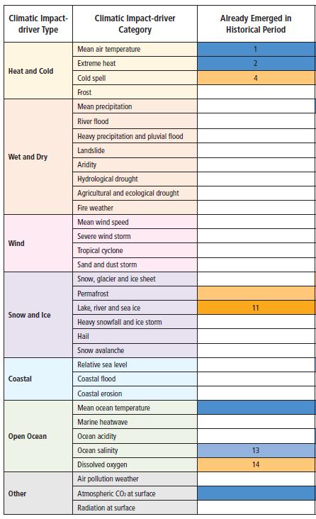
Table 8.1: Reproduction of column 1 of Table 12.12, IPCC AR6 Working Group I report. Emergence of anthropogenic signal in historical period for CIDs shown. White: no signal detected. Blue and orange: change detected (decrease or increase) and confidence level as indicated in color legend. Numbers refer to specific regions and confidence levels: see original Table for notes.

8.6

Extreme event attribution (EEA)

Examining the IPCC’s treatment of extreme weather and climate event attribution more broadly, AR6 provides an ambiguous assessment of the role of anthropogenic warming that differs between its chapters. Chapter 11 of WG1 states (Seneviratne et al., 2021):

Evidence of observed changes in extremes and their attribution to human influence (including greenhouse gas and aerosol emissions and land-use changes) has strengthened since AR5, in particularfor extreme precipitation, droughts, tropical cyclones and compound extremes (including dry/hot events and fire weather). Some recent hot extreme events would have been extremely unlikely to occur without human influence on the climate system.

By contrast, as noted in Section 8.5, Chapter 12 of WG1 (Table12.12) paints a different picture –presumably, the expert judgment of different groups of authors for the two chapters came to different conclusions (Ranasinghe, 2021):

• High confidence in an increase in extreme heat events in tropical regions where observations allow trend estimation and in most regions in the mid-latitudes, medium confidence elsewhere

• Medium confidence in a decrease in extreme cold events in Australia, Africa and most of northern South America where observations allow trend estimation

• No evidence of emergence in the historical period of a change in river floods, heavy precipitation, drought, fire weather, severe windstorms, and tropical cyclones

While the overall issue of detecting changes in extreme weather events and their attribution remains ambiguous, most of the activity in this area relates to the attribution of particular extreme weather events. The most prominent effort is World Weather Attribution (WWA; worldweatherattribution.org), an international research initiative for extreme event attribution that purports to analyze how climate change influences the likelihood and intensity of extreme weather events. Their approach is to use large ensembles ofregionalclimatemodelstocompare aneventintoday’sclimatewithoneinacounterfactualpre-industrial climate without human influences.

WWA has a prominent public presence in linking extreme weather to climate change, with its press releases attracting considerable attention in public and policy discussions. However, WWA’s extensive promotion of non-peer-reviewed findings, its open admission to shaping analyses to serve litigation, and its methodological challenges have sparked controversies, with critics questioning the robustness and impartialityoftheirconclusions (Pielke Jr. 2024).Despitetheseissues,WWA’sworkcontinuestoinfluence climate science and media narratives. Technical criticisms of the approach include a lack of a formal detection process; an implicit assumption that 100 percent of the post-industrial warming is caused by greenhouse gases; and a failure to adequately account for internal climate variability.

Because EEA is relatively new, many basic methodological issues have yet to be settled in the expert literature. An important challenge is the lack of data. Extreme events are by definition rare. Many analyses of extreme event types (including the U.S. National Assessment Reports) only evaluate data since 1950 or 1970. However, as emphasized in Chapter 6, many of theworst extreme weather and climate events in U.S. history occurred in or before the first half of the 20th century, including in the early 19th century. And if paleoclimate reconstructions are considered, it becomes very difficult for an event to pass thresholds of whatis expected fromnatural variability, particularly if a reasonably sized geographic region is considered.

Another challenge is defining the event under study. There is a longstanding literature in statistics and econometrics on the challenge of analyzing data with outliers. The issue arises because a data series establishes a probability distribution defining the expected range of observations. If an outlier is observed it might indicate that the underlying process giving rise to the data distribution has changed (which in the weather context would mean that a climate change has been detected) or that the underlying process has multiple regimes each with a different probability distribution, in which case observing an outlier simply means we were temporarily in a different regime, but the system itself was unchanged. If a time series contains only a single outlier event at the end of the series, it is not possible to determine which model is the correct one (Chen and Liu 1993). For instance, there might be an “ordinary” weather regime that yields a distribution of summer daytime highs in a particular coastal region, and a second “heatwave” regime that kicksinwhenaninlandblockingeventoccurs,whichyieldsatemperaturedistributioncentered15°Chigher than the first one. A day with temperatures 13°C above normal would either be an extreme heat anomaly under the first regime or a somewhat cool event under the second, and we have no way in this case of knowing on statistical grounds which view is correct.

Visser and Petersen (2012) and Sardeshmukh et al. (2015) both point out that different distributions might fit observed data equally well but yield very different implications about the likelihood of a specific weatherevent. Visserand Petersenarguethat, in view ofthe deep uncertainties ofextreme weatheranalysis, drawingaconnectionbetweenindividualeventsandglobalclimatechangeshouldbeavoided.Furthermore, the existence of an outlier at the end of a data series poses the problem that estimates of the event probabilities will be biased whether the outlier is included or excluded (Barlow et al., 2020). Methods to eliminate the bias have not yet been established, leading some experts (e.g. Miralles and Davison 2023) to argue that in settings in which a data series contains a single extreme event at the end, estimation of a return period for the extreme event will be so biased and uncertain that it should be avoided altogether.

We provide a case study of a recent high impact extreme event in the U.S. to illustrate the challenges and ambiguities in attributing the frequency and intensity of extreme weather events to human-caused warming.

8.6.1 Case study – 2021 Western North America heat wave

The 2021 Western North America heat wave was an extreme event that affected much of Western North America in late June 2021. Surface temperature records were set in Portland, OR (116°F; previous record 107°F) and Seattle, WA (108 °F; previous record 103°F) (Mass et al., 2024).

The WWA team generated international headlines with their analysis, which provided the following attribution statements (WWA, 2021; Philip et al., 2022):

• Based on observations and modeling, the occurrence of this heatwave was virtually impossible without human-caused climate change.

• The event is estimated to be about a one in 1000-year event in today’s climate.

• The event would have been at least 150 times rarer without human-induced climate change.

• This heatwave was about 2°C hotter than it would have been if it had occurred at the beginning of the industrial revolution (when global mean temperatures were 1.2°C cooler than today).

But an important counter to the first claim is that other researchers concluded from historical weather data that while a heat wave of the magnitude observed was indeed virtually impossible without anthropogenic climate change, it was also virtually impossible with climate change. Bercos-Hickey (2022) noted “these temperatures were virtually impossible under any previously experienced meteorological conditions, with or without global warming.” McKinnon and Simpson (2022) stated “the most likely explanation remains that the weather event itself was ‘bad luck.’” The 2023 Oregon Climate Assessment (Fleischman, 2023) concluded that the heat dome would have formed even without climate change and “There is no evidence that the highly unusual combination of weather features that drove the heat dome

were made more likely by climate change, and climate models do not project an increase in the frequency of high-pressure ridges over the Pacific Northwest” (Fleischman, 2023, p. 49).

Mass et al. (2024) summarizes the proximate sequence of compound events leading to the heat wave. There was a record-breaking mid-tropospheric ridge over the Pacific Northwest, forced by a tropical disturbance in the western Pacific. This produced record-breaking mid-tropospheric temperatures, strong subsidence in the lower atmosphere, low-level easterly flow that produced downslope warming on regional terrain and the removalof cooler marine air, and an approaching low-level trough that enhanced downslope flow. The eventoccurred ata time of maximum solar insolation, and drier-than-normal soilmoisture. Using a storyline approach, Mass et al. assessed that there was no trend in drought and dry soils in the Pacific Northwest; there is no evidence of global warming producing stronger ridges of high pressure, and no observed trend in heat waves or record temperatures in the region. They concluded that although anthropogenic warming might have contributed as much as 2°F to the magnitude of the event, there is little evidence of further amplification of the event from increasing greenhouse gases.

Bercos-Hickey et al. (2022) conducted a statistical analysis of a model-based attribution study of this heat wave Because the event is a far outlier and far above the bounds of Generalized Extreme Value distributions fitted from historical data, they concluded that estimates of return times, quantitative changes in event magnitude and frequency, and probability of the extreme temperatures such as provided by the WWA are not accurate and should be interpreted as having low confidence. They found that hindcast attribution methods using an ensemble of regional climate models, combined with Pearl (2009) causal inferences, can provide limited and conditional information about the magnitude of the human influence on this heatwave - they provided a more highly constrained estimate that human activities caused a ∼1.4°F–1.8°F increase in the daily maximum temperatures.

Zeder et al. (2023)alsoconcludedthatthemethodsemployedbyPhilip et al. (2022,theWWAanalysis) tend to overstate the rarity of extreme heat waves, leading to a biased perception of the effect of climate change on the heatwave event: “The tendency to overestimate the return period of observed extreme heatwave events may fuel the impression that seemingly impossible heatwave extremes are currently clustering at an unprecedented rate.”

The 2021 Western North America heatwave was a rare and unprecedented compound weather event that broke century-old temperature records by as much as 9°F. While the WWA team received worldwide publicity for their rapid attribution claims blaming anthropogenic climate change, subsequent peerreviewed analyses showed that the event was caused by rare meteorological conditions that were not made more probable by global warming.

References

Allen, M. R., & Tett, S. F. B. (1999). Checking for model consistency in optimal fingerprinting. Climate Dynamics, 15(6), 419–434. https://doi.org/10.1007/s003820050291

AR4: Intergovernmental Panel on Climate Change Fourth Assessment Report (2021) Working Group I Contribution. www.ipcc.ch.

AR5: Intergovernmental Panel on Climate Change Fifth Assessment Report (2021) Working Group I Contribution. www.ipcc.ch.

AR6: Intergovernmental Panel on Climate Change Sixth Assessment Report (2021) Working Group I Contribution. www.ipcc.ch.

Arthun, M, RCJ Willis, HL Johnson, L Chafik, HR Langehaug (2021) Mechanisms of Decadal North Atlantic Climate Variability and Implications for the Recent Cold Anomaly. Journal of Climate, Vol 34

Balcombe,Kevin,IainFraserandAbhijitSharma(2019)Isradiativeforcingcointegratedwithtemperature? A further examination using a structural time series approach.” Management of Environmental Quality 30(5) DOI 10.1108/MEQ-12-2018-021.

Barlow, Anna Maria, Chris Sherlock and Jonathan Tawn (2020) Inference for Extreme Values Under Threshold-Based Stopping Rules. Journal of the Royal Statistical Society Series C August 2020, Pages 765–789, https://doi.org/10.1111/rssc.12420

Bednarz, EW, AH Butler, X Wang, Z Zhou, W Yu, G Stenchikov, M Toohey, Y Zhu (2025) Indirect climate impacts of the Hunga eruption. Preprint, https://doi.org/10.5194/egusphere-2025-1970

Bercos-Hickey, E., et al. (2022). Anthropogenic contributions to the 2021 Pacific Northwest heatwave. Geophysical Research Letters, 49(23), e2022GL099396. https://doi.org/10.1029/2022GL099396

Bokuchava, DD and VV Semenov (2021) Mechanisms of the early 20th century warming in the Arctic. Earth-Science Reviews, 222, 103820

Chatzistergos, T., Krivova, N. A., & Yeo, K. L. (2023). Long-term changes in solar activity and irradiance. Journal of Atmospheric and Solar-Terrestrial Physics, 252, 106150. https://doi.org/10.1016/j.jastp.2023.106150

Chen, C., & Liu, L.-M. (1993). Joint estimation of model parameters and outlier effects in time series. Journal of the American Statistical Association, 88(421), 284–297. http://www.jstor.org/stable/2290724

Chen, H, SX Chen and M Mu (2023) A statistical review on the optimal fingerprinting approach in climate change studies. Climate Dynamics 62:1439-1446 https://link.springer.com/article/10.1007/s00382023-06975-5

Chylek, P., et al. (2016). The role of Atlantic Multi-Decadal Oscillation in the global mean temperature variability. Climate Dynamics, 47(9–10), 3271–3279. https://doi.org/10.1007/s00382-016-3025-7

Connolly, R., et al. (2021). How much has the sun influenced Northern Hemisphere temperature trends? An ongoing debate. Research in Astronomy and Astrophysics, 21(6), 131. https://doi.org/10.1088/1674-4527/21/6/131

Cramer, W., et al. (2014). Detection and attribution of observed impacts. In C. B. Field et al. (Eds.), Climate Change 2014: Impacts, Adaptation, and Vulnerability. Part A: Global and Sectoral Aspects (pp. 979–1037). Cambridge University Press.

Dagsvik, JK SH Moen (2023) To what extent are temperature levels changing due to greenhouse gas emissions? Statistics Norway Discussion Paper 1007 September 2023

Dagsvik, JK, M Fortuna and SH Moen (2020) How Does Temperature Vary Over Time?: Evidence on the Stationary and Fractal Nature of Temperature Fluctuations. Journal of the Royal Statistical Society Series A: Statistics in Society, Volume 183, Issue 3, June 2020, Pages 883–908, https://doi.org/10.1111/rssa.12557

Davidson, James E.H., David B. Stephenson and Alemtsehai A. Turasie (2015) Time series modeling of paleoclimate data Environmetrics 27(1) https://onlinelibrary.wiley.com/doi/abs/10.1002/env.2373

Dergiades, T., R.K. Kaufmann and T. Panagiotidis (2016). Long-run changes in radiative forcing and surface temperature: The effect of human activity over the lastfive centuries. Journal of Environmental Economics and Management 76:67 85. https://www.sciencedirect.com/science/article/abs/pii/S0095069615000911

England, Mark, Lorenzo M Polvani, James A Screen, et al (2025). Surprising, but not unexpected, multidecadal pause in Arctic sea ice loss. ESS Open Archive. March 29, 2025.

Fleishman, E., editor. (2023). Sixth Oregon Climate Assessment. Oregon Climate Change Research Institute, Oregon State University, Corvallis, Oregon. https://blogs.oregonstate.edu/occri/oregonclimate-assessments

Forster et al. (2024) “Indicators of Global Climate Change 2024: annual update of key indicators of the state of the climate system and human influence” Earth System Science Data 17(6) https://doi.org/10.5194/essd-17-2641-2025

Frajka-Williams, E, C Beaulieu, Aurelie Duchez (2017) Emerging negative Atlantic Multidecadal Oscillation index in spite of warm subtropics. Scientific Reports, 7:11224

Goessling, Helge F. Thomas Rackow and Thomas Jung (2024) Recent global temperature surge intensified by record-low planetary albedo Science Vol 387, Issue 6729 pp. 68-73 https://www.science.org/doi/abs/10.1126/science.adq7280

Gulev, S. K., et al. (2021). Changing state of the climate system. In V. Masson-Delmotte et al. (Eds.), Climate Change 2021: The Physical Science Basis. Contribution of Working Group I to the Sixth Assessment Report of the Intergovernmental Panel on Climate Change (pp. 287–422). Geneva: Intergovernmental Panel on Climate Change.

Hansen J and P Karecha (2025) Large cloud feedback confirms high sensitivity. https://www.columbia.edu/~jeh1/mailings/2025/CloudFeedback.13May2025.pdf

Hegerl, G. C., et al. (2007). Understanding and attributing climate change. In S. Solomon et al. (Eds.), Climate Change 2007: The Physical Science Basis. Contribution of Working Group I to the Fourth Assessment Report of the Intergovernmental Panel on Climate Change (pp. 663–745). Cambridge University Press.

Hegerl, GC, S Bronniman, A Schurer et al. (2017) Early 20th century warming: Anomalies, causes and consequences. WIRES Climate Change, DOI: 10.1002/wcc.522

Hegerl, GC, S Bronniman, T Cowan (2019) Causes of climate change over the historical record. Environmental Research Letters, 14, 123006

Hodnebrog, Ø et al. (2024), Recent reductions in aerosol emissions have increased Earth’s energy imbalance. Communications Earth and Environment 5, 166 (2024). doi:10.1038/s43247-024-01324-8

Houghton, J. T., et al. (Eds.). (2001). Climate Change 2001: The Scientific Basis. Contribution of Working Group I to the Third Assessment Report of the Intergovernmental Panel on Climate Change (pp. 1–881). Cambridge University Press.

https://mailchi.mp/caa/large-cloud-feedback-confirms-high-climate-sensitivity

Kravtsov, S., Westgate, A., & Gavrilov, A. (2024). Global-scale multidecadal variability in climate models and observations, part II: The stadium wave. Climate Dynamics, 62, 10281–10306. https://doi.org/10.1007/s00382-024-07451-4

Kuchar, A., Sukhodolov, T., Chiodo, G., Jörimann, A., Kult-Herdin, J., Rozanov, E., and Rieder, H. H. (2025): Modulation of the northern polar vortex by the Hunga Tonga–Hunga Ha'apai eruption and the associated surface response, Atmospheric Chemistry and Physics, 25, 3623–3634, https://doi.org/10.5194/acp-25-3623-2025

Lewis, Nicholas (2023) “Objectively Combining Climate Sensitivity Evidence,” Climate Dynamics 61, no. 9–10 (2023): 3155–3163, https://doi.org/10.1007/s00382-022-06398-8 .

Lockwood, M. (2012). Solar influence on global and regional climates. Surveys in Geophysics, 33(3–4), 503–534. https://doi.org/10.1007/s10712-012-9181-3

Loeb, N. G. et al. (2019) Decomposing Shortwave Top-of-Atmosphere and Surface Radiative Flux Variations in Terms of Surface and Atmospheric Contributions. Journal of Climate 32(16), 50035019 (2019). doi:10.1175/JCLI-D-18-0826.1

Loeb, N., S-H Ham, RP Allen, TJ Thorsen, B Meyssignac, S Kato, GC Johnson, JL Lyman (2024)

Observational Assessment of Changes in Earth’s Energy Budget since 2000. Surveys in Geophysics, 45, 1757-1783

Mass, C., et al. (2024). The Pacific Northwest heat wave of 25–30 June 2021: Synoptic/mesoscale conditions and climate perspective. Weather and Forecasting, 39(2), 275–291. https://doi.org/10.1175/WAF-D-23-0154.1

Matthes, K., et al. (2017). Solar forcing for CMIP6 (v3.2). Geoscientific Model Development, 10(6), 2247–2302. https://doi.org/10.5194/gmd-10-2247-2017

McKinnon, K. and I. Simpson (2022) How Unexpected Was the 2021 Pacific Northwest Heatwave? Geophysical Research Letters, 49, e2022GL100380. https://doi.org/10.1029/2022GL100380

McKinnon, K. and I. Simpson (2022) How Unexpected Was the 2021 Pacific Northwest Heatwave? Geophysical Research Letters, 49, e2022GL100380. https://doi.org/10.1029/2022GL100380

McKitrick, R. (2021). Checking for model consistency in optimal fingerprinting: A comment. Climate Dynamics, 58(1–2), 405–411. https://doi.org/10.1007/s00382-021-05913-7

McKitrick, R. (2023). Total least squares bias in climate fingerprinting regressions with heterogeneous noise variances and correlated explanatory variables. Environmetrics, 35(2), e2835. https://doi.org/10.1002/env.2835

McKitrick, Ross R (2022) On the choice of TLS versus OLS in climate signal detection regression Climate Dynamics 10.1007/s00382-022-06315-z

McKitrick, Ross R (2025) Consistent Climate Fingerprinting. Climate Dynamics forthcoming preprint available at www.rossmckitrick.com

McLean, J.D., C. R. de Freitas, and R. M. Carter, (2009) “Influence of the Southern Oscillation on Tropospheric Temperature,” Journal of Geophysical Research: Atmospheres 114, no. D14 (July 23, 2009): D14104, https://doi.org/10.1029/2008JD011637.

Miralles, Ophélia and Anthony Davison (2023) Timing and spatial selection bias in rapid extreme event attribution. Weather and Climate Extremes 41 100584 https://doi.org/10.1016/j.wace.2023.100584

Myhre, G., D. Shindell, F.-M. Bréon, et al (2013): Anthropogenic and Natural Radiative Forcing. In: Climate Change 2013: The Physical Science Basis. Contribution of Working Group I to the Fifth Assessment Report of the Intergovernmental Panel on Climate Change [Stocker, T.F., et al. (eds.)]. Cambridge University Press, Cambridge, United Kingdom and New York, NY, USA.

Nissan, Hannah, Lisa Goddard, Erin Coughlan de Perez, et al. (2019) On the use and misuse of climate change projections in international development. Wires Climate Change 14 March 2019 https://doi.org/10.1002/wcc.579

Palmer, Tim N and Bjorn Stevens (2019) The scientific challenge of understanding and estimating climate change. Proceedings of the National Academy of Sciences 116 (49) 24390-24395 https://doi.org/10.1073/pnas.1906691116

Pearl, J. (2009). Causality. Cambridge University Press.

Philip, S. Y., et al. (2022). Rapid attribution analysis of the extraordinary heatwave on the Pacific coast of the U.S. and Canada June 2021. Earth System Dynamics, 13(4), 1689–1713. https://doi.org/10.5194/esd-13-1689-2022

Pielke Jr., Roger (2024) Weather Attribution Alchemy. Substack essay https://rogerpielkejr.substack.com/p/weather-attribution-alchemy

Ranasinghe, R., Ruane, A. C., Vautard, R., Arnell, N., Coppola, E., Cruz, F. A., ... Zaaboul, R. (2021). Chapter 12: Climate change information for regional impact and for risk assessment. In V. MassonDelmotte et al. (Eds.), Climate Change 2021: The Physical Science Basis. Contribution of Working Group I to the Sixth Assessment Report of the Intergovernmental Panel on Climate Change (pp. 1767–1926). Cambridge University Press. https://doi.org/10.1017/9781009157896.014

100

Razzak, Weshah A. (2022). "The Econometrics of Global Warming," Journal of Economics and Econometrics, vol. 65(2), pages 13-47.

Sardeshmukh, P. D., Compo, G. P., & Penland, C. (2015). Need for caution in interpreting extreme weather statistics. Journal of Climate, 28(23), 9166–9187. https://doi.org/10.1175/JCLI-D-15-0020.1

Scafetta, N. (2013). Discussion on climate oscillations: CMIP5 general circulation models versus a semiempirical harmonic model based on astronomical cycles. Earth-Science Reviews, 126, 321

Scaffeta, Nicola (2021) “Reconstruction of the Interannual to Millennial Scale Patterns of the Global Surface Temperature,” Atmosphere 12, no. 2: 147, https://doi.org/10.3390/atmos12020147

Schmidt, G. (2024) Climate models can’t explain 2023’s huge heat anomaly we could be in uncharted territory. Nature 627, 467. https://www.nature.com/articles/d41586-024-00816-z

Schmutz, Werner K. (2021) “Changes in the Total Solar Irradiance and Climatic Effects,” Journal of Space Weather and Space Climate 11: 40, https://doi.org/10.1051/swsc/2021016.

Seneviratne, S. et al. (2021) “Chapter 11: Weather and Climate Extreme Events in a Changing Climate.” In Climate Change 2021: The Physical Science Basis. Contribution of Working Group I to the Sixth Assessment Report of the Intergovernmental Panel on Climate Change, edited by V. MassonDelmotte, P. Zhai, A. Pirani, S.L. Connors, C. Péan, S. Berger, N. Caud, et al., 1513–1766. Cambridge: Cambridge University Press, 2021. https://doi.org/10.1017/9781009157896.013.

Solanki, S.K. et al. (2004), “Unusual Activity of the Sun during Recent Decades Compared to the Previous 11,000 Years,” Nature 431, no. 7012 (October 28, 2004): 1084–1087, https://doi.org/10.1038/nature02995.

Stefani, Frank (2021) “Solar and Anthropogenic Influences on Climate: Regression Analysis and Tentative Predictions,” Climate 9, no. 11 (November 3, 2021): 163, https://doi.org/10.3390/cli9110163.

Thompson, DJW, JM Wallace, JJ Kennedy, PD Jones (2010) An abrupt drop in Northern Hemisphere Sea Surface Temperature around 1970. Nature, 467, 444-447

Tokinaga, H, SP Xie, and H Mukougawa (2017) Early 20th century Arctic warming intensified by Pacific and Atlantic multidecadal variability. Proceedings of the National Academy of Sciences, 114, 6227-6233 https://www.pnas.org/doi/abs/10.1073/pnas.1615880114

Tung, Ka-Kit and Jiansong Zhou (2013) “Using Data to Attribute Episodes of Warming and Cooling in Instrumental Records,” Proceedings of the National Academy of Sciences 110, no. 6 (January 23, 2013): 2058–2063, https://doi.org/10.1073/pnas.1212471110.

Usoskin, I.G., S. K. Solanki, and G. A. Kovaltsov (2007) “Grand Minima and Maxima of Solar Activity: New Observational Constraints,” Astronomy & Astrophysics 471, no. 1 (June 6, 2007): 301–309, https://doi.org/10.1051/0004-6361:20077704

Velasco Herrera, V.M., B. Mendoza, and G. Velasco Herrera (2015) “Reconstruction and Prediction of the Total Solar Irradiance: From the Medieval Warm Period to the 21st Century,” New Astronomy 34 (January 2015): 221–233, https://doi.org/10.1016/j.newast.2014.07.009.

Visser, H. and A.C. Petersen (2012) Inferences on weather extremes and weather-related disasters: a review of statistical methods Climates of the Past 8, 265–286 https://cp.copernicus.org/articles/8/265/2012/cp-8-265-2012.pdf

World Weather Attribution (2021) “Western North American Extreme Heat Virtually Impossible without Human-Caused Climate Change.” July 7, 2021. https://www.worldweatherattribution.org/westernnorth-american-extreme-heat-virtually-impossible-without-human-caused-climate-change/.

Yuan, et al. (2024) Abrupt reduction in shipping emission as an inadvertent geoengineering termination shock produces substantial radiative warming. Communications Earth and Environment 5, 281 (2024). doi:10.1038/s43247-024-01442-3

Zeder, J., Sippel, S., Pasche, O. C., Engelke, S., & Fischer, E. M. (2023). The effect of a short observational record on the statistics of temperature extremes. Geophysical Research Letters, 50, e2023GL104090. https://doi.org/10.1029/2023GL104090

PART III: IMPACTS ON ECOSYSTEMS AND SOCIETY

9 CLIMATE CHANGE AND U.S. AGRICULTURE

Chapter summary

There has been abundant evidence going back decades that rising CO2 levels benefit plants, including agriculturalcrops, and that CO2-induced warming will be a netbenefit to U.S. agriculture. The increase in ambient CO2 has also boosted productivity of all major U.S. crop types. There is reason to conclude that on balance climate change has been and will continue to be neutral or beneficial for most U.S. agriculture

9.1 Econometric analyses

Econometric analyses of the effects of climate change on agriculture have sought to integrate information about long term crop yield changes in response to temperature and precipitation changes under assumptions about adaptive behavior by farmers. One method focuses on variations in agricultural land values. The rationale is that if climate change is a long-term net benefit for agriculture it should be capitalized into higher market values for agricultural land, and vice versa. While individual crops might benefit from, or be harmed by, climate change, once the adaptative responses of farmers are considered the value of farmland represents an index of whether the changes are expected to be beneficial or not. Mendelsohn et al. (1994) examined the relationship between historical climatic variations on agricultural land values and concluded global warming would be slightly beneficial to American agriculture.

The Mendelsohn et al. method, called Ricardian analysis after David Ricardo, the 19th century British economist who pioneered the study of land values, attracted subsequent criticism from authors who argued it failed to account for differences in land values attributable to fixed locational characteristics like soil quality, and non-climatic changes including nearby urbanization. Deschênes and Greenstone (2007) looked at agricultural profits instead of land values and reached conclusions similar to Mendelsohn et al. (1994), namely that pastclimatic variations had relatively little effect on farm profitability and that warming would likely yield small overall benefits for the U.S. agricultural sector. However, a subsequent exchange with critics led them (Deschênes and Greenstone 2012) to revise their conclusions and project potentially large losses in U.S. agriculture due to climate warming.

Burke and Emerick (2016) looked at temperature variations over 1980 to 2000 and argued that farmers were not as able to adapt to temperature changes as the Ricardian method assumes and that climate change would have large negative impacts on corn and soy yields. Schlenker and Roberts (2009) similarly argued that yield gains to past warming would not carry over to the future and corn and soy yields would sharply decrease this century due to climate change.

Two recent studies have argued that pessimistic findings such as these are not robust. Ortiz-Bobea (2019) argued that land values aggregate farm and non-farm influences and the latter need to be filtered out. He developed a data set using cash rents for agricultural activity as a measure of land value specifically for farming activity. Whereas the land value model implied future losses under climate warming, the same model estimated using cash rents did not, leading the author to conclude the pessimistic results were due to using an inaccurate measure of the returns to farming activity. Bareille and Chakir (2023) assembled a large data base on farm sale prices in France for properties that sold twice between 1996 and 2019. They could replicate pessimistic results showing negative effects of warming on agricultural land values using conventional econometric modeling. But by taking advantage of the repeat sales data, which provides information on site-specific changes in land prices, they found the results reversed and implied that climate change will be very beneficial for French agriculture. The authors concluded that, taking adaptation into account, a warming climate would yield positive benefits for French agriculture that were between two and

20 times larger than had previously been estimated. On average, with full adaptation, they concluded that climate changes under the medium RCP4.5 scenario could double the value of French farmland by 2100.

A major deficiency of all these studies, however, is that they omit the role of CO2 fertilization. Climate change as it relates to this report is caused by GHG emissions, chiefly CO2. The econometric analyses referenced above focus only on temperature and precipitation changes and do not take account of the beneficial growth effect of the additional CO2 that drives them. As explained in Chapter 2, CO2 is a major driver of plant growth, so this omission biases the analysis towards underestimation of the benefits of climate change to agriculture.

9.2 Field and laboratory studies of CO2 enrichment

One of the ways the effect of CO2 on crop growth has been studied is through “free air enrichment experiments” or FACE plots, in which small sources of CO2 are placed in fields surrounding plants and the growth response to elevated CO2 under varying weather conditions are recorded. Ainsworth et al. (2020) summarizes results from about 250 such studies. They found that elevation of CO2 by 200 ppm caused an average 18 percent increase in crop yield in C3 plants. C4 plants exhibited benefits mainly under drought conditions.

In addition to FACE plot experiments there have been thousands of laboratory experiments on the effects of CO2 on all kinds of plant growth. Here we review some of the results on key U.S. agricultural crops.

Soybean

StudiesontheimpactofelevatedCO2 onSoybean(Glycine max (L.)Merr.)plantsinthewater-deficient region of Huang-Huai-HaiPlain, China, showed that elevated CO2 concentrations improved photosynthesis rate, water use efficiency, and growth Li (2013) under both normal conditions and drought conditions. The CO2Science.org website reports on 108 published experiments between 1985 and 2019 exposing soybean to enriched CO2 levels. Converted to a +300ppm common scale the average growth benefit was +50.9 percent. There were also ten studies reporting on +600 ppm CO2 enrichment, which increased photosynthesis by an average of 90.3%.

Maize (corn)

The CO2Science.org website reports on 28 published experiments between 1983 and 2018 exposing corn (Zea mays L.) to enriched CO2 levels. Converted to a +300ppm common scale the average growth benefit was +23.7 percent. Corn also benefits from increased drought tolerance under elevated CO2. An experimental study (Allen Jr., 2011) exposed plants to water stress conditions in sunlit controlledenvironment chambers at 360 ppm (ambient) and 720 ppm (elevated) CO2. The drought stress caused a 41 percent loss of growth under ambient CO2 but only a 13 percent loss under elevated CO2.

Wheat

The CO2Science.org website reports on 92 published experiments between 1983 and 2020 exposing common wheat (Triticum aestivum L.) to enriched CO2 levels. Converted to a +300ppm common scale the average growth benefit was +67.6 percent. Blandino (2020) measured both the yield and nutritional quality of an “improver” hybrid wheat variety and its parents under elevated CO2 levels (+166 ppm). They reported a grain yield increase of +16 percent but a 7 percent decrease in grain protein levels. But they also found that the food quality of different wheat varietals responded differently to elevated CO2 levels, so that with proper varietal selection, growers could select wheat types that best take advantage of the elevated CO2

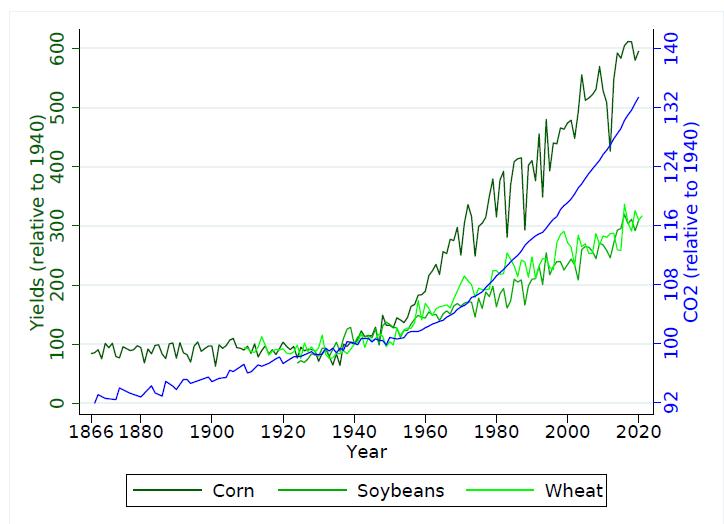
Figure 9.1: U.S. average CO2 levels and yields of corn, soy and wheat all normalized so 1940=100. Source: Taylor and Schlenker (2021)

Further evidence

A 2021 report from the U.S. National Bureau of Economic Research (Taylor and Schlenker 2021) used satellite-measured observations of outdoor CO2 levels across the United States, matched to county-level agriculturaloutput data and other economic variables. After controlling for the effects of weather, pollution and technology the authors concluded that CO2 emissions had boosted U.S. crop production since 1940 by 50 to 80 percent, attributing much larger gains than had previously been estimated using FACE experiments. They found that every ppmof increase in CO2 concentration boosts corn yields by 0.5 percent, soybeans by 0.6 percent, and wheat by 0.8 percent.

Beyond growth benefits, extra CO2 boosts plant resilience to dryness. See discussion in Section 2.1.3.

9.3 Crop modeling meta-analyses

Notwithstanding the abundant evidence for the direct benefits of CO2 and of CO2-induced warming on crop growth, in 2023 the U.S. Environmental Protection Agency (EPA 2023) boosted its estimate of the Social Cost of Carbon (SCC) about five-fold based largely on a very pessimistic 2017 estimate of global agricultural damages from climate warming (Moore et al., 2017). One of the two damage models used by the EPA attributednearly half ofthe 2030SCCto projected global agricultural damages based on the Moore et al. (2017) analysis. This study was a meta-analysis of crop model studies simulating yield changes for agricultural crops under various climate warming scenarios. Moore et al. projected declining global crop yields for all crop types in all regions due to warming.

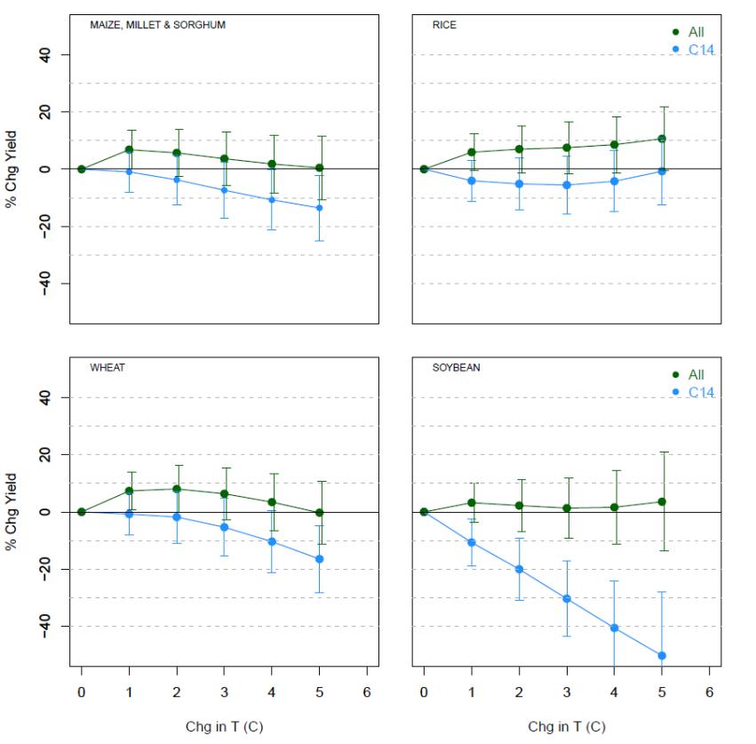
Figure 9.2 Crop yields under CO2-induced climate warming. Blue: as published in Moore et al. (2017). Green: after including omitted data. Source: McKitrick (2025).

McKitrick (2025)re-examined the Moore et al. database and found that, while it claimed to cover 1,722 studies, only half the entries (N=862) had complete records, so that the sample available for regression analysis was much smaller than both studies indicated. McKitrick noted that the records most commonly missing were the changes in ambient CO2 and found that in many cases these could be recovered from the underlying studies or the original climate scenario tables, thereby increasing the usable sample size by 40 percent. The crop yield projections incorporating the newly available data changed considerably. As shown in Figure 9.2, whereas the partial data set implied warming would decrease yield (blue lines), the complete data set implied constant or increase global yields, even out to 5°C warming (green lines).

9.4 CO2 fertilization and nutrient loss

Evidence has shown that CO2-induced biomass gains are sometimes accompanied by reductions in the concentrations of protein and other key nutrients such as iron and zinc (Ebi et al. 2021). Some experiments have shown that the rising temperatures expected to accompany higher CO2 levels will offset this loss (Köhler et al. 2019)althoughtheevidenceforthisismixed,asistheevidencethatnutrientdilutionobserved to date is entirely attributable to higher CO2 (Ziska 2022). If nutrient dilution does occur under rising CO2 levels, there are several adaptive strategies that could be pursued.

First, selective breeding to raise micronutrient content is already established (Saltzman et al. 2017) and has proven to be a cost-effective agronomic strategy (Ebi et al. 2021). Strategies can include both conventional breeding and genetically-modified organisms. An example of the latter is Golden Rice, which

contains elevated levels of beta-carotene to boost biosynthesis of vitamin A in the human body. Optimal strategies will be location-specific because they vary by crop, climate and soil type (Ebi et al. 2021). Second, fortification of food products with micronutrients is already routine. Folic acid (a B vitamin) is added to flour and many other foods; iodine is added to table salt, most commercial breakfast cereals are fortified with iron and numerous vitamins, etc. Third, dietary supplements in the form of multivitamin tablets are inexpensive, widely-available and routinely consumed.

One concern aboutreliance on adaptive strategies is whether they are feasible in low-income countries. Micronutrientdeficiency is alreadya problem in thedeveloping world and dietary supplements have proven to be an effective low-cost response (Ebi et al. 2021). It should also be noted the IPCC emission scenarios that generate high levels of warming also involve strong income growth. The SSP scenarios3 assume that, compared to 2005 levels, global per capita income will double by 2100 in the lowest growth case (SSP3), and in the highest emission case (SSP5) global per-capita income will grow nearly 16-fold. In that scenario eventhepoorestregions(AfricaandtheMiddleEast) endupwithapercapitaincomeofaboutUS$126,000, 70 percenthigher than current U.S. per capita income (aboutUS$75,000). Consequently the same scenarios in which CO2 levels increase the most are also those in which global poverty is largely eliminated, in which case all countries would be able to afford dietary supplements as necessary to address micronutrient deficiencies, if they arise and cannot be addressed using on-farm agricultural strategies.

In summary, there is abundant evidence going back decades that rising CO2 levels benefit plants, including agricultural crops, and that CO2-induced warming will be a net benefit to U.S. agriculture. To the extent nutrient dilution occurs there are mitigating strategies available that will need to be researched and adapted to local conditions.

References

Ainsworth, Elizabeth and Stephen P. Long (2020) 30 years of free-air carbon dioxide enrichment (FACE): What have we learned about future crop productivity and its potential for adaptation? Global Change Biology https://doi.org/10.1111/gcb.15375

Allen Jr, L. K. (2011). Elevated CO2 increases water use efficiency by sustaining photosynthesis of waterlimited maize and sorghum. Journal of Plant physiology, 168(16), 1909-1918.

Bareille, F. and R. Chakir (2023) The impact of climate change on agriculture: A repeat-Ricardian analysis. Journal of Environmental Economics and Management 119

Blandino, M. B. (2020). Elevated CO2 impact on common wheat (Triticum aestivum L.) yield, wholemeal quality, and sanitary risk. Journal of agricultural and food chemistry, 68(39), 10574-10585.

Burke, Marshall and Kyle Emerick (2016) Adaptation to Climate Change: Evidence from US Agriculture. American Economic Journal: Economic Policy 8(3) August 2016 106 140 https://www.aeaweb.org/articles?id=10.1257/pol.20130025

Cheng, L., Zhang, L.,Wang,YP. et al. Recent increases interrestrial carbon uptake at little costto thewater cycle. Nature Communications 8, 110 (2017). https://doi.org/10.1038/s41467-017-00114-5

CO2Science.org (undated) Plant growth archive http://www.co2science.org/data/plant_growth/dry/dry_subject_b.php

Deryng, D., Elliott, J., Folberth, C. et al. (2021) Regional disparities in the beneficial effects of rising CO2 concentrations on crop water productivity. Nature Climate Change 6, 786–790 (2016). https://doi.org/10.1038/nclimate2995

Deschênes, Olivier and Michael Greenstone (2012) The Economic Impacts of Climate Change: Evidence from Agricultural Output and Random Fluctuations in Weather: Reply to Comment American Economic Review 102, no. 7: 3761-3773. http://hdl.handle.net/1721.1/82641

3 See compilation at Our World in Data

Ebi, Kristie L, C Leigh Anderson, Jeremy J Hess, et al. (2021) Nutritional quality of crops in a high CO2 world: an agenda for research and technology development Environmental Research Letters 16(6) 064045 https://iopscience.iop.org/article/10.1088/1748-9326/abfcfa

Köhler, Iris H., Steven C. Huber, Carl J. Bernacchi, Ivan R. Baxter (2019) Increased temperatures may safeguard the nutritional quality of crops under future elevated CO2 concentrations The Plant Journal 97(5) 872 – 886 https://onlinelibrary.wiley.com/doi/epdf/10.1111/tpj.14166

Li, D. L. (2013). Effects of elevated CO2 on the growth, seed yield, and water use efficiency of soybean (Glycine max (L.) Merr.) under drought stress. Agricultural Water Management, 129, 105-112.

McKitrick, RossR. (2025) Extended CropYield Meta-analysis Data do notSupportUpwardSCCRevision. Scientific Reports 15 article 5575 https://www.nature.com/articles/s41598-025-90254-2

Mendelsohn, R., Nordhaus, W. D., & Shaw, D. (1994). The impact of global warming on agriculture: a Ricardian analysis. The American Economic Review, Sept 1994 753-771.

MooreFC,BaldosU,HertelT,DiazD(2017)Newscienceofclimatechangeimpactsonagricultureimplies higher social cost of carbon. Nature Communications 8:1607. https://doi. org/10. 1038/s41467-01701792-x

Ortiz-Bobea, Ariel (2019) The role of nonfarm influences in ricardian estimates of climate change impacts on US agriculture. American Journal of Agricultural Economics. 102 (3), 934–959.

Saltzman, Amy, Ekin Birol, Adewale Oparinde et al. (2017) Availability, production, and consumption of crops biofortified by plant breeding: current evidence and future potential. Annals of the New York Academy of Sciences Volume 1390, Issue1 https://doi.org/10.1111/nyas.13314

Schlenker, Wolframand Michael Roberts (2009) Nonlinear temperature effects indicate severe damages to U.S. crop yields under climate change. Proceedings of the National Academy of Sciences 106 (37) 15594-15598 https://doi.org/10.1073/pnas.0906865106

Taylor, Charles and Wolfram Schlenker (2023) Environmental drivers of agricultural productivity growth: CO2 fertilization of US field crops. National Bureau of Economic Research Working paper 29320, https://www.nber.org/papers/w29320

US Environmental Protection Agency (2023) Supplementary Material for the Regulatory Impact Analysis for the Final Rulemaking, “Standards of Performance for New, Reconstructed, and Modified Sources and Emissions Guidelines for Existing Sources: Oil and Natural Gas Sector Climate Review”, EPA Report on the Social Cost of Greenhouse Gases: Estimates Incorporating Recent Scientific Advances, Nov. 2023, https://www.epa.gov/system/files/documents/2023-12/epa_scghg_2023_report_final.pdf

Zhang et al. (2024) Less than 4% of dryland areas are projected to desertify despite increased aridity under climate change. Nature Communications Earth and Environment 5 June 2024 https://www.nature.com/articles/s43247-024-01463-y

Ziska, Lewis H (2022) Rising Carbon Dioxide and Global Nutrition: Evidence and Action Needed. Plants 1(7), 1000; https://doi.org/10.3390/plants11071000

10 MANAGING RISKS OF EXTREME WEATHER

Chapter summary

Trends in losses from extreme weather and climate events are dominated by population increases and economic growth. Technological advances such as improved weather forecasting and early warning systems have substantially reduced losses from extreme weather events. Better building codes, flood defenses, and disaster response mechanisms have lowered economic losses relative to GDP. The U.S. economy's expansion has diluted the relative impact of disaster costs, as seen in the comparison of historical and modern GDP percentages. Heat-related mortality risk has dropped substantially due to adaptive measures including the adoption of air conditioning, which relies on the availability of affordable energy. U.S. mortality risks even under extreme warming scenarios are not projected to increase if people are able to undertake adaptive responses.

10.1 Socioeconomic context

Risks from human-caused climate change are affected by natural weather and climate variability and are dominated by the exposure of wealth in coastal and other disaster-prone regions and vulnerabilities of poorer populations. The evolution of climate risk in the U.S. has been dominated by societal factors, rather than by changes to the actual weather and climate hazards. Deaths from weather disasters have decreased substantially since 1900, even as U.S. population grew from 76 million in 1900 to over 331 million in 2020 (Goklany 2011). For example, the Galveston hurricane killed over 8,000 people in 1900 (0.01 percent of the U.S. population), whereas the worst recent disaster, Hurricane Katrina in 2005, killed 1800 people (or 0.0006percentoftheU.S.population)(NOAANationalHurricaneCenter2025;U.S.CensusBureau2025).

Technologicaladvances have substantially reduced lossesfrom extreme weather events. Early warning systems, satellite monitoring, and improved weather forecasting have reduced deaths, although exact numbers are hard to quantify (Deryugina and Hsiang 2023). U S weather forecasting has been estimated to reduce losses from weather events with an annualized benefit of $31.5B, protecting lives, property, and supporting agriculture and transportation (NRC 2010). Improved hurricane forecasts have reduced preand post-landfall spending, with annual per hurricane cost reductions estimated at $5B (Molina and Rudik 2024).

Infrastructure improvements have contributed to substantial reductions in losses from extreme weather events. Building codes, suchas those implemented in Florida after Hurricane Andrew(1992), havereduced losses by ensuring structures can withstand high winds and floods. Homes built after 2002 showed minimal damage during Hurricane Michael (2018), unlike older homes (FEMA 2020). Sea walls, like the Galveston Seawall, protect against wave action and storm surge. The New Orleans Hurricane and Storm Damage Risk Reduction System successfully mitigated storm surge during Hurricane Isaac (2012) (Battelle Memorial Institute 2013). Inland dams in the U.S. help control flooding by storing excess water during heavy rains. It is estimated that the Tennessee Valley Authority (TVA) dams prevent about $309M in annual flood damage in the TVA region and along the Ohio and Mississippi Rivers (TVA, 2025). During Hurricane Helene (2024), TVA’s strategies prevented approximately $406M in potential damages (APPA 2024).

10.2 Data challenges

Since 1980, NOAA has provided a count of annual U.S. weather-related disasters that it estimates to have exceeded $1 Billion (inflation adjusted), showing a substantial increase starting in 2008. NOAA and other government officials have cited the upward trend in the Billion Dollar Disaster series as evidence that climate change is making extreme weather worse (Pielke Jr., 2024). But over time, population and wealth have increased dramatically in the U S , so when an extreme weather or climate event occurs, there is more damage even if there is no underlying trend in the frequency or intensity of extreme weather. Pielke Jr. (2024) demonstrates that losses per weather disaster as a proportion of GDP have decreased by about 80 percent since 1980, as shown in Figure 10.1 Pielke Jr. (2024) also argued that in addition to relying on opaque data sources and unreported adjustments, NOAA failed to normalize its Billion Dollar Disaster data series properly for changes in population exposure and wealth. In May 2025 NOAA announced it has withdrawn the Billion Dollar Disaster product from publication (Pielke Jr., 2025).

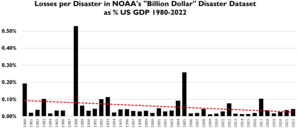
In summary, trends in losses from extreme weather and climate events are dominated by population increases and economic growth. Technological advances such as improved weather forecasting and early warning systems have substantially reduced losses from extreme weather events. Better building codes, flood defenses, and disaster response mechanisms have lowered economic losses relative to GDP. Finally, the U.S. economy's expansion has diluted the relative impact of disaster costs, as seen in the comparison of historical and modern GDP percentages.

10.3 Mortality from temperature extremes

10.3.1

Heat and cold risks

Changes in temperature extremes are among the most certain impacts expected in a warming world. It stands to reason that extreme heat events would likely become more frequent while extreme cold events would become less frequent. This pattern is evident in the historical period, though not in the continental U.S. (Chapter 6), and is expected to continue with further warming.

Figure 10.1: Losses per disaster as a % of Gross Domestic Product in NOAA’s billion-dollar disaster dataset (the version downloaded in July 2023), 1980 to 2022. Source: (Pielke, Jr. 2024)

Mortality during heat extremes is typically caused by heat stroke and heat exhaustion, while mortality during cold extremes typically stems from hypothermia and heart strain. Global mortality is substantially greater for cold conditions than for hot conditions (Zhao et al 2021, Ritchie 2024). Unlike with heat-related mortality, cold-weather risks set in even at moderately cold conditions (Gasparini et al. 2015, Lee and Dessler 2023). The U S EPA (citing data from the Centers for Disease Control) reports that on average over 1999 to 2015 there were 2.2 deaths per million Americans for which cold was listed as the main underlying cause and an additional 2.4 deaths per million for which cold was listed as a contributing factor (EPA 2025). By contrast there were 1.3 deaths per million for which heat was the main cause and an additional 0.8 per million for which it was a contributor. By this metric cold accounts for approximately double the weather-related deaths as does heat.

Epidemiologicalmethodsthatconsidercorrelationalevidence,notjustdeathcertificatereports,indicate the cold/warm ratio might be much higher. A 13-country study of 74 million deaths from 1985 to 2012 estimated that, on average, 7.7 percent of deaths were attributable to sub-optimal temperatures, of which 7.4 percent were attributable to cold and only 0.4 percent were attributable to heat (Gasparini et al. 2015). In other words, cold weather killed 18.5 times as many people as did hot weather.

Figure 10.2 shows the distribution of results from Gasparini et al. (2015) by country. For the United States the fraction of deaths attributable to temperature was 5.9 percent, of which 5.5 percent was due to cold, thus cold weather killed 14 times as many people as hot weather.

Figure 10.2. Mortality attributable to extreme and moderate cold and heat by country. Source: reproduced from Gasparini et al. (2015).

There is strong evidence that people adapt to weather risks. Lee and Dessler (2023) reported that 86 percent of temperature-related deaths across 40 cities in the U.S. were due to cold-related mortality, and that due to adaptation the relative risk of death declined in hot and cold cities alike as seasonal temperatures increased. Allen and Sheridan (2018) found that short, early-season cold events were 2 to 5 times deadlier than hot events, but the mortality risk of both cold and hot extremes drops to nearly zero if the events occur late in the season.

Davis et al. (2003) examined heat-related mortality in 28 U.S. cities from the 1960s to the end of the 1990s and found that heat-related mortality declined by three-quarters over the sample period. Bobb et al. (2014) examined mortality data for 106 million people in over 100 cities U.S. cities and found a 60 percent decline in average heat-related mortality over the period 1987 2005, from 51 per thousand deaths to 19. They furthermore foundthatthe greatestdropwasamongseniors overtheage of 75. In astudy of 42 million

deaths in 211 U.S. cities from 1962 to 2006. Nordio et al. (2015) found a more than 90 percent decline in the risk of mortality from excess heat.

In the context of large declines in heat-related mortality, rising temperatures are associated with a net saving of lives since they reduce mortality from cold events. AR6 Working Group 2 Chapter 16.2.3.5 (O’Neill et al. 2022) acknowledges that heat-related mortality risk is declining over time:

Heat-attributable mortality fractions have declined over time in most countries owing to general improvements in health care systems, increasing prevalence of residential air conditioning, and behavioral changes. These factors, which determine the susceptibility of the population to heat, have predominated over the influence of temperature change.

Yetthe IPCCmisrepresents the overall situation in its AR6Synthesis report.Section A.2.5 of thatdocument states:“In allregions increases inextremeheat events have resulted in human mortality and morbidity (very high confidence).” But it is silent on the larger decline of deaths during extreme cold events.

The observed decline in U.S. heat-related mortality has been specifically attributed to adaptation. Wang et al. (2018) exploited the spatial variability of heatwave-related mortality across 209 U.S. cities from 1962 to 2006. While simple correlation appeared to imply an increase in mortality risk during heatwaves, accountingforadaptation to heatwave intensitycausedtheeffect tofall to near zero andbecome statistically insignificant. They used the results of their epidemiological model to project heat-related mortality out to 2050 under four RCP warming scenarios (including RCP8.5) with and without adaptive behavior. Assuming people continue to adapt to the heatwave risks in the regions in which they live. Wang et al. (2018) project not only no increase in heat-related mortality, but an overall mortality decrease for the U S. They conclude that

Ignoring adaptation would result in a substantial overestimate of future mortality related to heat waves… Accounting for adaptation, the overall heat-related mortality by 2050 would not change substantially over time compared to 2006.

10.3.2 Mortality risks and energy costs

A 2016 study of U S long term mortality risks associated with temperature variations (Barreca et al. 2016) showed that increases in mortality across the U S are associated with both cold weather and hot weather. But over time, the introduction of electricity and the adoption of central heating and air conditioning (AC) dramatically reduced both risks, especially those associated with hot weather. Prior to 1960 a day above 90°F (32°C) added 2.2 percent to the average mortality risk rate, but after 1960 the same weather added only 0.3 percent to mortality risk, an 85 percent reduction. Prior to 1960 temperatures below 39°F (4°C) added about 1 percent to mortality risk but after 1960 the same weather only added about half that amount. Adaptation through conventional household improvements dramatically reduced public vulnerability to weather extremes. The entire reduction in hot weather mortality was attributable to widespread adoption of indoor AC,which dependedon theavailability ofreliableandaffordable electricity.

The corollary of this finding is that the use of heating and cooling systems depends on energy being affordable. Doremus et al. (2022) showed that wealthy and poor households in the U.S. adjust their energy expenditures at similar rates in response to moderate temperature swings, but not in response to extreme temperature swings. When temperatures swing to very cold levels (< 5°C) energy spending in high-income

households rises by 1.2 percent but in low-income households by only 0.5 percent. On very hot days (>30°C) electricity spending in high-income households rises by 0.5 percent but does not change at all in low-income households. The latter result is observed even in subsamples where all households have AC. Cong et al. (2022) report similar findings for a sample of households in Arizona. The implication is that even with widespread adoption of home heating and cooling systems, inability to afford energy leaves lowincome households exposed to weather extremes.

References

Allen, M.J. and S.C. Sheridan (2018) Mortality risks during extreme temperature events (ETEs) using a distributed lag non-linear model. (2018) International Journal of Biometeorology 62, 57–67 (2018). https://doi.org/10.1007/s00484-015-1117-4

American Public Power Association. (APPA, 2024, March 7). TVA flood mitigation strategies prevented approximately $406 million in potential damages. Public Power Current. https://www.publicpower.org/periodical/article/tva-flood-mitigation-strategies-preventedapproximately-406-million-potential-damages

Barreca,Alan,KarenClay,OlivierDeschenes,MichaelGreenstone,andJosephSShapiro (2016),Adapting to climate change: The remarkable decline in the US temperature mortality relationship over the twentieth century, Journal of Political Economy, 2016, 124 (1), 105–159.

Battelle Memorial Institute. (2013, December). Final independent external peer review report: Hurricane Isaac (2012) assessment (Prepared for U.S. Army Corps of Engineers, New Orleans District). https://www.mvn.usace.army.mil/Portals/56/docs/PD/PeerReview/TCN13003HurrIsaacAssessIEPRFinal.pdf

Bobb JF, RD Peng, ML Bell and F Dominici (2014) Heat-related mortality and adaptation to heat in the United States. Environmental Health Perspectives 122:811–816; https://ehp.niehs.nih.gov/doi/full/10.1289/ehp.1307392

Cong, S., D. Nock, Y.L. Qiu, Y.L. et al. Unveiling hidden energy poverty using the energy equity gap. Nature Communications 13, 2456 (2022). https://doi.org/10.1038/s41467-022-30146-5

Davis, Robert E., Paul C. Knappenberger, Patrick J. Michaels and Wendy M. Novicoff (2003) “Changing Heat-Related Mortality in the United States” Environmental Health Perspectives 111(14) November 2003 pp. 1712 1718 https://ehp.niehs.nih.gov/doi/pdf/10.1289/ehp.6336

Deryugina, T., & Hsiang, S. M. (2023). Does the environment still matter? Daily temperature and income in the United States (NBER Working Paper No. 31361). National Bureau of Economic Research. https://www.nber.org/papers/w31361

Doremus, JM, I. Jacqz and S. Johnston (2022), “Sweating the energy bill: Extreme weather, poor households, and the energy spending gap.” Journal of Environmental Economics and Management, doi: https://doi.org/10.1016/j.jeem.2022.102609

Environmental Protection Agency (2025) Climate Change Indicators. https://www.epa.gov/climateindicators/view-indicators

Federal Emergency Management Agency (FEMA). (2020, February 13). The role of Florida’s building codes in Hurricane Michael recovery. https://www.fema.gov/case-study/role-floridas-building-codes2018-hurricane-michael

Gasparini, A., Y. Guo, M. Hashizume et al. (2015) Mortality risk attributable to high and low ambient temperature: a multicountry observational study The Lancet 386: 369-385 July 25, 2015 http://dx.doi.org/10.1016/S0140-6736(14)62114-0

Goklany, I. M. (2011). Deaths from extreme weather events, 1900–2010. Reason Foundation. https://a8d50b36.delivery.rocketcdn.me/wpcontent/uploads/2011/09/deaths_from_extreme_weather_1900_2010.pdf

Lee, Jangho and Andrew Dessler (2023) Future Temperature-Related Deaths in the U.S.: The Impact of Climate Change, Demographics, and Adaptation GeoHealth 7(8) August 2023 https://doi.org/10.1029/2023GH000799

Molina, R and I Rudik (2024) The value of improving hurricane forecasts. National Bureau of Economic Research Working Paper 32548 June 2024 https://www.nber.org/digest/202409/value-improvinghurricane-forecasts

National Hurricane Center. (n.d.). Costliest U.S. tropical cyclones tables updated. NOAA National Hurricane Center. Retrieved May 8, 2025, from https://www.nhc.noaa.gov/outreach/history/ National Research Council. (2010). Adapting to the impacts of climate change. The National Academies Press. https://nap.nationalacademies.org/read/12888/chapter/2

Nordio, Francesco, Antonella Zanobetti, Elena Colicino, Itai Kloog and Joel Schwartz (2015). “Changing patterns of the temperature–mortality association by time and location in the US, and implications for climate change” Environment International Volume 81, pp 80-86 https://doi.org/10.1016/j.envint.2015.04.009

O'Neill, B., et al. (2022). Key risks across sectors and regions. In AR6 Working Group II Climate Change 2022: Impacts, Adaptation and Vulnerability (pp. 2411–2538). Intergovernmental Panel on Climate Change. www.ipcc.ch

Pielke Jr., R. (2024). Scientific integrity and U.S. 'billion dollar disasters'. npj Natural Hazards, 1, Article 12. https://www.nature.com/articles/s44304-024-00011-0

Pielke Jr., R. (2025, May 8). RIP NOAA's billion dollar disasters. The Honest Broker [Substack]. https://rogerpielkejr.substack.com/p/rip-noaas-billion-dollar-disasters Ritchie, H. (2024). How many people die from extreme temperatures, and how this could change in the future: Part one. Our World in Data. https://ourworldindata.org/part-one-how-many-people-die-fromextreme-temperatures-and-how-could-this-change-in-the-future

Tennessee Valley Authority (TVA). (n.d.). Flood management. Retrieved May 8, 2025, from https://www.tva.com/environment/managing-the-river/flood-management

U.S. Census Bureau. (n.d.). Decennial census by decade. Retrieved May 8, 2025, from https://www.census.gov/programs-surveys/decennial-census/decade.html

Wang, Yan, Francesco Nordio , John Nairn , Antonella Zanobetti and Joel D. Schwartz(2018) “Accounting for adaptation and intensity in projecting heat wave-related mortality” Environmental Research 161 pp. 464 471. https://doi.org/10.1016/j.envres.2017.11.049

Zhao, Q., et al. (2021). Global, regional, and national burden of mortality associated with non-optimal ambient temperatures from 2000 to 2019: A three-stage modelling study. The Lancet Planetary Health, 5(7). https://doi.org/10.1016/s2542-5196(21)00081-4

11 CLIMATE CHANGE

, THE ECONOMY, AND THE SOCIAL COST OF CARBON

Chapter summary

Economists have long considered climate a relatively unimportant factor in economic growth, a view echoed by the IPCC itself in AR5. Mainstream climate economics has recognized that CO2-induced warming might have some negative economic effects, but they are too small to justify aggressive abatement policy and that trying to “stop” or cap global warming even at levels well above the Paris target would be worse than doing nothing. An influential study in 2012 suggested that global warming would harm growth in poor countries, but the finding has subsequently been found not to be robust. Studies that take full account of modeling uncertainties either find no evidence of a negative effect on global growth from CO2 emissions or find poor countries as likely to benefit as rich countries.

Social Cost of Carbon (SCC) estimates are highly uncertain due to unknowns in future economic growth, socioeconomic pathways, discount rates, climate damages, and system responses. The SCC is not intrinsically informative as to the economic or societal impacts of climate change. It provides an index connecting large networks of assumptions about the climate and the economy to a dollar value. Some assumptions yield a high SCC and others yield a low or negative SCC (i.e. a social benefit of emissions). The evidence for or against the underlying assumptions needs to be established independently; the resulting SCC adds no additional information about the validity of those assumptions. Consideration of potential tipping points does not justify major revisions to SCC estimates.

11.1 Climate change and economic growth

11.1.1 Overview

It has long been noted that economies tend to do poorly in very cold and very hot regions, with the optimum somewhere in between (Nordhaus, 2006). This implies that warming will tend to be harmful in hot regions but beneficial in cool ones. Temperature-sensitive economic activity migrates, whenever possible, to where it is best suited, and society adapts to the local climate. Based in part on these observations, in 1992 Thomas Schelling, then President of the American Economic Association, argued that any effects of climate change on U.S. economic activity would be small relative to the many other changes that would happen (Schelling 1992)

… Manufacturing rarely depends on climate, and where temperature and humidity used to make a difference, air conditioning has intervened. When Toyota chooses among Ohio, Alabama, and Southern California for locating an automobile assembly, geographical considerations are important, but not because of climate... Finance is little affected by climate; similarly for health care, or education, or broadcasting. Transportation can be affected, but improvements in allweather landingand take-off in the last30yearsaregreaterthan anydifferencesthat climatemakes. If the average effect is a warming, iced waterways and snow removal may decline in importance.

Construction is affected, mainly by cold, and if the average effect is in the direction of warming, construction may benefit slightly.

It is really agriculture that is affected. But even if agricultural productivity declined by a third over the next half century, the per capita GNP we might have achieved by 2050 we would achieve only in 2051. …

I conclude that in the United States, and probably Japan, Western Europe, and other developed countries, the impact on economic output will be negligible and unlikely to be noticed.

Thirty years later virtually the identical point was made by the IPCC itself in the Fifth Assessment Report (Arent et al. 2014, emphasis added)

For most economic sectors, the impact of climate change will be small relative to the impacts of other drivers. Changes in population, age, income, technology, relative prices, lifestyle, regulation, governance,and many otheraspects of socioeconomic development will havean impact on the supply and demand of economic goods and services that is large relative to the impact of climate change.

Evidence since AR5 does not change this assessment. Mohaddes et al. (2023) found that warm weather shocks have small negative effects on U.S. state-level output but not income, while cold weather shocks negatively affect both and the impacts are about four times larger, implying a shift to warmer conditions would, if anything, yield a net economic benefit for the U.S.

These statements are validated by experience. Since 1900, the average global surface temperature anomaly warmed 1.3°C, about as muchas the IPCCpredicts will occur in the nextcentury under a moderate emissions scenario. But even as the globe warmed and the population quintupled, humanity prospered as never before. For example, global average lifespan went from thirty-two years to seventy-two years, economic activity per capita grew by a factor of seven, and the death rate from extreme weather events plummeted by a factor of fifty. Climate change damage projections typically refer to reductions in how much life will improve for humanity, they don’t state that it will get worse in an absolute sense (O’Neill 2023).

While extreme weather events are costly, in all modern economies they are becoming steadily less and less important (Formetta and Feyen, 2019). Since 1990 weather-related disaster losses have declined as a proportion of global GDP (Pielke Jr , 2018, 2020) as have mortality risks (Formetta and Feyen, 2019). While economic weather-related insurance payouts are rising, this is fully explained by the growth in the size of the economy and the value of the insured asset stock. Past increases in episodes extreme weather have not had a significant effect (positive or negative) on the market value of insurance firms (Hu and McKitrick, 2015). Nor have past extreme weather events had a significant effect on U.S. banks’ performance (Blickle et al., 2021); warming has even been shown to be beneficial for the finance and insurance sector (Mohaddes et al. 2023) Figure 11.1 below is illustrative For these reasons, economists have long been reluctant to endorse attempts to “stop” climate change or even aggressively reduce GHG emissions because the costs would not be worth it. As one critic of the economics of climate policy put it (Storm 2017):

Mainstreamclimateeconomics takes global warming seriously, but perplexingly concludes that the optimal economic policy is to almost do nothing about it… The contrast is striking. While climate science is sending outloud-and-clear messages thatfossil-fuel disinvestmentmuststart now,letting

go of coal and oil and diverting resources into renewable energy technology systems, to keep warming below the 2°C limit (IPCC 2014), mainstream climate economics claims that overly ambitious climate targets will unnecessarily hurt the economy and immediate de-carbonization is too expensive. Most climate economists thus recommend humanity to just wait-and-see.

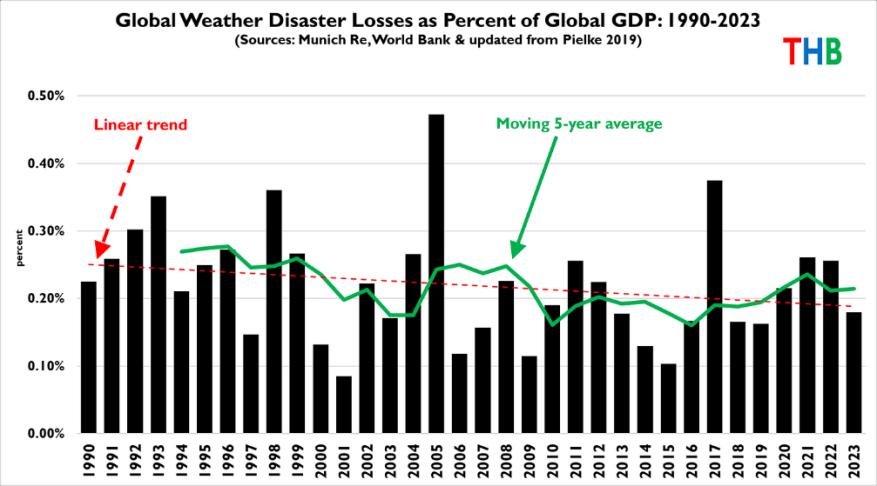
Figure 11.1 Global weather losses as a fraction of GDP. Source: Pielke Jr. (2023)

The mainstream economics position on the climate policy question is best represented by the findings over the pastthree decades from Integrated Assessment Models (IAMs) of climate change policy, for which Yale economist William Nordhaus was awarded the 2018 Nobel Memorial Prize in economics. IAMs combine economic, climate, and social data into a unified framework for simulating climate damages and evaluating the optimal policy response (Resources for the Future, 2025). Nordhaus’ work has generally supported modest global climate policy, with aggressive measures largely deferred to later in the century. Nordhaus developed theso-calledDynamic IntegratedModel of the Climateand Economy model, or DICE, in the early 1990s (Nordhaus, 1993) to study the interaction between climate change, climate policy, and global economic growth over long times. DICE assumes global emission control can be coordinated at no cost and asks what the optimal policy target should be. The climate component of the DICE model is based on simplified climatological modeling. The version of DICE at the time of Nordhaus’ Nobel Prize award was described in Nordhaus (2018); it had a climate sensitivity parameter of 3.1°C for CO2 doubling, consistent with the best estimate in IPCC reports (3.0°C).

The baseline (no policy) scenario incurs only $0.4T in global abatement costs and leads to $134.2T (trillion dollars) in global climate damages for a total cost of $134.6T. The climate model component of DICE projects 4.1°C warming by 2100 relative to preindustrial temperatures. Note that this is a higher estimate of warming than many IPCC climate models.

The Optimal Policy scenario barely deviates from the business-as-usual path. It aims for +3.5°C warming, in other words we modestly scale back fossil fuel use and otherwise just live with almost all the warming. This suggests that most CO2 emissions are less harmful than the policies that would be necessary to abate them. Trying to prevent warming causes costs quickly to outstrip the benefits. Pursuing a goal of capping warming at 2.5°C creates total costs of $177.8T, which is $43.2T worse than doing nothing at all. Nordhaus didn’t evaluate trying to reach a Paris-type target of 1.5°C warming but it would be even more costly

A subsequent edition of DICE includes higher assumed damages from warming which, not surprisingly leads to more aggressive policy recommendations, as explained in the section below on the Social Cost of Carbon.

11.1.2 Empirical analysis of climate change and economic growth

Many other studies have used econometric methods applied to historical data, instead of IAMs, to study the potential impact of climate change on economic growth. Dell et al. (2012, herein DJO12) was an influential study that used a multi-country panel of national-level data spanning 1950 to 2005, in which they matched climate and economic data by averaging temperature from the local grid cell level up to the national level using population weights. They found that warming yields an insignificant positive effect on income growth in rich countries but a significant negative effect in poor countries. Moore and Diaz (2015) modified the DICE model to take that finding into account and concluded that it implied a dramatically higher Social Cost of Carbon due to the compounding effects of income loss over time.

A large subsequent literature has debated the robustness of the DJO12 findings. Burke et al. (2015) analyzed a global panel with temperatures averaged up to the national level and found a negative effect on growth fromwarming in richandpoorcountriesalikewhen the national average temperatureis above 13°C. Zhao et al. (2018) used the G-Econ data set of Nordhaus (2006), which breaks economic activity down to the grid cell level, replicated DJO12-type results on the same subset of countries as used in DJO12 but then showed that on the full global sample warming increases growth in rich countries and poor countries alike, though the positive effect in the latter group is confined to where local temperatures are below about 16°C. Greβer et al. (2021) developeda regional economic data set for 1,542 sub-nationalregionsaround theworld between 2005 and 2015 and found temperature had no effect on growth. Yang et al. (2023) updated the DJO12 data setandapplied anestimator robustto mixed sample frequencies, finding that while temperature shocks exerted a temporary effect on income levels, they did not have a significant lasting effect on growth rates.

Newell et al. (2021) noted that there is no underlying theory to guide econometric model specification in this literature Taking into account the arbitrary choices of which explanatory variables to include, they identified over 800possible model specifications. Using the Burke et al. (2015)data theyusedanestimation method thataccounts for model uncertainty and found that the model form preferred by Burke et al. (2015), which implied negative effects of warming on growth even in rich countries, is explicitly excluded by the optimal model selection algorithm. Overall, they could not detect a temperature effect on GDP or GDP growth, and they estimated the 95 percent confidence interval for the impact on global growth as of 2100 even under the exaggerated RCP8.5 warming scenario spans −86 percent to +388 percent. In other words the net effect is likely positive but too uncertain to distinguish from zero.

Barker (2023) criticized the DJO12 assumption that countries can be grouped into fixed “poor” and “rich” categories based on their incomes many decades ago. He noted that many countries were once poor but became rich over time, and if this is considered the original temperature effects reported by Dell et al. became small and insignificant.

Berg et al. (2023) argued that countries shouldn’t be grouped into large Rich/Poor categories because they are too heterogeneous. They instead estimated country-specific temperature response coefficients then grouped countries with similar response coefficients into small panels. They separately estimated responses to global and idiosyncratic local temperature shocks to better identify the climate signal in weather data. Overall, they found countries experiencing negative effects of warming on growth outnumbered those experiencing positive effects, but only temporarily: eventually the effects reverse such that about twice as many countries experience a net positive growth effect. They also found global (as opposed to local) temperaturechangesaremuchmore likelytobenefitgrowthinpoorcountriesthanrichones. Inasimulation to 2100, even using the extreme RCP8.5 scenario, they computed the average global GDP loss would be

only 1.9 percent compared to a scenario with no warming. That is, instead of the economy growing 400 percent it would grow 392%. The implication of Nordhaus’ earlier analysis is that trying to prevent the warming would lead to far less than 392 percent growth.

To summarize, economists consider climate a relatively unimportant factor in economic growth, a view echoed by the IPCC itself in the Fifth Assessment Report. Mainstream climate economics has recognized that CO2-induced warming might have some negative economic effects but they are too small to justify aggressive abatement policy and trying to “stop” or cap global warming even at levels well above the Paris target would be worse than doing nothing. An influential study in 2012 suggested that global warming would harm growth in poor countries but the finding has subsequently been found not to be robust (Tol 2024). Studies that take full account of modeling uncertainties either find no evidence of a negative effect on global growth from CO2 emissions or find poor countries as likely to benefit from it as rich countries.

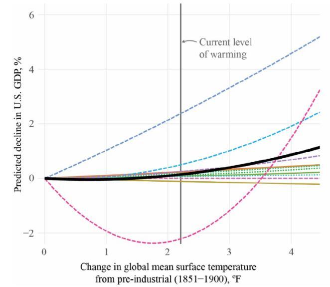
Figure 11.2: Decline in U.S. GDP per degree of warming. Source: CEA-OMB (2023)

The expectation that significant global warming would have a small impact on the U.S. economy was acknowledged quietly by the Biden Administration, even as the President was proclaiming a climate emergency. Figure 11.2, from a 2023 CEA-OMB report, shows the expected decrement in U.S. GDP as a function of temperature rise. The colored lines show the results of a dozen peer-reviewed published studies while the solid black line is their average. The figure could be summarized as “a few percent impact for a few degrees of warming”. Given that the economy’s annual growth rate is expected to be 1-2 percent, the impact of a warming globe on the U.S. GDP is indeed negligible.

11.2 Models of the Social Cost of Carbon

The Social Cost of Carbon (SCC) is a tool for quantifying the economic impact of carbon dioxide emissions, helping policymakers weigh the costs and benefits of climate policies. It estimates the damage caused by emitting one additional ton of CO₂, expressed in dollars. More formally, the SCC is the discounted present value of the current and future marginal loss of economic welfare due to an additional ton of CO2 entering the atmosphere.

11.2.1 Estimating the SCC

Although the literature refers to “estimates” of the SCC, it is not estimated in the way other economic statistics are estimated. For instance, data on market transactions including prices and quantities can be used to estimate the current inflation rate or the growth rate of per capita real Gross Domestic Product, and there are well-understood uncertainties associated with these quantities. But there are no market data available to measure many, if not most, of the marginal damages or benefits believed to be associated with CO2 emissions, so these need to be imputed using economic models.

For example, an influentialcomponent of some SCCcalculations is the perceived social costassociated with a changed risk of future mortality due to extreme weather. There is no market in which people can directly attach a price to that risk. At best economists can try to infer such values by looking at transactions in related markets such as real estate or insurance, but isolating the component of price changes attributable to atmospheric CO2 levels is very difficult.

Economists use IAMs to compute the SCC. Two of the best-known are the Climate Framework for Uncertainty, Negotiation and Distribution (“FUND”, Tol 1997) and Nordhaus’ DICE. EPA (2023) introduced new ones for its recent work. IAMs embed a “damage function” or set of functions relating ambient temperature to local economic conditions. The assumptions embedded in the damage function will largely determine the resulting SCC. IAMs also assume a long-term discount rate or, as in DICE, compute the optimal internal discount rate as part of the solution.

One approach to developing a damage function is to begin with estimates of the costs (or benefits) of warming in specific sectors in countries around the world and aggregate up to a global amount. This was the approach used in FUND. An alternative approach is to develop a simple equation that penalizes global income according to a simple quadratic function of the average global temperature. This approach was used in DICE. In the case of the FUND model many hundreds of parameters had to be selected, whereas in DICE only three were needed and were originally chosen to assign a predetermined penalty (1.2%) to global output as of 3°C warming, with a quadratic term implying that damages grow with the square of the global average temperature anomaly. Barrage and Nordhaus (2024) recently changed the parameters to increase the penalty at 3°C to 1.6%, and added a discrete additional 1.0 percent GDP penalty at 3°C warming to account for “tipping points” (discrete large-scale environmental changes triggered by crossing a warming threshold) and a “judgmental adjustment” of 0.5 percent for excluded impacts at 3°C warming. Not surprisingly the newer version of DICE generates much higher SCC estimates than before.

The concepts of estimation and uncertainty do not readily apply to SCC calculations. No amount of data collection can change the fact that many components of the SCC are unknown and rely on judgment and opinion based on knowledgeof the underlying literature on thephysicaleffects ofclimatechange. SCC calculations are thus best thought of as “if-then” statements: if the following assumptions hold, then the SCC is $X per tonne. The list of ‘if’ statements includes the premise that the world’s climate and economy workaccordingtotherepresentationintheIAM.Onewaythis mightfailtoholdis inthetimingofwarming. Every IAM assumes a value of the Equilibrium Climate Sensitivity (ECS), which controls the amount of warming that results from CO2 emissions and can be freely varied for the purpose of generating a distribution of SCCvaluesassociatedwith uncertainties over ECS.But as Roeand Baumann (2013) pointed out, time-to-equilibrium increases with the square of ECS, so an upward adjustment of the ECS parameter without an appropriate slowing down of the adjustment process can yield distorted present value damage estimates. In particular, the upper tail of warming associated with some commonly-used ECS distributions is physically impossible for even a thousand years into the future (Roe and Baumann 2013) yet in an IAM would be realized within a couple of centuries. Failure to align ECS with time-to-equilibrium will lead to an overestimate of the SCC value.

11.2.2 Variations in the SCC

Every level of the IAM calculation includes assumptions, some more influential than others. Key assumptions include the following.

• The discount rate: Climate damages accrue over a long time horizon and costs a century or two in the future need to be discounted to the present. The higher the discount rate the smaller the present value of future damages and vice versa. The discount rate represents the opportunity cost of spending money today rather than investing it and then having more to spend tomorrow. Some economists have argued for the use of very low discount rates in SCC calculations, resulting in policy recommendations that favor relatively large immediate investments in CO2 emission reductions. The downside is that other investments could potentially earn a larger rate of return for society.

• Equilibrium Climate Sensitivity: IAMs have customarily employed a value of 3.0°C or 3.1°C following the IPCC’s guidance The most recent data-driven ECS values tend to be lower than this (see Chapter 4). Dayaratna et al. (2017, 2020, 2023) have shown that use of lower empiricallyderived ECS values dramatically lower the resulting SCC estimate, even when low discount rates are used.

• Damage function coefficients: IAMs assume CO2 and warming cause net harms that increase exponentially with temperature. More recently, IAMs have also incorporated effects from assumed potential climate tipping points. The FUND model took limited but explicit account of CO2 fertilization effects in agriculture. Since the coefficients were selected prior the publication of the current evidence of global greening and the magnitude of benefits to crops from elevated CO2 (see Chapters 2 and 9) the growth effects are likely understated. The DICE model (and others) did not explicitly include any CO2 fertilization benefit, except to the extent it was taken into account in the literature consulted when picking the damage function coefficients. The damage function in FUND contains a region in which low warming yields net benefits in many regions, a finding which is supported by econometric models of warming and growth (Berg et al. 2023) and econometric simulations of agriculturalchanges(McKitrick 2025).TheDICE damagefunction, by construction, rules out net benefits at any warming level.

• Emission scenarios: IAMs generate SCC estimates that increase as the pre-existing concentration of CO2 increases. Consequently the value of damages later in the century will be higher, depending on the assumed baseline emissions over the coming decades.

Some IAMs (such as DICE) include the cost to the economy of reducing CO2 emissions in order to identify the SCC along an optimal growth path If CO2 emission reductions are assumed to be inexpensive, then the model will conclude that the optimal policy should aim for deeper emission cuts and vice versa.

It is informative to ascertain whether SCC results are invariant to changes in some assumptions. But when different assumptions result in higher or lower SCC values, the change in the SCC value does not provide prima facie evidence about the validity of the assumptions. For example, in 2023 the U.S. Environmental Protection Agency raised its preferred SCC value about 5-fold over the estimates it had issued ten years earlier. This is not because new data had been collected or better mathematical methods had been invented, but because new assumptions had been used, and the validity of those assumptions was a separate question. Tabulations on EPA (2023) p. 81 show that if assumptions similar to earlier analyses had been applied, the results would not have materially differed from before. One new assumption was that global agricultural damages were far higher than previously believed, based on an analysis in Moore et al. (2017). But as discussed in Chapter 9, McKitrick (2025) showed that Moore et al. (2017) had used a database in which half the CO2 change observations were missing. When as many of those observations as possible were recovered from underlying sources and the analysis was rerun, the projected crop yield losses disappeared and turned into gains at all warming levels. Hence the portion of the EPA’s SCC revision attributable to agricultural yield losses was unwarranted.

11.2.3 Evidence for low SCC

Chapter 2 reviewed evidence on climate change and greening, and Chapter 9 looked at climate change and U S agriculture. Evidence shows that CO2 fertilization has a stronger beneficial effect on agriculture than was known at the time that IAMs like DICE and FUND were parameterized. Haverd et al. (2020) found the observed CO2 fertilization rate has been almost double what had been predicted by crop models. Dayaratna et al. (2023) used the updated empirical ECS distribution estimate of Lewis (2022), which assimilates modern instrumental and paleoclimatic temperature records, and allowed for a 30 percent gain in the CO2 fertilization benefit in the FUND model, and found that, even at a low discount rate of 2.5 percent, the median SCC as of 2050 is only $18.67, with a 24 percent probability of the true value being negative. At a five percent discount rate the median SCC value is negative until the mid-2040s and at 2050 was only $0.37 with a 49 percent probability of being negative. Thus, under reasonable assumptions a mainstream IAM using updated scientific inputs yields evidence consistent with the SCC not being significantly greater than zero.

It should also be noted that the SCC is focused on the social costs of CO2 emissions from fossil fuel use. It is not intended to measure the private marginal benefits to consumers and society from the availability of fossil fuels. Public willingness to pay for fuels of all types indicates the value to society of reliable, abundant fossil energy. Tol (2017) estimates that the private benefit of carbon is large relative to the socialcost. This can be illustrated by noting that the price of a gallon of gas indicates the marginal value to the consumer of the fuel. Suppose we assume a relatively high Social Cost of Carbon of, say, $75 per tonne. Deflated by a MCPF4 value of 1.5 that would result in a carbon tax of $50 per tonne, which equates to about 44 cents per gallon of gas (Lavelle, 2019). A pre-tax price of $3.00 per gallon would imply the marginal social benefit of the fuel is nearly seven times the marginal social cost.

11.2.4 Tipping

points

SCC calculations typically consider gradual impacts of a warming climate, such as slowly melting glaciersandincreasingaveragetemperature.AdriverofpotentiallyhighvaluesoftheSocialCostof Carbon (SCC) is the introduction into models of discrete catastrophic outcomes associated with abrupt changes (Dietz et al., 2021). They are often referred to as “tipping points.”

The term “tipping point” mingles two different physical concepts that pose different research challenges. Many physical systems are inherently stable unless acted upon with sufficient external energy. For example, an ice cap might remain intact over a wide range of temperatures but once the temperature crosses the 0°C threshold it melts. Such discontinuities are ubiquitous in nature and require an external force. Whether the force needs to be large relative to the size of the system depends on the underlying stability of the system.

A different type of tipping point is called a bifurcation and arises from the study of the internal dynamics of nonlinear systems (Crawford, 1991). Many systems have been observed to have more than one equilibrium point and can move between them with minimal or no external influence. For example, a weather system might have two different equilibrium states: one calm and one with a tornado. A transition from one to another can happen either with no external force or with a minuscule change, such as a flap of the proverbial butterfly’s wings (Shen et al. 2014). The term “tipping point” is sometimes used to mean a bifurcation of this type and implies instability inherent in the system itself, which is not necessarily dependent on outside forces. It depends, instead, on parameters of the system taking values that support the emergence of bifurcations (Crawford, 1991).

The two different concepts imply different research questions. Regarding the first we are interested in whether components of the climate system are susceptible to abrupt discontinuities in response to

4 Marginal Cost of Public Funds: the optimal carbon tax rate is the SCC divided by the MCPF (Sandmo 1977).

sufficiently large anthropogenic forcing. Regarding the second we are interested in whether the Earth’s climate system has inherent bifurcations that imply the possibility of abrupt transitions with or without external forcing.

Models have been developed that imply the second type is a possibility. Kypke et al. (2020) presented a simple climate model in which the GHG concentration is one of the parameters that controls the emergence of bifurcations of the Arctic climate to one with both cold and warm equilibria. If sufficiently high GHG forcing combined with a sufficiently high rate of ocean heat transport are imposed a bifurcation becomespossible.MoregenerallyGCMshavebeenobservedtocontainbifurcationsandmultipleequilibria (Brunetti and Ragon, 2023).

The possible existence of bifurcations in the Earth’s climate system implies abrupt transitions are possible, not just in response to large forcing but also to small perturbations. This places tipping points into the category of low-likelihood and potentially catastrophic events, such as large meteor strikes. A key question to ask is whether those kinds of tipping points can be predicted. Current research has not resolved that question (Dakos et al., 2024) and indeed might not be able to since one implication of the “butterfly effect” is theexistence of predictability boundaries of nonlinear systems (Palmer et al., 2014). It is therefore not obvious how to incorporate such possibilities into SCC calculations. Small variations in assumptions will lead to arbitrarily large variations in the resulting SCC with no grounds for choosing among them. If such tipping points are possible the most appropriate stance for economic policy is to maximize resilience to any form of external catastrophe since it is unlikely we could predict it or prevent it from happening.

AR6 (WGI, Chapter 1) focuses mainly on the first type of tipping point, namely an abrupt change in response to external forcing. This is also the meaning associated with popular usage of the “tipping point” concept in discussions of climate change (see https://report-2023.global-tipping-points.org/what-is-atipping-point/for example). As summarized by AR6, there is evidence of abrupt change in the paleoclimate record, and some of these events have been interpreted as tipping points. Some projections with Earth System Models for example have produced tipping points such as Amazon forest dieback in response to specified values of CO2 concentration or temperature increases.

The alarmsurrounding climate tipping points is reflected by The Global Tipping Points Report that was launchedatCOP28 on 6 December 2023(Lenton et al., 2023). It identifies more than 25 parts of theclimate system said to constitute tipping points. What gets classified as a climate “tipping point” is a moving target. The most common examples in the literature and assessment reports include: Greenland ice sheet disintegration, West Antarctic ice sheet disintegration, summertime disappearance of Arctic sea ice, Amazon rainforest dieback, coral reef dieoff, thawing of permafrost and methane hydrates, Atlantic Meridional Overturning Circulation collapse, boreal forest shift, West African monsoon shift, and Indian Monsoon shift.

All such tipping points require a certain amount of system instability to exhibit an abrupt transition in response to warming. For this reason, there seems to be very little to discriminate between a tipping event andnaturalclimatevariability.Naturalclimatevariability hasinthepastproducedshiftsintheWestAfrican and Indian monsoons, Amazon forest and coral reef dieback, and disintegration of parts of the Greenland and West Antarctic ice sheets. These impacts can reverse on the decadal and century timescales associated with natural climate variability and ecosystem responses.

Some abrupt changes are potentially more consequential, including collapse of the West Antarctic ice sheet and collapse of the Atlantic Meridional Overturning Circulation (AMOC). AR6 WG1 Summary for Policy Makers states:

The Atlantic Meridional Overturning Circulation is very likely to weaken over the 21st century for all emission scenarios. While there is high confidence in the 21st century decline, there is only low

confidence in the magnitude of the trend. There is medium confidence that there will not be an abrupt collapse before 2100. (C.3.4)

There is limited evidence for low-likelihood, high-impact outcomes (resulting from ice-sheet instability processes characterized by deep uncertainty and in some cases involving tipping points) that would strongly increase ice loss from the Antarctic Ice Sheet for centuries under high GHG emissions scenarios (e.g., SSP5-8.5). (B.5.2)

For SCCcalculations, the research question implied by this type of tipping point is whether such events have been observed in the past in climate conditions similar to what we currently experience or will in the near future. AR6 finds little evidence for impending collapse of the Atlantic Meridional Overturning Circulation or the West Antarctic ice sheet. It finds there is no tipping point associated with Arctic Sea ice (AR6 Technical Summary p. 76)

Dietz et al. incorporated several potential tipping points (abrupt changes) into an SCCmodel and found they added about 25 percent to the estimate, mainly associated with thawing permafrost and release of methane hydrates. However, the IPCC considers this scenario very unlikely (AR6 Technical Summary p. 107).

In summary, there might be unknown bifurcation tipping points that are associated with natural climate processes, but this possibility does not translate into specific guidance on the SCC. There are potential abrupt change points in the climate system in response to warming, although the IPCC assigns low probabilities to most, including the largest ones. When these have been considered, the result is only a modest increase in the SCC value in the 21st century.

11.2.5 Are there alternatives?

It is increasingly being argued that the SCC is too variable to be useful for policymakers. Cambridge Econometrics (Thoung, 2017) stated it’s “time to kill it” due to uncertainties. The UK and EU no longer use SCC for policy appraisal, opting for “target-consistent” carbon pricing (UK Department for Energy Security and Net Zero 2022, Dunne 2017). However, the uncertainty of SCC estimates doesn’t mean that other regulatory instruments are inherently better or more efficient. Many emissions regulations (such as electric vehicle mandates, renewable energy mandates, energy efficiency regulations and bans on certain types of home appliances) cost far more per tonne of abatement than any mainstream SCC estimate, which is sufficient to establish that they fail a cost-benefit test

References

AR6: Intergovernmental Panel on Climate Change Sixth Assessment Report (2021) Working Group I Contribution. www.ipcc.ch.

Arent, D.J., R.S.J. Tol, E. Faust, J.P. Hella, S. Kumar, K.M. Strzepek, F.L. Tóth, and D. Yan (2014) Key economic sectors and services. In: Climate Change 2014: Impacts, Adaptation, and Vulnerability. Part A: Global and Sectoral Aspects. Contribution of Working Group II to the Fifth Assessment Report of the Intergovernmental Panel on Climate Change [Field, C.B., V.R. Barros, D.J. Dokken, K.J. Mach, M.D. Mastrandrea, T.E. Bilir, M. Chatterjee, K.L. Ebi, Y.O. Estrada, R.C. Genova, B. Girma, E.S. Kissel, A.N. Levy, S. MacCracken, P.R. Mastrandrea, and L.L.White (eds.)]. Cambridge University Press, Cambridge, United Kingdom and New York, NY, USA, pp. 659708.https://www.ipcc.ch/site/assets/uploads/2018/02/WGIIAR5-Chap10_FINAL.pdf

Barker, D. (2023) Temperature Shocks and Economic Growth: Comment on Dell, Jones, and Olken. Econ Journal Watch 20(2) 234-253 https://econjwatch.org/articles/temperature-shocks-and-economicgrowth-comment-on-dell-jones-and-olken

Barrage, Lint and William Nordhaus (2024) Policies, projections, and the social cost of carbon: Results from the DICE-2023 model Proceedings of the National Academy of Sciences 121 (13) e2312030121 https://doi.org/10.1073/pnas.2312030121

Berg, Kimberly, Chadwick C Curtis and Nelson Mark. (2021) GDP and temperature: Evidence on crosscountry response heterogeneity. NBER Working Paper 31327 June 2023 http://www.nber.org/papers/w31327

Blickle, Kristian; Sarah N. Hamerling, and Donald P. Morgan (2021) : How bad are weather disasters for banks?, Staff Reports, No. 990, Federal Reserve Bank of New York, New York, NY https://www.econstor.eu/bitstream/10419/247913/1/sr990.pdf

Brunetti,MauraandCharlineRagon(2023) Attractorsandbifurcationdiagramsincomplexclimatemodels. Physical Review E 107 054214 https://journals.aps.org/pre/abstract/10.1103/PhysRevE.107.054214

Burke, Marshall, Solomon M Hsiang, and Edward Miguel (2015). Global non-linear effect of temperature on economic production. Nature, 527(7577):235–239.

Council of Economic Advisors-Office of Management and Budget (CEA-OMB 2023) Methodologies and considerations for integrating the physical and transition risks of climate change into macroeconomic forecasting for the president’s budget March 13, 2023. https://bidenwhitehouse.archives.gov/wpcontent/uploads/2023/03/CEA-OMB-White-Paper.pdf

Crawford, John D (1991) Introduction to Bifurcation Theory. Reviews of Modern Physics 63(4) October 1991 991 1037.

Dakos, Vasilis, Chris Boulton, Joshua Buxton et al. (2024) Tipping point detection and early warnings in climate, ecological, and human systems Earth System Dynamics 15 1117 1135 https://doi.org/10.5194/esd-15-1117-2024

Dayaratna, Kevin and Ross McKitrick (2023) "Reply to comment on “climate sensitivity, agricultural productivity and the social cost of carbon in fund” by Philip Meyer" Environmental Economics and Policy Studies 2023 link.springer.com/article/10.1007/s10018-023-00364-2

Dayaratna,Kevin, Ross McKitrickandDavid Kreutzer(2017) Empirically-Constrained Climate Sensitivity and the Social Cost of Carbon. Climate Change Economics April 2017 DOI: http://dx.doi.org/10.1142/S2010007817500063

Dayaratna, Kevin, Ross McKitrick and Patrick J. Michaels (2020) Climate Sensitivity, Agricultural Productivity and the Social Cost of Carbon in FUND. Environmental Economics and Policy Studies https://doi.org/10.1007/s10018-020-00263-w

Dell, Melissa, Benjamin F. Jones, and Benjamin A. Olken (2012). Temperature shocks and economic growth: Evidence from the last half century. American economic journal: Macroeconomics, 4(3):66–95, 2012. ISSN 1945-7707.

Dietz, S., J. Rising, T. Stoerk, G. Wagner (2021) Economic impact of tipping points in the climate system. Proceedings of the National Academy of Science 2021 Vol. 118 No. 34 e2103081118

Dunne, Daisy (2017), “Q&A: The Social Cost of Carbon,” Carbon Brief, February 14, 2017, https://www.carbonbrief.org/qa-social-cost-carbon/

Formetta, Giuseppe and Luc Feyen (2019) Empirical evidence of declining global vulnerability to climate-related hazards. Global Environmental Change 57 101920 https://doi.org/10.1016/j.gloenvcha.2019.05.004

Greβer, Christina, DanielMeierrieks, and David Stadelmann (2021) The link between regional temperature and regional incomes: econometric evidence with sub-national data. Economic Policy, 36(107):523–550, 2021.

Haverd, V., Raupach, M., Briggs, P., et al. (2020). Higher than expected CO₂ fertilization inferred from leaf to global observations. Global Change Biology, 26, 2390–2402.

Hu, Bin and Ross McKitrick (2015) Climatic Variations and the Market Value of Insurance Firms. Journal of Insurance Issues Vol. 39, No. 1, pp. 92-111 https://www.jstor.org/stable/43741103

Kypke, K. L., Langford, W. F., and Willms, A. R.: Anthropocene climate bifurcation, Nonlinear Processes in Geophysics, 27, 391–409, https://doi.org/10.5194/npg-27-391-2020, 2020.

Lavelle, Marianne (2019) Carbon Tax Plans: How They Compare and Why Oil Giants Support One of Them Inside Climate News March 7, 2019 https://insideclimatenews.org/news/07032019/carbon-taxproposals-compare-baker-shultz-exxon-conocophillips-ccl-congress/ Lenton, T.M., D.I. Armstrong McKay, et al. (eds) (2023) The Global Tipping Points Report 2023 University of Exeter, Exeter, UK. https://report-2023.global-tipping-points.org/ Lewis, N., (2013) An objective Bayesian, improved approach for applying optimal fingerprint techniques to estimate climate sensitivity. Journal of Climate, 26, 7414-7429. https://journals.ametsoc.org/doi/abs/10.1175/JCLI-D-12-00473.1

McKitrick, Ross R. (2025) Extended Crop Yield Meta-analysis Data do not Support Upward SCC Revision. Scientific Reports 15 article 5575 https://www.nature.com/articles/s41598-025-90254-2

Mohaddes, Kamiar, Ryan Ng., Hashem Psaran, Mehdi Raissi and Jui-Chung Yang (2023) Climate change and economic activity: evidence from US states. Oxford Open Economics Vol 2 odac010 https://doi.org/10.1093/ooec/odac010

Moore, Frances C. and Delavane B. Diaz (2015) Temperature impacts on economic growth warrant stringent mitigation policy. Nature Climate Change, 5(2):127–131, 2015. ISSN 1758-678X.

Moore FC, Baldos U, Hertel T, Diaz D (2017) New science of climate change impacts on agriculture implies higher social cost of carbon. Nature Communications 8:1607. https://doi.org/10.1038/s41467017-01792-x

Newell, Richard G., Brian C. Prest, and Steven E. Sexton (2021). The GDP-temperature relationship: Implications for climate change damages. Journal of Environmental Economics and Management, 108 https://doi.org/10.1016/j.jeem.2021.102445

Nordhaus, William (2006). Geography and macroeconomics: New data and new findings. Proceedings of the National Academy of Sciences, 103(10):3510–3517, 2006. ISSN 0027-8424.

Nordhaus, William. (2018) Projections and Uncertainties About Climate Change in an Era of Minimal Climate Policies. American Economic Journal: Economic Policy August 2018, 10(3): 333-360. https://pubs.aeaweb.org/doi/pdfplus/10.1257/pol.20170046

Nordhaus, W. (1993) Optimal Greenhouse-Gas Reductions and Tax Policy in the "DICE" Model American Economic Review Vol. 83, No. 2, (Papers and Proceedings) pp.313-317.

O’Neill, Brian C. (2023) Envisioning a future with climate change. Nature Climate Change 13, pages 874–876 https://www.nature.com/articles/s41558-023-01784-4

Palmer, TN, A Döring and G Seregin (2014) The real butterfly effect. Nonlinearity 27(9) 10.1088/09517715/27/9/R123 https://iopscience.iop.org/article/10.1088/0951-7715/27/9/R123/meta

Pielke Jr., Roger (2018): Tracking progress on the economic costs of disasters under the indicators of the sustainable development goals, Environmental Hazards, DOI: 10.1080/17477891.2018.1540343

Pielke Jr., Roger (2020) Economic ‘normalisation’ of disaster losses 1998–2020: a literature review and assessment,” Environmental Hazards, 2020, pp. 1-19

Pielke Jr., Roger (2023) Global disaster losses: 1990-2023 Substack essay https://rogerpielkejr.substack.com/p/global-disaster-losses1990-2023

Resources for the Future (2025) “Social Cost of Carbon Explorer,” Resources for the Future website, accessed April 22, 2025, https://www.rff.org/publications/data-tools/scc-explorer/.

Roe, Gerard H. and Yoram Bauman (2013) Climate Sensitivity: Should the climate tail wag the policy dog? Climatic Change (2013) 117:647–662 DOI 10.1007/s10584-012-0582-6

Sandmo, Agnar (1975) “Optimal Taxation in the Presence of Externalities.” Swedish Journal of Economics 77 (1), 86–98.

Schelling, Thomas C (1992) Some economics of global warming. The American Economic Review, 82 (1):1–14.

Shen, Bo-Wen, Roger A Pielke Sr and Xubin Zeng (2023) The 50th Anniversary of the Metaphorical Butterfly Effect since Lorenz (1972): Multistability, Multiscale Predictability, and Sensitivity in Numerical Models Atmosphere 2023 14(8) https://doi.org/10.3390/atmos14081279

Storm, S (2017) “How the Invisible Hand is Supposed to Adjust the Natural Thermostat: A Guide for the Perplexed.” Science and Engineering Ethics vol 23: 1307 1331.

Thoung, Chris (2017) “Is It Time to Kill Off the Social Cost of Carbon?” Cambridge Econometrics Blog, September 14, 2017, https://www.camecon.com/blog/time-kill-social-cost-carbon/

Tol, Richard S.J. (1997) On the optimal control of carbon dioxide emissions: an application of FUND Environmental Modeling and Assessment 2: 151 163.

Tol, Richard S.J. (2017). "The Private Benefit of Carbon and its Social Cost," Working Paper Series 0717, Department of Economics, University of Sussex Business School. https://ideas.repec.org/p/sus/susewp/0717.html

Tol, Richard S.J. (2024) A meta-analysis of the total economic impact of climate change. Energy Policy 185 113922 https://doi.org/10.1016/j.enpol.2023.113922

UK Department for Energy Security and Net Zero (2022). “Carbon Valuation.” GOV.UK, last updated April 4, 2022. https://www.gov.uk/government/collections/carbon-valuation 2

US Environmental Protection Agency (2023) Supplementary Material for the Regulatory Impact Analysis for the Final Rulemaking, “Standards of Performance for New, Reconstructed, and Modified Sources and Emissions Guidelines for Existing Sources: Oil and Natural Gas Sector Climate Review”, EPA Report on the Social Cost of Greenhouse Gases: Estimates Incorporating Recent Scientific Advances, November 2023, https://www.epa.gov/system/files/documents/202312/epa_scghg_2023_report_final.pdf accessed February 28, 2024.

Yang, Yimin, Fei Jia, and Haoran Li. Estimation of panel data models with mixed sampling frequencies (2023). Oxford Bulletin of Economics and Statistics, 85(3):514–544.

Zhao, Xiaobing, Mason Gerety, and Nicolai V. Kuminoff (2018) Revisiting the temperature-economic growth relationship using global subnational data. Journal of environmental management, 223:537–544, 2018.

12 GLOBAL CLIMATE IMPACTS OF U.S. EMISSIONS POLICIES

Chapter Summary

U.S. policy actions are expected to have undetectably small direct impacts on the global climate and any effects will emerge only with long delays.

12.1 The scale problem

The emissions rates and atmospheric concentrations of criteria air contaminants are closely connected because their lifetimes are short and their concentrations are small; when local emissions are reduced the local pollution concentration drops rapidly, usually within a few days. But the global average CO2 concentration behaves very differently, since emissions mix globally and the global carbon cycle is vast and slow. Any change in local CO2 emissions today will have only a very small global effect, and only with a long delay

Following the emission of a pulse (release) of CO2 into the atmosphere only about 40± 15 percent of the extra CO2 will have been sequestered after twenty years. That fraction rises to 75±10 percent after a thousand years, and the remainder will be gradually removed over the ensuing tens of thousands of years (Ciais et al., 2013, pp. 472-473). Consequently, any reduction in U.S. emissions would only modestly slow, but not prevent, the rise of global CO2 concentration. And even if global emissions were to stop tomorrow, it would take decades or centuries to see a meaningful reduction in the global CO2 concentration and hence human influences on the climate.

Reducing the atmospheric stock of CO2 would require emissions to fall below the natural sequestration rate, assuming the entire increase is anthropogenic. Since that rate has been averaging about 50 percent of emissions in recent decades, a reduction of global emissions by 50 percent would (at least temporarily) halt the rise in atmospheric CO2. The 1997 Kyoto Protocol proposed to cap industrial nations’ CO2 emissions at a modest five percent below 1990 levels by the year 2012. Even though this policy was too difficult for most nations to implement, full compliance would not have substantially reduced atmospheric CO2 levels. It would only have slightly slowed CO2 growth, reaching the projected year 2100 level in 2105 instead (Wigley, 1998). Lomborg (2016) estimated that full compliance with the initial commitments in the Paris Accord would not stop warming, it would only prevent about 0.1C warming and delay hitting the baseline year 2100 temperature levels by about a decade.

Thus, in contrast with conventional air pollution control, even drastic local actions will have negligible local effects, and only with a long delay. The practice of referring to unilateral U.S. reductions as “combatting climate change” or “taking action on climate” on the assumption we can stop climate change therefore reflects a profound misunderstanding of the scale of the issue.

12.2 Case study: U.S. motor vehicle emissions

The scale problem can be illustrated with reference to U.S. motor vehicles The EPA’s 2009 Endangerment Finding focused on CO2 emissions from cars and light-duty trucks in the U.S. because Section 202(a) of Clean Air Act mandates the EPA to set emissions standards for motor vehicles if pollutants are found to endanger public health or welfare. The 2009 Endangerment Finding therefore obligated theEPA to regulateemissions from newmotor vehicles, ostensibly toreduceoreliminateclimaterelated harms to the U.S. public.

Two questions that naturally arise are: (1) How large a reduction in CO2 emissions would result from such regulation? and (2) What would be the climate impact of such regulation?

The first question can be addressed by comparing U S vehicle-based CO2 emissions to the global total. The second question can be addressed by using the fact that the reduction in global warming would be, according to the models relied upon by the EPA, proportional to the reduction in global emissions, keeping in mind that the change in the CO2 content of the atmosphere in any given year is the result of total global CO2 emissions, not just U.S. emissions.

In 2022, the emissions from U.S. cars and light duty trucks totaled 1.05 billion metric tons of carbon dioxide (GtCO2, EPA 2024). Meanwhileglobal CO2 emissions fromenergyuse totaled 34.6 GtCO2 (Energy Institute 2024). Hence U.S. cars and light trucks account for only 3.0 percent of global energy-related CO2 emissions. To a first approximation we can say that even eliminating all U.S. vehicle-based emissions would retard the accumulation of CO2 in the atmosphere by a year or two over a century.

It would also reduce the overall warming trend by at most about 3 percent. For the period 1979-2023, which has the most extensive global coverage of a variety of weather data types, warming trends are determined to a precision of about ±15 percent, so the impact of reducing the rate of global warming by eliminating U.S. vehicle CO2 emissions would be far below the limits of measurability. Given that globalaverage temperature is the most direct climate change metric, impacts on any secondary climate metrics (e.g. severe weather, floods, drought, etc.) from reducing U.S. vehicle CO2 emissions would be even less measurable.

Consequently, in contrast to the case of local air contaminants like particulates and ozone, even the most aggressive regulatory actions on GHG emissions from U.S. vehicles cannot be expected to remediate alleged climate dangers to the U.S. public on any measurable scale.

12.3 Concluding thoughts

This report supports a more nuanced and evidence-based approach for informing climate policy that explicitly acknowledges uncertainties. The risks and benefits of a climate changing under both natural and human influences must be weighed against the costs, efficacy, and collateral impacts of any “climate action”, considering the nation’s need for reliable and affordable energy with minimal local pollution. Beyond continuing precise, un-interrupted observations of the global climate system, it will be important to make realistic assumptions about future emissions, re-evaluate climate models to address biases and uncertainties, and clearly acknowledge the limitations of extreme event attribution studies An approach that acknowledges both the potential risks and benefits of CO2, rather than relying on flawed models and extreme scenarios, is essential for informed and effective decision-making.

References

Ciais, P., C. Sabine, G. Bala, L. Bopp, V. Brovkin,et al. (2013): Carbon and Other Biogeochemical Cycles. In: Climate Change 2013: The Physical Science Basis. Contribution of Working Group I to the Fifth Assessment Report of the Intergovernmental Panel on Climate Change [Stocker, T.F., D. Qin, G.-K. Plattner, M. Tignor,et al. (eds.)]. Cambridge University Press, Cambridge, United Kingdom and New York, NY, USA

EPA (2024) Fast Facts: U.S. Transportation Sector Greenhouse Gas Emissions 1990-2022. Available online at https://nepis.epa.gov/Exe/ZyPDF.cgi?Dockey=P101AKR0.pdf Energy Institute (2024) Statistical Review of World Energy. Available online at https://www.energyinst.org/statistical-review

Lomborg, Bjorn (2016) “Impact of Current Climate Proposals” Global Policy 7(1) 109 118. Available at http://onlinelibrary.wiley.com/doi/10.1111/1758-5899.12295/full.

Wigley, T.M.L. (1998). “The Kyoto Protocol: CO2, CH4 and climate implications.” Geophysical Research Letters 25(13), 2285-2288

GLOSSARY

2XCO2: Doubling of the atmospheric carbon dioxide (CO2), a commonly used baseline for addressing climate change. In 2025, atmospheric CO2 concentrations were approximately 50 percent of the way to 2XCO2 compared to 1800.

ABATEMENT: In the context of environmental policy, the reduction of emissions.

ACE (Accumulated Cyclone Energy): A statistical measure of a tropical cyclone’s energy accumulated over its lifetime, calculated from a summation of the square of maximum sustained wind speeds.

ACIDIFICATION: A commonly used term for the reduction in ocean pH from more alkaline to less alkaline values.

ACRIM (Active Cavity Radiometer Irradiance Monitor) GAP: the gap in total solar irradiance data between 1989 and 1991 caused by a delay in the launch of a satellite-borne monitor in time to overlap and intercalibrate with the prior system.

AEROSOLS: Tiny solid or liquid particles suspended in the air.

ALKALINE: Having a chemical pH greater than 7.0. The “opposite” of acidic, which means a pH less than 7.0.

AMBIENT: Relating to the immediate surroundings of something.

AMO: Atlantic Multidecadal Oscillation, a 60-year cycle of sea surface temperatures in the North Atlantic.

ANTHROPOGENIC: Created by humans.

AR (Assessment Reports): Periodic assessments published by the Intergovernmental Panel on Climate Change evaluating current knowledge of the climate system, global change, and associated issues. An AR now consists of reports from three working groups, the first (WG1) concerned with physical science and the others concerned with societal impacts and mitigation strategies. The most recent was AR6.

ATTRIBUTION: Assertion of a causal relation, chiefly from anthropogenic GHG emissions to observed climate patterns.

AUTOCORRELATION: The phenomenon in which the current value of a random time series variable is correlated with its value in a previous time period.

BIOMASS: The total quantity or weight of organic matter in a given area or volume.

CARBON: The 6th element in the periodic table. Popularly used as a shorthand term for carbon dioxide.

CMIP (Coupled Model Intercomparison Project): The Intergovernmental Panel on Climate Change’s organized effort to compare many different global ocean-atmosphere climate models when they are all forced with the same emissions scenario(s). The two most recent were the CMIP5 and CMIP6 for, respectively, AR5 and AR6.

CLIMATE CHANGE: A change in climate due to human influences, as opposed to climate variability, which is natural in origin

CONUS: The contiguous 48 U.S. states.

DICE (Dynamic Integrated model of the Climate and Economy): An Integrated Assessment Model developed by William Nordhaus in 1993.

DISCOUNT RATE: The interest rate used to convert future costs and benefits into their present value. Varies inversely with present value so a high discount rate reduces the present value of future costs and benefits.

DRY ICE: Frozen carbon dioxide.

ECONOMETRICS: The branch of economics concerned with the use of statistical methods (chiefly multiple regression) to analyse economic systems.

ECS (Equilibrium Climate Sensitivity): The total amount of eventual global-average surface warming in response to a hypothetical doubling of the atmospheric CO2 concentration compared to pre-Industrial levels.

EL NIÑO: The warm phase of the El Niño – Southern Oscillation, involving weaker upwelling of cold water off the South American coast and weaker Pacific trade winds.

EMISSIONS SCENARIO: An assumed scenario of future greenhouse gas emissions (or resulting atmospheric concentrations) based upon assumptions regarding global economic activity, the prevalence of fossil fuel use, and (sometimes) global carbon cycle model estimates of the rate of CO2 uptake by land and ocean.

ENDANGERMENT FINDING (EF): The 2009 finding by the Administrator of the Environmental Protection Agency that emissions of well-mixed greenhouse gases (primarily CO2) endanger human health and welfare.

ENSO: El Niño – Southern Oscillation, a prominent natural climate fluctuation involving year-to-year variations in the upwelling of cold water off the equatorial coast of South America and associated strengthening or weakening of trade winds across the Pacific Ocean.

FACE: (Free-Air CO2 Enrichment) Large-scale open-air studies that expose plants to elevated CO2 levels, simulating future climate scenarios.

FOSSIL FUEL: A natural hydrocarbon fuel such as coal, oil, or natural gas formed in the geological past from the remains of living organisms.

FUND (Framework for Uncertainty, Negotiation, and Distribution): An Integrated Assessment Model developed by Richard Tol in 1997.

GBR (Great Barrier Reef): The world’s largest coral reef ecosystem located off the northeast coast of Australia.

GDP (Gross Domestic Product): Total market value of all the final goods and services produced within a country’s border, usually over one year.

GHCN (Global Historical Climatology Network): A time-varying number of globally distributed weather stations making hourly, daily, or monthly measurements of precipitation, temperature and sometimes snowfall and snow depth.

GLOBAL GREENING: The satellite-observed increase in greenness in most vegetated land areas observed since the early 1980s.

GNP (Gross National Product): Total market value of all the final goods and services produced by the citizens of a country, including exports and imports, usually over one year.

GDP (Gross National Product): Total market value of all the domestically-produced final goods and services produced by the citizens of a country, usually over one year.

GREENHOUSE EFFECT (GHE): The tendency for any planetary atmosphere containing greenhouse gases to be warmer in the lowest layers than if those gases did not exist.

GREENHOUSE GAS (GHG): An atmospheric gas that absorbs and emits infrared radiation, especially water vapor, CO2, and methane.

GROSS PRIMARY PRODUCTION: The total chemical energy used by plants during photosynthesis over a specified period of time. Net Primary Production is the residual after using the energy required for respiration and represents the contribution to biomass growth.

HURST PHENOMENON: See long term persistence.

HYDROLOGY: The study of the movement of water, especially on land and in the atmosphere.

IAM (Integrated Assessment Model): A computerized tool that combines economics, climate science, and social sciences to provide quantitative relationships between human and Earth systems, helping to inform policy decisions.

IEA (International Energy Agency): A Paris-based intergovernmental organization, established in 1974, that provides policy recommendations, analysis and data on the global energy sector.

IPCC (Intergovernmental Panel on Climate Change): A panel of international experts and governmental representatives established by the United Nations and World Meteorological Organization in 1988 to provide governments at all levels with scientific information that they can use to develop climate policies.

IR (Infrared): Heat radiation that all solid objects and greenhouse gases emit by virtue of their temperature.

LA NIÑA: The cool phase of ENSO, involving stronger upwelling of cold water off the South American coast and stronger Pacific trade winds.

MAIZE: Corn.

MODEL: A computer code or collection of codes which quantify our knowledge of various processes and the interactions between those processes.

MORTALITY: Death or number of deaths, usually expressed for a specific population and period.

NCA (National Climate Assessment): A periodic report mandated by the Global Change Research Act of 1990 summarizing the impact of climate change on the United States. There have been five NCA reports: NCA1 (2000), NCA2 (2009), NCA3 (2014), NCA4 (2017-18), and NCA5 (2023).

OECD (Organization for Economic Cooperation and Development): A group of 38 member countries that have a democratic system of government and free economic systems.

PALEOCLIMATE: Climate of the distant past, before modern weather instruments were widely used (typically pre-1850), necessitating the use of “proxy” measurements such as tree rings, ice core, pollen records, etc.

PDI (Power Dissipation Index): A statistical estimate of the accumulated destructive potential of a tropical cyclone over time, calculated as a summation of the cube of the maximum sustained wind speeds.

PDO: Pacific Decadal Oscillation, a recurring ocean-atmosphere interaction centered over the Pacific basin associated with predominantly warm or cool patterns that influence the global climate.

PHOTOSYNTHESIS: The process by which plants grow, requiring carbon dioxide, water, and light at sufficiently warm temperatures (10 to 35 deg. C for optimal function).

PPM: Parts per million, a measure of the concentration of a substance in (for example) the atmosphere

PRE-INDUSTRIAL: The near-term historical period before which human greenhouse gas emissions were considered significant, usually assumed to be the mid-1700s.

RADIATIVE FEEDBACK: A change in the balance between absorbed solar radiation and emitted infrared (IR) radiation, referenced to the top of the atmosphere, caused by changes in surface temperature.

RADIATIVE FORCING: The change in the balance between absorbed solar radiation and emitted infrared (IR) radiation, referenced to the top of the atmosphere, caused by changes in greenhouse gases, anthropogenic aerosols, volcanoes, etc.

RCP (Representative Concentration Pathway) SCENARIOS: Different scenarios for future greenhouse gas emissions and their impact on the atmosphere, introduced in the IPCC’s Fifth Assessment Report (AR5). RCP scenarios have a number label (e.g. RCP6.0) indicating how much radiative forcing they assume in 2100 relative to pre-Industrial times, in Watts per square meter. RCP4.5 and RCP6.0 are intermediate scenarios, whereas RCP8.5 is an extreme scenario with very large future emissions of greenhouse gases.

REGRESSION: A statistical method for selecting the coefficients of a linear equation to explain the behaviour of a dependent variable in terms of variations in one or more explanatory variables.

RICARDIAN ANALYSIS: A method used in environmental economics named after David Ricardo to estimate the economic impacts of climate change, particularly on agriculture, by making use of the hypothesis that expected changes in the return to future agricultural activity will be capitalized into current land values.

SCC (Social Cost of Carbon): An estimate of the net economic damages, measured in present-value dollars, caused by emitting one additional ton of CO2 into the atmosphere.

SSP (Shared Socioeconomic Pathway) SCENARIOS: Different scenarios for future greenhouse gas emissions and their impact on the atmosphere, introduced in the IPCC’s Sixth Assessment Report (AR6). Some of the SSP scenarios are analogous to the older RCP scenarios, for purposes of continuity and comparison to earlier climate model assessments.

TC: Tropical cyclone.

TMAX: The daily maximum surface air temperature.

TMIN: The daily minimum surface air temperature.

TOA: Top of atmosphere.

TONNE: Metric ton.

TOXICOLOGY: The study of the adverse effects of chemical substances on living organisms.

TREND: A coefficient, usually estimated using linear regression, representing the slope of a line of best fit through a time series of data, indicating any tendency for the series mean to move up or down over time.

TSI (Total Solar Irradiance): The measure of the total amount of incident solar radiation per unit area, including all wavelengths of electromagnetic radiation, that reaches the Earth’s atmosphere. Typically shown in units of watts per square meter (W/m2).

UHI (Urban Heat Island): The tendency for inhabited areas to be warmer than their rural surroundings, due to the replacement of natural land and vegetation with roads, parking lots, buildings, and waste heat sources.

USHCN: The U.S. Historical Climatology Network, consisting of quality-controlled temperature and precipitation data from 1,218 surface weather stations.

METADATA FOR FIGURES AND TABLES

Figure 2.1 Screen shot from Figure 3 of Zhu et al. 2016 https://www.nature.com/articles/nclimate3004

Figure 2.2 Screen shot from Gerhart and Ward (2010) Figure 2 https://nph.onlinelibrary.wiley.com/doi/pdf/10.1111/j.1469-8137.2010.03441.x

Figure 2.3 Screenshot from Copernicus Marine Services https://data.marine.copernicus.eu/product/GLOBAL_OMI_HEALTH_carbon_ph_area_averaged/descript ion

Figure 2.4 Screen shot from AIMS (2023) Figures 2-4 https://www.aims.gov.au/sites/default/files/202208/AIMS_LTMP_Report_on%20GBR_coral_status_2021_2022_040822F3.pdf

Figure 3.1.1 Screen shot of AR6 WG1 Ch2 Fig 10

Figure 3.1.2 Screen shot of AR6 WG1 Ch7 Fig 7-6

Figure 3.1.3 Author created figure. CO2 data source: https://gml.noaa.gov/ccgg/trends/index.html

Figure 3.2.1 Screen shot from Hausfather et al. (2019) Figure S4 https://doi.org/10.1029/2019GL085378

Figure 3.2.2 Author created figure. Data source: Freidlingstein et al. (2024) https://essd.copernicus.org/preprints/essd-2024-519 Data source: https://globalcarbonbudget.org/download/1442/

Figure 3.2.3 Author-created using OLS trends, Data source: https://globalcarbonbudget.org/download/1442/

Figure 3.2.4 Author-created using OLS trends, Data source: https://globalcarbonbudget.org/download/1442/

Figure 4.1 Screen shot from Scafetta (2021) Figure 1 https://doi.org/10.3390/cli9110161

Figure 5.1 Data source: https:climexp.knmi.nl/start.cgi. Author-created figure. One ensemble member per model, yearly average temperatures are computed from the global monthly raw temperatures; ‘range’ is the warmest model temperature minus the coolest model temperature in each year; standard deviation computed across all 33 models’ raw temperatures in each year.

Figure 5.2 Screen shot from Scafetta (2023) Figure 2 https://doi.org/10.1007/s00382-022-06493-w

Figure 5.3 Author created figure. Data source: https://climexp.knmi.nl/start.cgi One SSP370 ensemble member per model. Linear OLS trends computed from global monthly temperature anomalies relative to 1981-2010.

Figure 5.4 Author created figure, based on Figure 3 of McKitrick and Christy (2020) https://doi.org/10.1029/2020EA001281. Updated using same methods and data extended from 2014 to 2024, see McKitrick and Christy (2025) in chapter references.

Figure 5.5 Screen shot of IPCC AR5 Figure 10.SM1, with author annotations

Figure 5.6 Author created figure following Christy and McNider (2017) https://doi.org/10.1007/s13143017-0070-z with updated data available at https://www.nsstc.uah.edu/data/cmip6/ERA5_REANALYSES/ and https://www.nsstc.uah.edu/data/cmip6/JRA3Q_REANALYSES/ compiled here https://www.nsstc.uah.edu/data/cmip6/CWG25_Fig_5.7_Table_250627.xlsx

Figure 5.7 Screen shot from https://climate.rutgers.edu/snowcover/chart_seasonal.php?ui_set=nhland&ui_season=1 (accessed May 27, 2025)

Figure 5.8 Screen shot from Rugenstein and Hakuba (2023) Figure 1 https://doi.org/10.1029/2022GL101802

Figure 5.9 Author created figure. Data source: https://climexp.knmi.nl/start.cgi OLS linear trends. One SSP370 ensemble member per model, averaged surface air temperatures for June through August over 31N to 49N latitude, 84W to 102W longitude. Observed temperature data for same months from NOAA/NCEI at https://www.ncei.noaa.gov/access/monitoring/climate-at-a-glance/statewide/time-series for the 12 Corn Belt states averaged together.

Figure 6.1.1 Author replot of Figure 10 from Koutsoyiannis (2013) http://dx.doi.org/10.1080/02626667.2013.804626

Figure 6.2.1 Screen shot of figure from Maue (2025) https://climatlas.com/tropical/

Figure 6.2.2 Author created figure. Data from National Hurricane Center (2024) https://www.nhc.noaa.gov/climo/

Figure 6.2.3 Author created figure. Data from NOAA HRD https://www.aoml.noaa.gov/hrd/hurdat/All_U.S._Hurricanes.html

Table 6.2.1 Author created table. Data from NOAA HRD https://www.aoml.noaa.gov/hrd/hurdat/most_intense.html

Figure 6.3.1 Screen shot from NCA4 Figure 6.4

Figure 6.3.2 Author created figure. Data source: https://www.nsstc.uah.edu/data/ushcn_jrc/

Figure 6.3.3 Author created figure. Data source: https://www.nsstc.uah.edu/data/ushcn_jrc/

Figure 6.3.4 Author created figure. Data source: https://www.nsstc.uah.edu/data/ushcn_jrc/

Figure 6.3.5 Author created figure Data source: https://www.nsstc.uah.edu/data/ushcn_jrc/

Figure 6.3.6 Author created figure. Data source: https://www.nsstc.uah.edu/data/ushcn_jrc/

Figure 6.3.7 Screen shot from https://www.globalchange.gov/indicators/heat-waves

Box tables. Author created table. Data from McKitrick and Christy (2025)

Figure 6.4.1 Author created figure. Data from McKitrick and Christy (2025)

Figure 6.4.2 Author created figure. Data from McKitrick and Christy (2025)

Figure 6.4.3 Author created figure. Data from McKitrick and Christy (2025)

Figure 6.4.4 Author created figure. Data from McKitrick and Christy (2025)

Figure 6.4.5 Author created figure. Data from McKitrick and Christy (2025)

Figure 6.5.1 Author created figure. Data source: https://www.spc.noaa.gov/wcm/data/19502024_actual_tornadoes.csv

Figure 6.7.1 Author created figure. Data source: https://www.ncei.noaa.gov/access/monitoring/uspa/wetdry/0 accessed June 16, 2025. OLS trend line added.

Figure 6.8.1 Screen shot from Lizundia-Loiola et al. (2021) Figure 12.

Figure 6.8.2 Screenshot from Marlon et al. (2012) Figure 2 panel C. https://www.pnas.org/doi/pdf/10.1073/pnas.1112839109

Figure 6.8.3 Author created Figure. Data 1926 to 2016: https://web.archive.org/web/20200212033452/https://www.nifc.gov/fireInfo/fireInfo_stats_totalFires.html . Post-2017 https://www.nifc.gov/fire-information/statistics/wildfires Accessed June 16, 2025.

Figure 7.1 Screenshot from https://tidesandcurrents.noaa.gov/sltrends/

Table 7.1 Author created table. From Section 6.2 of https://judithcurry.com/wp-content/uploads/2018/11/special-report-sea-level-rise-3.pdf

Figure 7.2 Screenshot from https://tidesandcurrents.noaa.gov/sltrends/sltrends_station.shtml?id=9414290 (downloaded 4/22/25)

Figure 7.3 Screenshot from https://tidesandcurrents.noaa.gov/sltrends/sltrends_station.shtml?id=8771450 (downloaded 4/22/2025)

Figure 7.4 Screenshot from https://tidesandcurrents.noaa.gov/sltrends/sltrends_station.shtml?id=8761724 (downloaded 4/22/25)

Figure 7.5 Screenshot from https://tidesandcurrents.noaa.gov/sltrends/sltrends_station.shtml?id=8518750 (downloaded 4/22/25)

Figure 7.6 Author created figure. Data from https://tidesandcurrents.noaa.gov/sltrends/sltrends_station.shtml?id=8518750

Figure 8.1 Screenshot from https://crudata.uea.ac.uk/cru/data/temperature/HadCRUT5.0Analysis.pdf

Figure 8.2 Screenshot from Hansen and Karecha (2025) Figure 1 https://www.columbia.edu/~jeh1/mailings/2025/CloudFeedback.13May2025.pdf

Table 8.1 Screenshot of column 1 of Table 12.12 IPCC AR6 Working Group I report

Figure 9.1 Screenshot From Taylor and Schlenker (2021) Figure 1 https://www.nber.org/papers/w29320

Figure 9.2 Screenshot from McKitrick (2025) Figure 1 https://www.nature.com/articles/s41598-025-90254-2

Figure 10.1 Screenshot from Pielke (2024) https://www.nature.com/articles/s44304-024-00011-0 Figure 3.

Figure 10.2 Screenshot from Gasparini et al. (2015) Figure 2 http://dx.doi.org/10.1016/S0140-6736(14)62114-0

Figure 11.1 Screen shot from Pielke Jr (2023) https://rogerpielkejr.substack.com/p/global-disaster-losses1990-2023

Figure 11.2 Screenshot from CEA-OMB (2023) https://bidenwhitehouse.archives.gov/wpcontent/uploads/2023/03/CEA-OMB-White-Paper.pdf Figure 1.

ABOUT THE AUTHORS

John Christy, Ph.D. is the Distinguished Professor of Atmospheric and Earth Sciences and Alabama's State Climatologist at the University of Alabama in Huntsville. He has a B.A. (Mathematics) from CSU Fresno and an M.S. and Ph.D. (Atmospheric Sciences) from the University of Illinois in UrbanaChampaign He is a Fellow of the American Meteorological Society and recipient of The NASA Medal for Exceptional Scientific Achievement for constructing, with Dr. Roy Spencer, the first global atmospheric temperature dataset from polar orbiting satellites. He served as Lead Author of the 3rd IPCC Assessment Report (2001), he coauthored the National Academy of Science expert report on Surface Temperature Reconstructions (2006), and he has served on the NOAA Climate Change Science Program, NASA's Earth Science Subcommittee, the NationalResearch CouncilSpaceStudies Board and the EPA Science Advisory Board. In addition, Dr. Christy has given testimony in 20 Congressional Hearings.

Judith Curry, Ph.D. is Professor Emerita at the Georgia Institute of Technology, where she served as Chair of Earth and Atmospheric Sciences for 13 years. She is President and co-founder of Climate Forecast Applications Network (CFAN). Curry has a PhD in Geophysical Sciences from the University of Chicago. She has authored or coauthored 192 peer-reviewed papers in atmospheric and climate sciences, two textbooks, and most recently the book Climate Uncertainty and Risk. Curry is a Fellow of the American MeteorologicalSociety, the AmericanAssociation fortheAdvancement ofScience,American Geophysical Union, and a Member of the American Academy ofSciences and Letters. She has served on severalScience Steering Committees of the World Climate Research Program and also the DOE Biological & Environmental Research Advisory Committee, Earth Science Subcommittee of the NASA Advisory Council, and the NRC Space Studies Board and Climate Research Committee. Dr. Curry has given testimony in 13 Congressional Hearings.

The Honorable Steven E. Koonin, Ph.D. is the Edward Teller Senior Fellow at Stanford’s Hoover Institution. He has served as Under Secretary for Science at the Department of Energy (2009-2011), as Chief Scientist for British Petroleum (2004-2009), and as a professor at Caltech (1975 – 2004, the last nine years as Vice President and Provost). Koonin is a member of the National Academy of Sciences and the JASON group of government advisors, as well as a Governor of Lawrence Livermore National Laboratory, having served in similar capacities for the Los Alamos, Sandia, Brookhaven, and Argonne National Laboratories. Other prior roles include a University Professor at New York University, a non-resident Senior Fellow at the American Enterprise Institute, and a Trustee of the Institute for Defense Analyses. Koonin has a BS in Physics from Caltech and a PhD in Theoretical Physics from Massachusetts Institute of Technology. He authored the 2021 bestseller Unsettled: What Climate Science Tells Us, What It Doesn’t, and Why It Matters, the 1985 textbook Computational Physics, and some 200 peer-reviewed papers in physics and astrophysics, scientific computation, energy technology and policy, and climate science.

Ross McKitrick, Ph.D., is a Professor of Environmental Economics at the University of Guelph in Ontario, Canada. He holds a BAin economicsfromQueen's University, andan MAand Ph.D. in economics from the University of British Columbia. He has published widely in both economics and physical science journals on topics related to climate change, pollution and public policy. His book Economic Analysis of Environmental Policy was published by the University ofToronto Press in 2010. His background in applied statistics has led him to author or coauthor peer-reviewed publications across a wide range of topics in the physical sciences including paleoclimate reconstruction, malaria transmission, surface temperature measurement, climate attribution methodology and climate model evaluation. Professor McKitrick has made many invited academic presentations around the world, was an invited contributor to the 2006

National Academy of Sciences report on Surface Temperature Reconstructions, has served as an expert reviewer for the last three IPCC Assessment Reports (Working Groups I and II) and has testified before the U.S. Congress and committees of the Canadian House of Commons and Senate.

Roy W. Spencer, Ph.D., is a Principal Research Scientist at the University of Alabama in Huntsville. He holds a BS is Atmospheric and Oceanic Science from the University of Michigan, and MS and PhD in Meteorology from the University of Wisconsin -Madison. Spencer's published research has focused on monitoring of weather processes and climate change from Earth-orbiting satellites, as well as using simple physical models for diagnosing climate sensitivity and climate feedbacks. As a NASA Senior Scientist for Climate Studies he served as the U.S. Science Team Leader for the Advanced Microwave Scanning Radiometer (AMSR-E) flying on the Aqua satellite, providing our most accurate global measurements of sea surface temperatures, sea ice, and several other features of the climate system. Along with Dr. John Christy, Spencer developed the first satellite-based technique for global temperature monitoring, for which they received NASA’s Exceptional Scientific Achievement Medal and the American Meteorological Society's Special Award.