Proceedings of Conference on Climate Change - Prague - November 2024 - JES

Science of Climate Change

Proceedings of the International CLINTEL Science Conference

Prague, Czech Republic

December 2024

ISSN 2703-9072

Klimarealistene, Michelets vei 8 B, 1366 Lysaker, Norway

Preface

This is a special issue of the Journal Science of Climate Change (SCC) which contains programme and extended abstracts from the International CLINTEL Scientific Conference in Prague, November 12 and 13, 2024, in the premises of the Chamber of Deputies of the Czech Republic. It also contains a climate declaration given by the end of the conference, signed by some of the delegates

SCC has also published proceedings from previous conferences. The first one was in Oslo October 18 – 19, 2019. The proceedings were published in SCC Vol 2.1 (2022). Next was the Copenhagen conference on September 14 and 15, 2023, with proceedings published in SCC Vol 3.4 (2023). Please look up the proceedings from Oslo and Copenhagen.

In this Volume 4.3, we start with the programme for the Prague conference, and then jump right on to where some of the conference participants unanimously declare that the ‘Climate emergency is at an end’.

Hermann Harde Stein Storlie Bergsmark Chief Editor Guest Editor

This Volume: https://doi.org/10.53234/scc202412/01

Pavel Kalenda: Climate Change, Facts and Myths in the Light of Science

Meteorological and Climatological Observations

Jan-Erik Solheim: Changes of the Position of the Barents Sea Ice Edge as a Climate Indicator

Miroslav Žáček: Climate Variability in the Mountainous Region of Kyrgyzstan and its Origin

Physical Processes affecting the Climate

Christopher Monckton: An Error of Temperature

and its Consequences

Tomas Fűrst: Problems of Mathematical Modelling and Inference of Causality in

James Croll: Does the Geological Evidence indicate a Causal Link between CO2 and Climate Change?

Henri A. Masson: From Correlations to Causalities between Climate Proxies at the Pacific Ocean-Atmosphere Interface

Nicola Scafetta: Impact and Risks of “Realistic” Global Warming Projections for the 21st Century

Miroslav Šir: The 60-year Cycle of Earth’s Climate and the Eccentricity of Jupiter’s Orbit

Ivo Wandrol: Calculation of Energy Accumulation in the Crust from the Behaviour of the Temperature Field in the Subsurface Layers

Milan Šálek: Radiation Data from CERES Measurement – do they agree with Current Climate Dogma?

Euan Mearns: Bond Cycles and the Influence of the Sun on Earth’s Climate

Jan Pokorný: Relationships “Sun – Water – Vegetation – Climate”

Future Climate Developments

Habibullo Abdussamatov: Self-amplifying Feedback Effects from Long-term Declines in Solar Radiation will trigger the 19th Little Ice Age around 2080

Valentina Zharkova: Modern Grand Solar Minimum of Solar Activity derived from Solar Background Magnetic Field and its Impact on the Terrestrial Environment 137

CLINTEL vs. IPCC

Marcel Crok: How biased is the Latest IPCC report? 142

Csaba László Szarka: Historical and Recent Publications in Hungary on Climate Change 145

Václav Procházka: The Carbon Cycle, ‘Renewable’ and ‘Non-renewable’ Resources: Myths and Reality

151

The Czech Parliament Building

Klimarealistene

Michelets vei 8 B 1366 Lysaker, Norway

ISSN: 2703-9072

Correspondence: PKalenda@seznam.cz

Vol. 4.3 (2024)

pp. 1 – 7

Climate Change, Facts and Myths in the Light of Science

International Scientific Conference in Prague, November 12 and 13, 2024, in the premises of the Chamber of Deputies of the Czech Republic

Organizers: CLINTEL Working Group in the Czech Republic

Pavel Kalendra

Welcome Speech https://doi.org/10.53234/scc202412/09

Ladies and gentlemen,

I am very pleased to welcome you here in the Chamber of Deputies of the Parliament of the Czech Republic for an international scientific conference organised by the CLINTEL (Climate Intelligence) Foundation. Our conference follows on from previous ones held in Pribram-Prague (2015), London (2016) and Porto (2018). Unfortunately, there will be no further meetings during the pandemic, i.e. in 2020-2022.

The aim of CLINTEL is to provide unbiased and well-founded scientific information, especially to the public, governments and parliaments of European countries, as a counterweight to politically manipulated organisations, especially the IPCC.

The conference venue in the House of Deputies is perfect for this purpose, because members of all political parties, the professional public, as well as students of natural sciences, engineering and social sciences can get true, well-founded, scientific information, so to speak, "first-hand", i.e. from experts who have worked in the given fields for a very long time. As you will notice, most of the lecturing professors are already retired and have left their Alma Mater. They can therefore now say everything they have to say without being hounded, thrown out of their jobs or losing their grants, as is commonly the case with tenured scientists today. Of course, they also get out, but it is often more about extra work in their spare time.

Among the lecturers, some personalities such as Professor Nils-Axel Mörner or Professor Murry Salby, who left us a few years ago, are missing. However, the results of their work will be presented in two lectures by J.-E. Solheim and P. Kalenda (mine).

Our conference will be a purely professional conference, and since it will be aimed primarily at the audience in the Czech Republic and then at the audience around the world, the conference languages will be Czech together with English, so that in the individual expert blocks, speakers from the Czech Republic and the world will alternate in their lectures on similar or identical topics. Since many of the speakers are from far away (Australia, Canada, Chile, USA), the speakers will be linked online via the ZOOM conference platform with the whole world and the lectures will be projected on screens in the Chamber. At the same time, the entire conference will be streamed online to the world via YouTube channels. The videos of the individual lectures, taken at the conference, will be translated into a second language (from English into Czech and vice versa) so that they are understandable to non-experts in the Czech Republic and over the world.

RNDr. Pavel Kalenda, CSc., CLINTEL Czech Republik

This is what controls solar activity and thus the climate on Earth.

The City of Prague

Prague is the capital and largest city of the Czech Republic and the historical capital of Bohemia Situated on the Vltava river, Prague is home to about 1.4 million people.

Prague is a political, cultural, and economic hub of Central Europe, with a rich history and Romanesque, Gothic, Renaissance and Baroque architectures. It was the capital of the Kingdom of Bohemia and residence of several Holy Roman Emperors, most notably Charles IV (r. 1346–1378) and Rudolf II (r. 1575–1611). It was an important city to the Habsburg monarchy and Austria-Hungary. The city played major roles in the Bohemian and the Protestant Reformations, the Thirty Years' War and in 20th-century history as the capital of Czechoslovakia between the World Wars and the post-war Communist era

Prague is home to a number of cultural attractions including Prague Castle, Charles Bridge, Old Town Square with the Prague astronomical clock, the Jewish Quarter, Petřín hill and Vyšehrad Since 1992, the historic center of Prague has been included in the UNESCO list of World Heritage Sites.

Prague is home to about 30 higher education institutions, many of which are private. The city also hosts some of the highest-ranking universities in the country:

§ Anglo-American University

§ Charles University

§ Czech Technical University in Prague

§ Prague City University

§ Prague University of Economics and Business

§ University of Chemistry and Technology, Prague

§ University of New York in Prague (Wikipedia)

Conference Programme

Tuesday November 12

8:30 – Registration of participants and preparation of the projection

9:00 - Introductory talk

9:10 – Scientific committee speech

9:20 – Presentation of the Program

9:30 – Coffee break

Meteorological and climatological observations

9:50 – Solheim (Norway) – Changes of the Position of the Barents Sea Ice Edge as a 442 yr Climate Indicator.

Physical processes affecting the climate

10:20 – Monckton (UK) – An error of temperature feedback analysis and its consequences.

10:50 – Fürst (Czech Republic) – Problems of mathematical modelling and inference of causality in climate processes.

11:10 – Kalenda (Czech Republic) – What was the first? Temperature or CO2?

11:30 – Koutsoyiannis (Greece)* – The relationship between atmospheric temperature and carbon dioxide concentration.

12:00 – Lunch

14:00 – Croll (UK)* – Does the geological evidence indicate a causal link between CO2 and climate change?

14:30 – Masson (Belgium) – From Correlations to Causalities between Climate Proxies at the Pacific Ocean-Atmosphere Interface.

15:00 – Nakládal (Czech Republic) – On linear dynamical systems and their relation to climate.

15:30 – Coffee break

16:00 – Scafetta (Italy)* – Impacts and risks of “realistic” global warming projections for the 21st century.

16:30 – Pollock (Chile)* – Power grid electricity costs and CO2 emissions in the presence of renewables.

17:00 – Ratzer (Canada)* – Climate concepts.

17:30 – Nikolov (USA)* – Toward a New Theoretical Paradigm of Climate Science.

18:00 – End of the day 1

Wednesday November 13

8:50 – Scientific committee speech

Sun, planets and climate – chairman Pavel Kalenda

9:00 – Mackey (Australia)* – Earth rotation regulates climate.

9:30 – Šír (Czech Republic) – The 60-year cycle of Earth’s climate and the eccentricity of Jupiter’s orbit.

9:55 – Coffee break

10:10 – Wandrol (Czech Republic) – Calculation of energy accumulation in the crust from the behaviour of the temperature field in the subsurface layers.

10:40 – Šálek (Czech Republic) – Radiation data from CERES measurement – do they agree with current climate dogma?

11:10 – Mearns (UK)* – Bond Cycles and the Influence of The Sun on Earth’s Climate

11:40 – Pokorný (Czech Republic) – Relationships “Sun –water –vegetation –climate”.

12:10 Lunch

Future climate developments – chairman Pavel Kalenda

14:00 – Abdussamatov (Russia)* – Self-amplifying feedback effects from long-term declines in solar radiation will trigger the 19th Little Ice Age around 2080

14:30 – Zharkova (UK)* – Modern grand solar minimum of solar activity derived from solar background magnetic field and its impact on the terrestrial environment.

CLINTEL vs IPCC – chairman Jiří Kobza

15:00 – Crok (The Netherlands) – How biased is the latest IPCC report?

15:30 – Szarka (Hungary) – Historical and recent publications in Hungary on climate change.

16:00 – Procházka (Czech Republic) – The carbon cycle, ‘renewable’ and ‘non-renewable’ resources: myths and reality.

Science of Climate Change

https://scienceofclimatechange.org 4

Inside the parliament building, photo: J -E Solheim

The CLINTEL Prague Conference Proceedings

16:30 – Coffee break

17:00 – Discussion and acceptance of the Communiqué, Conclusion of the conference. (17:30).

*The authors printed in italics will not be physically present and their presentations will take place online.

The videos that were taken from the conference will be dubbed into a second language so that they are accessible and understandable to a wider professional public not only in the Czech Republic, but also throughout Europe. Online broadcasts of the lectures will be available on the TV Bureš channel: https://www.youtube.com/c/PetrBure%C5%A1TV/streams

Authors of CLINTEL Declaration: Marcel Crok, Lord Monckton, Pavel Kalendra

Science of Climate Change

https://scienceofclimatechange.org 5

Czech Parliament Prague

Prague, 13 November 2024

The International Scientific Conference of the Climate Intelligence Group (Clintel), in the Chamber of Deputies of the Czech Republic in Prague assembled on the Twelfth and Thirteenth Days of November 2024, has resolved and now declares as follows, that is to say –

1. The modest increase in the atmospheric concentration of carbon dioxide that has taken place since the end of the Little Ice Age has been net-beneficial to humanity.

2. Foreseeable future increases in greenhouse gases in the air will probably also prove net-beneficial.

3. The rate and amplitude of global warming have been and will continue to be appreciably less than climate scientists have long predicted.

4. The Sun, and not greenhouse gases, has contributed and will continue to contribute the overwhelming majority of global temperature.

5. Geological evidence compellingly suggests that the rate and amplitude of global warming during the industrial era are neither unprecedented nor unusual.

6. Climate models are inherently incapable of telling us anything about how much global warming there will be or about whether or to what extent the warming has a natural or anthropogenic cause.

7. Global warming will likely continue to be slow, small, harmless and net-beneficial.

8. There is broad agreement among the scientific community that extreme weather events have not increased in frequency, intensity or duration and are in future unlikely to do so.

9. Though global population has increased fourfold over the past century, annually averaged deaths attributable to any climate-related or weather-related event have declined by 99%.

10. Global climate-related financial losses, expressed as a percentage of global annual gross domestic product, have declined and continue to decline notwithstanding the increase in built infrastructure in harm’s way.

11. Despite trillions of dollars spent chiefly in Western countries on emissions abatement, global temperature has continued to rise since 1990.

12. Even if all nations, rather than chiefly western nations, were to move directly and together from the current trajectory to net zero emissions by the official target year of 2050, the global warming prevented by that year would be no more than 0.05 to 0.1 Celsius.

13. If the Czech Republic, the host of this conference, were to move directly to net zero emissions by 2050, it would prevent only 1/4000 of a degree of warming by that target date.

14. Based pro rata on the estimate by the UK national grid authority that preparing the grid for net zero would cost $3.8 trillion (the only such estimate that is properly-costed), and on the fact that the grid accounts for 25% of UK emissions, and that UK emissions account for

0.8% of global emissions, the global cost of attaining net zero would approach $2 quadrillion, equivalent to 20 years’ global annual GDP.

15. On any grid where the installed nameplate capacity of wind and solar power exceeds the mean demand on that grid, adding any further wind or solar power will barely reduce grid CO2 emissions but will greatly increase the cost of electricity and yet will reduce the revenues earned by both new and existing wind and solar generators.

16. The resources of techno-metals required to achieve global net zero emissions are entirely insufficient even for one 15-year generation of net zero infrastructure, so that net zero is in practice unattainable.

17. Since wind and solar power are costly, intermittent and more environmentally destructive per TWh generated than any other energy source, governments should cease to subsidize or to prioritize them, and should instead expand coal, gas and, above, all nuclear generation.

18. The Intergovernmental Panel on Climate Change, which excludes participants and published papers disagreeing with its narrative, fails to comply with its own error-reporting protocol and draws conclusions some of which are dishonest, should be forthwith dismantled.

Therefore, this conference hereby declares and affirms that the imagined and imaginary ‘climate emergency’ is at an end.

This conference calls upon the entire scientific community to cease and desist from its persecution of scientists and researchers who disagree with the current official narrative on climate change and instead to encourage once again the long and noble tradition of free, open and uncensored scientific research, investigation, publication and discussion.

Given under our sign’s manual this Thirteenth Day of November in the Year of our Lord Two Thousand and Twenty-Four.

Pavel Kalenda, Czech Republic

Marcel Crok, The Netherlands

Valentina Zharkova, United Kingdom

Václav Procházka, Czech Republic

Jan Pokorný, Czech Republic

James Croll, United Kingdom

Gerald Ratzer, Canada

Henri Masson, Belgium

Republic Jan-Erik Solheim, Norway

Lord Monckton, United Kingdom

Nicola Scafetta, Italy

Milan Šálek, Czech Republic

Gregory Wrightstone, United States

Szarka László, Hungary

Tomas Furst, Czech Republic

Douglas Pollock, Chile

Miroslav Žáček, Czech

Klimarealistene Michelets vei 8 B 1366 Lysaker, Norway

ISSN: 2703-9072

Correspondence: janesol@online.no

Vol. 4.3 (2024)

pp. 8-14

Position of the Barents Sea Ice Edge as a 442-year

Climate Indicator

Jan-Erik Solheim Independent scientist

The Arctic University of Norway, Tromsø, Norway (retired)

Abstract

We have analyzed a data set of the Barents Sea “ Summer” Ice Edge (late August;, covering 442 years from 1579 to 2020. The data is based on ship-logs from European whalers, earlier explorers, and hunters in addition to images from airplanes and satellites in recent times. The transition of solar activities to a possible deep and long minimum in the present century may lead to Arctic cooling and the Barents Ice Edge (BIE) moving south this century. For the North Atlantic region, the BIE expanding south will have noticeable consequences for the ocean bioproduction from about 2040, and presumably also for planned ocean transport across the Arctic Ocean.

Keywords: Barents Sea; Ice Edge; planetary forcing; future climate. Submitted 2024-11-20, Accepted 2024-11-23. https://doi.org/10.53234/scc202412/10

This lecture is dedicated to Nils-Axel Mörner, a courageous scientist not afraid to speak out

1. Introduction

Nils-Axel (Niklas) Mörner (1938-2020) was a specialist in sea level research and was spaking for honest and ethical science.. He held a personal associate professorship at the Swedish National Research Council (1978–2005) and was head of the Department of Paleogeophysics & Geodynamics at Stockholm University (1991–2005). He published more than 700 papers in many scientific fields (Hasnes et al. 2021)

Nils-Axel Mörner in memoriam

Figure 1. Niklas Mörner in Maroc during COP22 (2016) and his booklet (2006) describing lies about sea

19 prominent scientists. Indeed, they agreed that the driving factor of solar variability must emerge from the planetary beat on the Sun, and by that its emission of luminosity and Solar Wind both factors of which affect the Earth-Moon system. This may be held as a benchmark event in our understanding of the planetary-solar-terrestrial interaction.

Furthermore, they noted two implications of this: partly that the old hypothesis was now lifted to a firm theory, maybe even a new paradigm, and partly that we are on our way into a new grand solar minimum which “sheds serious doubts on the issue of a continued, even accelerated, warming as claimed by the IPCC”.

“We were alarmed by the second implication”, Martin Rasmussen, VD of Copernicus, stated, and took the unbelievable decision immediately to close down the entire journal. This happened on January 17 without any discussion with the editors (and with two papers in the process of being printed)

By this decision, we were suddenly thrown back in the evolution of humanism and culture to the stage of inquisition and books burning

Still, the notion that we, from a planetary-solar-terrestrial interaction point of view, are on our way down into a grand solar minimum is vital in order to understand our near future: cooling, moderate warming or accelerated warming as claimed by the IPCC, despite no temperature rise in the last 15 years

To debate is a vital part of science. To forbid and even close down a journal because of an inevitable conclusion which “sheds serious doubts on the issue of a continued, even accelerated, warming as claimed by the IPCC” is most unscientific and unethical.

In 2013 Niklas became editor in the new scientific journal Pattern Recognition in Physics (PRP). Inspired by a session at a conference in Space Climate in Oulu, Finland, he organized a Special issue of the journal with title Pattern in solar variability, their planetary origin and terrestrial impacts. This contained 12 articles, including a conclusion that: The coming Grand Solar Minimum sheds serious doubts on the issue of continued, even accelerated warming as claimed by the IPCC. The 12 papers were published before mid-January 2014. It took only a couple of days before the whole journal was terminated by its publishers Copernicus Publications (Rasmussen 2014).

Copernicus has disgraced itself in this desperate act of trying to cover up for IPCC.

In 2020 a new journal was created: Science of Climate Change. Niklas accepted enthusiastically to be its Chief-Editor. But alas, he died just 3 weeks after the birth of the journal. This journal is not owned by a publishing house – and cannot be terminated by IPCCsupporters. The aim of the journal – different from many other journals – is to publish peer-reviewed scientific contributions which contradict the often-unilateral climate hypothesis of the IPCC, and thus to open the view to alternative interpretations of climate change

2. The Gulf Stream Beat – solar or planetary origin?

N -A Mörner et al.

Based on observations of the temperature variations along the West Coast of Europe and Africa, Mörner proposed that the Gulf Stream varied in strength in its two branches, and that this was a result of variable forcing on the Earth’s rotation due to the Solar wind, modulated by solar variation and the forcing from the solar system planets (Mörner et al. 2020).

have major effect on climate” and he finishes by concluding: “understanding its past and future behaviour is crucial to our understanding of climate change”. This is, of course, exactly the reason why we have undertaken the present study of the ice edge behaviour and its forcing functions.

Figure 3. The beat (pulsation) of the Gulf Stream as a function of changes in the Earth’s rate of rotation [36] [37] redistributing ocean water masses and ocean stored heat along the northern (a) and southern (c) branches of the Gulf Stream. The type-a circulation is typical for Grand Solar Maxima, and the type-c (and type-b) is typical for Grand Solar Minima.

Figure 3. The beat (pulsation) of the Gulf Stream as a function of changes in the Earth’s rate of rotation,redistributing ocean water masses and ocean stored heat along the northern (a) and southern (c) branches of the Gulf Stream. The type-a circulation is typical for Grand Solar Maxima, and the type-c (and type-b) is typical for Grand Solar Minima. (Mörner et al, 2020, fig3)

The Gulf Stream Beat

The Gulf Stream splits at about 40 N Lat. and 30 W Long. into a northern branch and a southern branch The distribution of oceanic water along those two branches is not constant with time but subjected to a “beat” or pulsation in its intensity and especially in the alternation of water distribution along the two branches as illustrated in Figure 3. When the northern branch increases in intensity and warms Scandinavia and the Arctic, the southern branch decreases and cools the Gibraltar-Canary area (Figure 3a). When the southern branch increases and warms the GibraltarCanary region, the northern branch decreases and Scandinavia and the Arctic cools (Figure 3b & c)). The forcing of the alternations in beat along the northern and southern branches comes from changes in Earth’s rate of rotation; deceleration in the first case (Figure 3a) and acceleration in the second case (Figure 3c).

The Gulf Stream splits at about 40˚N Lat. and 30˚W Long. into a northern branch (NB) and a southern branch (SB) as illustrated in Figure 1. The distribution of oceanic water along those two branches is not constant with time but subjected to a “beat” or pulsation in its intensity and especially in the alternation of water distribution along the two branches [36] [37] [38] as illustrated in Figure 3 When the northern branch increases in intensity and warms Scandinavia and the Arctic, the southern branch decreases and cools the Gibraltar-Canary area (Figure 3 ( a ) ). When southern branch increases and warms the Gibraltar-Canary region, the northern branch decreases and Scandinavia and the Arctic cools (Figure 3 ( b ) & Figure 3(c) ). The forcing of the alternations in beat along the northern and southern branches comes from changes in Earth’s rate of rotation [36] [37]; deceleration in the first case (Figure 3(a) ) and acceleration in the second case (Figure 3(c) ).

The type-a circulation is typical for Grand Solar Maxima and is recorded at the known warm peaks at about AD ~970, ~1250, ~1320, ~1590 - 1600, ~17201790, and after 1900. The type-b and type-c circulations are typical for Grand Solar Minima and is well recorded and documented at the “little ice ages” around AD ~1050, ~1300, ~1450, ~1690, ~1810, and there are strong reasons to expect

ureFig 2, oredsCenc journal

Figure 2. The Censored Journal

The type-a circulation is typical for Grand Solar Maxima and is recorded at the known warm peaks at about AD ~970, ~1250, ~1320, ~1590 - 1600, ~1720 - 1790, and after 1900. The type-b and type-c circulations are typical for Grand Solar Minima and is well recorded and documented at the “little ice ages” around AD ~1050, ~1300, ~1450, ~1690, ~1810, and there are strong reasons to expect that it will re-occur at about AD 2040 (Mörner et al. 2020). Further analysis of the data indicates a later arrival of the next GSB (Solheim et al. 2021).

Vinje and Goosse [83]; Soon [84]; Divine and Dick [85]; Yndestad [86]; Humlum et al . [87] [88]; Sejrup et al . [62] [89]; Davis and Brewer [90]; Solheim et al . [91]; Yndestad and Solheim [92]; Roy [93]; Årthun et al . [94]). Because the Gulf Stream beat records a close correlation with the Grand Solar Maxima/Minima alternations (above), there are reasons to consider the multiple effects of the planetary beat on the Sun, the Earth and the Earth-Moon system as illustrated in Fi gure 9 (from [43]). The observed changes in Gulf Stream beat, North Atlantic Oscillation (NAO), Pacific Multidecadal Oscillation (PDO), other oceanic “ oscillations” system and the new concept of rotational eustasy seem to lead their origin in processes within Figure 9 system [64]

Ocean circulation changes as presented in Figure 9 imply that the observed data may record planetary cycles (e.g. [1]), solar cycles (e.g. [92]), lunar-solar tidal cycles (e.g. [90] [95]) and lunar cycles [86] [96].

Mörner proposed that the source of the variations was Planetary Gravity Beat which works on solar variability, the Earth-Moon system, and the Earth directly:

Figure 9. Integrated effects of planetary beat on solar variability in luminosity (e.g. electromagnetic radiation) and, via the Solar Wind, on a number of fundamental terrestrial processes, and, via direct effects on the Earth-Moon system, on gravity, rotation, wind, ocean circulation, and sea level changes and oceanic oscillation systems [43] [63] [64]

Figure 4 Integrated effects of planetary beat on solar variability in luminosity (e.g., electromagnetic radiation) and, via the Solar Wind, on several fundamental terrestrial processes, and, via direct effects on the Earth-Moon system, on gravity, rotation, wind, ocean circulation, and sea level changes, and oceanic oscillation systems (Mörner et al. 2020, figure 9)

3. The summer minimum ice in the Barents Sea 1579– 2020.

DOI: 10.4236/ijaa.2020.102008

107

To understand the longer climate cycles, it is necessary to investigate longer time series. We have analyzed a series covering 442 years of the position in of the ice edge in the Barents Sea (BIE). The result is presented in two papers. The first paper (Mörner et al. 2020) is a review of the climate in the region during the Holocene, and the alteration in flow intensity of the Gulf Stream in combination with external forcing from total solar irradiation, Earth’s shielding strength, Earth’s geomagnetic field intensity, Earth’s rotation and jet stream changes; all factors which are ultimately driven by the planetary beat on the Sun, the Earth and the Earth-Moon system. In the second paper (Solheim et al. 2021) we construct a simple harmonic model and investigate the possible dominating mechanisms.

The Barents Sea (BS) is an Arctic shelf sea with partly ice-free ocean during winter in the present climate (Figure 5). The northward flowing Atlantic Water (AW) that keeps it partly ice-free, also keeps the Greenland Sea mostly ice-free during winter. These regions provided the first observations of decadal-scale oscillations in the air-ice-ocean system (Ikeda 1990). Warm AW is entering the shallow BS through the Barents Sea Opening (BSO) or the Fram Strait (FS) via the West Spitzbergen Current (WSC). The AW heat flow into FS is twice as big in the winter as in the summer, with an estimated heat flow into FS varying from 28 TW in summer to 46 TW in the winter. The heat transport to the Barents Sea via BSO is steadier, about 70 TW. A rapid warming in the Eastern FS has resulted in a temperature increase of ≈2˚C ocean temperature since about 1850.

The model is constructed with three fixed PJo-harmonics (3, 3/2 and 4/5)PJo, and an 84-year period as the strongest period in the residuals. In addition we include the 3 strongest periods below the false detection limit: PJS, P = 84/6- = 14 and 60 year. The complete set of periods and amplitudes became (P , A) = [537, 1.1); (268, 1.1); (143, 0.6); (84, 0.7); (60, 0.32); (19.7, 0.41); (14.0, 0.37)]. All periods are related to the planetary system except P = 84 years, which may be a combination of PJo/2 and 4PN The period between 140 and 150 years may also be a combination of harmonics of PJo and PN. The long period of 537 years is close to the 545-year period observed in the solar wind speed [92]. This model with 7 periods gave a sigma = 1.11 degrees. Figure 32 presents the model and its 4 low frequent (red) and 3 high frequent (black) oscillations. The uncertainty limits of one sigma are also shown (green).

Figure 5. Barents Sea map with depth contours. Circulation of the main water masses is depicted by the arrows (Atlantic water: red; Arctic water: blue; Norwegian Coastal Current: green; Barents Sea Waters: purple). Polar Front: PF, (solid line); BSO: Barents Sea Opening; Ø KS: Kola section; SBD: Svalbard; FJL: Frans Josef Land; FS: Fram Strait; Isfj: Isfjorden; H: Hornsund; L: Longyearbyen (Solheim et al. 2021 Figure 1).

In this model the steep trend 1890-2020 is replaced by a sum of low frequency oscillations which peaks between 2020 and 2040. This means that the steep trend is only a temporary feature.

7.8. The Near Future

In the summer a large part of the ice melts and the Barents Sea is open for ocean going vessels. We have analyzed a data set of the Barents Sea "Summer" Ice Edge, covering 442 years from 1579 to 2020. The data have been collected from ship-logs, polar expeditions, and hunters in addition to airplanes and satellites in recent times and refer to an area between Svalbard (SBD) and Frans Josefs Land (FJL) in Figure 5. The average ice edge position is estimated during the last two weeks of August each year. This data set was first collected and analyzed by Torgny Vinje (1999). We have used a revised and updated data set in our analysis (Solheim et al. 2021). The data set is shown in figure 6, below – compared with planetary orbit harmonic periods.

SC24 which ended in December 2019 was the weakest cycle in 200 years. If cycle 25 also is weak, a new deep solar minimum may evolve in phase with the 210-year cycle with minimum in 2035 [38]. If solar activity is the only driving agent, the decreasing activity should make the Arctic cool, and BIE move south. However, the LOD and SN11 projections (Figure 26 ) indicate a deceleration and cooling start about 10 years later.

Figure 32. BIE positions with a 4-parameter model based on planetary periods (red) with uncertainty interval (green). The 4 periods (3, 3/2, 4/5) PJo and P = 84 years are shown separately below. In addition, three weaker fast oscillations are included (PJo/9, P = 84/6 = 14 and P = 60 years are shown with thin black lines.) The timing of two GSBs is indicated by thick blue lines.

Figure 6 BIE positions with a 4-parameter model based on planetary periods (red) with uncertainty interval (green). The 4 periods (3, 3/2, 4/5)PJo and PU = 84 years are shown separately below. In addition, three weaker fast oscillations are included (PJo/9=19.6 years or the JupiterSaturn synodic period PJS= 19.9 years; PU/6 = 14 years and 3PJS = 60 years are shown with thin black lines.) PJO=178,8 yrs is the Jose period when conjunctions of larger planets repeats. The timings of two GSBs are indicated by thick blue lines.

DOI: 10.4236/ijaa.2021.112015

330 International Journal of Astronomy and Astrophysics

J -E Solheim et al.

5. Conclusions

Sine the time series of BIE position can be modeled by a series of periods related to the planets orbital period, and these periods have changed very little the last billion years, we may expect the periods to be stationary and a future prediction is possible. The result is that the ice edge moves south again the next decades to about 78N in 2080. This may be due to a transition of solar activities to a deep and long minimum in the present century predicted by many researchers. For the North Atlantic region, effects of the BIE expanding south will have noticeable consequences for the ocean bio-production from about 2040, and presumably also for planned ocean transport across the Arctic Ocean. During the 442 years we have data for BIE we find that a GSB evolves after some decades of BIE ≈ 76 N. This may not happen in this century, but maybe in the first part of the next. Recent observed cooling in the North Atlantic may not evolve into a GSB this century (Solheim 2023). The maximum position of the ice edge in the Barents Sea in 2024 was almost the same as in 1966 (Solheim 2024).

Guest-Editor: Stein Bergsmark

References

Geir Hasnes, Christopher Monckton of Brenchley, Don Easterbrook, Göran Henriksson, Bob Lind and Jan-Erik Solheim 2021, Nils-Axel Mörner 1938-2020. Science of Climate Change, Vol 1.1, 136-171, https://doi.org/10.53234/scc202106/28

M. Ikeda 1990, Decadal Oscillations of the Air-Ice-Ocean System in the Northern Hemisphere. Atmosphere-Ocean, 28, 106-139. https://doi.org/10.1080/07055900.1990.9649369

Nils-Axel Mörner. Jan-Erik Solheim, Ole Humlum, and Stig Falk-Petersen 2020, Changes in Barents Sea ice Edge Positions in the Last 440 years: A Review of Possible Driving Forces. International Journal of Astronomy and Astrophysics,10, 97-164. https://doi.org/10.4236/ijaa.2020.102008

Martin Rasmussen 2014, Termination of the Journal Pattern Recognition in Physics, https://www.pattern-recognition-in-physics.net

Jan-Erik Solheim 2024, Climate Cycles Determined from the Ice Edge in the Barents Sea, in CLIMATE CHANGE, THE FACTS 2024, Jennifer Marohasy (ed), Institute of Public Affairs, Melbourne, Australia (in Press)

Jan-Erik Solheim 2023, Weaker Gulf Stream and Weather Extremes, Science of Climate Change, Vol.3.4, 401–406, https://doi.org/10.53234/scc202310/18

Jan-Erik Solheim, Stig Falk-Petersen, Ole Humlum, and Nils-Axel Mörner 2021, Changes in Barents Sea Ice Edge Positions in the Last 442 Years. Part 2: Sun, Moon and Planets, International Journal of Astronomy and Astrophysics, 11, 279-341, https://doi.org/10.4236/ijaa.2021.112015

Torgny Vinje 1999, Barents Sea Ice Edge Variation over the Past 400 Years. Proceedings of the Workshop on Sea-Ice Charts of the Arctic, Seattle, 5-7 August 1998, WMO/TD No. 949, 4-6.

The Barents Sea got its name from the Ducth explorer Willem Barents who was navigator and map maker on three expditions to the North Atlantic Arctic region. This map shows his last expedition which started in June 1596 from Rotterdam in Holland with two ships that went north, passing the coast of Norway and discovered the island they named Beeren Eylandt They sailed further north and discovered the west coast of Svalbard, which they named Het nieuwe land. It was later named Spitzbergen. The two ships are shown north of Svalbard, which means that the ice edge that summer was clearly north of Svalbard. The map also showed a rich sea life consisting of seals and whales, and this discovery lead to the whaling industry in the following centuries, creating the first «Oil Boom» in Europe.

The map shows that the ships sailed to the north-east of Svalbard, but had to turn and went south by the west coast. One ship navigated by Willem Barents continued east to Nova Zembla, and tried to circumnavigate it. But in September the ship was frozen into the ice and wrecked. The crew built houses on land and stayed there during the winter. Next summer they returned back to the coast of Russia with smaller open boats and were brought back to Holland by the sister ship commanded by Jan Cornelisz van Rijp. Willem Barents died on the voyage in the small boat. The map was published in 1598 in his name.

(Source: Wickipedia and the map)

In this map from 1701 is Spitzbergen consists of a chain of islands at 80N. A ship is drawn at 82N, and whaling takes place in the Barents Sea. (From Atlas Novus, München, 1702-1710)

Abraham Storck, Whaling Grounds in the Arctic Ocean, 1654 – 1708, (Rijksmuseum, Amsterdam)

Klimarealistene

Michelets vei 8 B

1366 Lysaker

Norway

ISSN: 2703-9072

Climate Variability in the Mountainous Region of Kyrgyzstan and its Origin1

Miroslav Žáček

GEOMIN, Jihlava, Czech Republik

Correspondence:

zacek@geomin.cz

Vol. 4.3(2024)

pp. 15–20

Abstract

In the years 2007 – 2010, a project was implemented in remote areas of Kyrgyzstan aimed at analyzing the risks and mitigation of the consequences of potential dam bursting of alpine lakes as a result of climate change. As part of this project, climatic data were gathered and evaluated, capturing their progress over longer periods of time. A significant advantage of these data is the fact that the measurements are carried out at an altitude of more than 1500 m above sea level and outside human settlements. They are therefore not affected by the heat urban islands. The paper presents mainly the results of the evaluation of the four longest temperature time series. The course of temperatures and precipitation over time shows a cyclical character, which shows virtually no correlation with the continuous increase in CO2 concentration in the atmosphere.

Keywords: Climate variability; mountainous regions, Kyrgyzstan

Submitted 2024-12-07, Accepted 2024-12-07. https://doi.org/10.53234/scc202412/11

1. Introduction

Currently, in the mass media, the cause of global warming is the greenhouse gas carbon dioxide released from fossil fuels (see Fig. 1).

(https://faktaoklimatu.cz/)

1 This talk was accepted in the original program, but the speaker was not able to be present. We present it anyway as a very important contribution (RED)

Science of Climate Change

https://scienceofclimatechange.org

Coal Petroleum Gas Cement

Figure 1. Greenhouse gas emissions from fossil fuels

However, the results of meteorological measurements in the mountainous regions of Kyrgyzstan show something else. In the years 2007 – 2010, a project was implemented in remote areas of Kyrgyzstan aimed at identifying the potential risks of glacial lake dams bursting as a result of the melting of glaciers caused by climate change - an increase in temperatures (Černý et al. 2010). In the course of the work, climatic data, including average monthly values of atmospheric precipitation and temperature, were obtained from local meteorological stations from a number of locations. These data represent very important information, as they allow us to get an idea of the development and characteristics of climate parameters over a long series of years. The temperature time series obtained from three meteorological stations (see Table 1, Fig. 1) located east, west and southeast of Lake Isykkul are graphically presented here. The time series are named after local names of nearby settlements (Bajtyk, Naryn, Převalsk). The advantage of these time series is the fact that the weather stations are located outside of human settlements at an altitude of more than 1,500 m above sea level. The climatic data thus represent exclusively natural processes.

2. Data evaluation methodology

Three basic procedures were applied when evaluating the data:

Seasonal decomposition, allowing to perform a classical decomposition of the time series into a seasonal component, a component of random effects and a global trend. When applying it, a multiplicative seasonal model was chosen, since the variability of atmospheric precipitation and temperature are not constant. A period of 1 year (i.e. 12 months) was taken as a seasonal cycle, during which periods of low and high rainfall, or the temperature repeats in different variations thanks to the recurring seasons.

The smoothing of the time series was carried out using seasonal exponential smoothing, which also makes it possible to forecast the development of the climate parameter in the future. The parameters determining the influence of the previous measurements on the following ones were

Table 1. Time series overview

Figure 2: Approximate locations of weather stations:1-Bajtyk, 2-Naryn, 3-Převalsk

set using an automatic search, working on the principle of Newton's iteration.

As a third method, spectral (Fourier) analysis was applied, which serves to determine the cyclical characteristics of time series by means of decomposition of the time series by cyclic components into sinusoidal and cosinusoidal functions. The main output of the method is an overview of detected cycles in the form of frequency (the number of time units necessary to complete the entire cycle), or number of cycles per unit of time and their frequency. A certain limitation is, of course, the length of the time series, which does not allow capturing cycles of 100 or more years.

Smoothed time series, or moving averages were interpolated (extrapolated) with curves, calculated either by the lowess method (robust locally weighted regression) or by the least squares method of weighted negative exponents, depending on which values better described the course of precipitation.

3. Evaluation of climate data

Przevalsk

The weather station at the Převalsk is located in the Issyk-Kul region at an altitude of 1,716 m above sea level and is separated by a relatively considerable distance from the two previous stations. Climatic data from this weather station represent together with Naryn meteostation the longest time series (see Table 1, Fig. 3) and thus provide the most objective results.

Until about 1953, average monthly temperatures oscillate around 5.6 °C and subsequently increase. The graph shows 20-year cycles and one 30-year cycle (1905 – 1935). By Fourier analysis, they were identified as significant temperature cycles with a period of 118, 24, 8, 59, 20, 30, 15 and 10 years.

Naryn

The Naryn meteorological station is located in the Naryn Region at an altitude of 2,040 m above sea level. Its climate data represent together with Przevalsk meteostation the longest time series (see Table 1, Fig. 4).

Figure 3. Development of average monthly temperatures (moving average of 12 months)

Figure 4 Development of average monthly temperatures (moving average of 12 months)

Until about 1964, the temperature oscillates around 3°C, then it increases. The alternation of cycle periods in a series of 30 - 20 - 40 years is noticeable. Using Fourier analysis, cycles with a period of 5, 118, 17, 15, 59, 30, 40 and 24 years were identified.

Bajtyk

The meteorological station Bajtyk, located at an altitude of 1579 m above sea level, is situated in the Čujská region (see Table 1, Fig. 5).

Fig. 5: Development of average monthly temperatures (moving average of 12 months)

The development of temperatures shows an increasing trend, where it is possible to observe cycles with a period of approx. 14 years, which from 1950 changes to a cycle of approx. 21 years. Fourier analysis identified cycles with a period of 14, 17, 11-12, 21 and 3-5 years.

Naryn

Cyclical behavior of temperature series is also evident at other monitored locations, e.g. ten- and twenty-year cycles alternate at the Kyzyl Suu weather station (1948-1991), and fourteen-year cycles at the Bishkek station (1951-1991). A cyclical course was also observed at individual stations in precipitation measurements (see e.g. Fig. 6).

The development of temperatures shows an increasing trend, where it is possible to observe cycles with a period of approx. 14 years, which from 1950 changes to a cycle of approx. 21 years. Fourier analysis identified cycles with a period of 14, 17, 11-12, 21 and 3-5 years.

Cyclical behavior of temperature series is also evident at other monitored locations, e.g. ten- and twenty-year cycles alternate at the Kyzyl Suu weather station (1948-1991), and fourteen-year cycles at the Bishkek station (1951-1991). A cyclical course was also observed at individual stations in precipitation measurements (see e.g. Fig. 6).

Fig. 6: Exponentially smoothed atmospheric precipitation time series

4. Conclusion

The basic characteristic of all three time series is the cyclically recurring rise and fall of climatic parameters with different periods and amplitudes. The above-mentioned periods of these cycles, either read from the graphs or identified using Fourier spectral analysis, correspond to or are close to known astronomical cycles or their multiples (solar cycles Schwabe's 11-year cycle, Hale's 22year cycle, conjunction of the Sun with planets, e.g. 30-year conjunction with Jupiter and Saturn, 60-year conjunction with Saturn, Dansgaard-Oeschger’s 85-year cycle, Gleisberg's 80-90-year cycle of solar activity, volcanic activity etc. The connection with cosmic cycles has already been pointed out by many authors, e.g. Scafetta (2013), Kalenda, Šír (2022), Charvátová (1997) and others. The cycles are also influenced by climatic phenomena such as AMO (Atlantic multidecadal oscillation), El Niño and La Niña (Southern Oscillation ENSO), etc. Based on the results of the time series evaluation, it can be concluded that the development of temperatures and precipitation is controlled by natural cycles and not by carbon dioxide.

The results of the evaluation also show that, due to the many factors influencing climate processes, it is not possible to make predictions for decades to hundreds of years ahead, only the global trend of future development can be estimated. Nicola Scafetta (2013) drew attention to this fact, for

Naryn

example, who writes: "The failure of GCMs (global circulation models) may be due to not predictable chaos, internal variability and missing forcing of the climate system". The atmosphere is a non-autonomous nonlinear dissipative system whose long-term manifestations are unpredictable (Horák, 2006).

American mathematician and meteorologist Edward Norton Lorenz calls a long time with one average behavior with fluctuations in a certain range, which then completely without reason moves to another type of behavior, which is manifested by fluctuations of a different average value, "almost complete transitivity", and as Gleick writes in his book Chaos (1996) "Computer modelers are aware of this, but because this behavior is unpredictable, they try to avoid it at all costs".

Guest-Editor: Stein Storlie Bergsmark

References

ČERNÝ M. et al. (2010): Závěrečná zpráva. Kyrgyzstán. Analýza rizik a omezení důsledků protržení hrází vysokohorských jezer. MS GEOMIN s.r.o.

GLEICK J. (1996): Chaos, vznik nové vědy.-Ano Publishing, Brno.

HORÁK J. (2006): Matematické modelování v problémech klimatu.-Academia, Praha. ISBN 80200-1372-5

CHARVÁTOVÀ, I. (1997): Solar-Terrestial and climatic phenomena in relation to solar inertial motion. Surveys in Geophysics 18, 131–146. ttps://doi.org/10.1023/A:1006527724221

KALENDA P., ŠÍR M. (2022): Přirozené vysvětlení pozorovaných klimatických změn. https://www.researchgate.net/publication/365036049

SCAFETTA, N., WILLSON, R.C. (2013): Empirical evidences for a planetary modulation of total solar irradiance and the TSI signature of the 1.09-year Earth-Jupiter conjunction cycle. Astrophysics Space Sci 348, 25–39. https://doi.org/10.1007/s10509-013-1558-3

Science of Climate Change

https://scienceofclimatechange.org

Klimarealistene

Michelets vei 8 B 1366 Lysaker, Norway

Vol. 4.3 (2024)

ISSN 2703-9072

An Error of Temperature Feedback Analysis

Christopher Monckton of Brenchley et al. Strategic Threat Assessment Group (USA)

Correspondence: monckton@mail.com

pp. 21-26

After correcting an error that arose in 1984 when climatologists borrowed, misunderstood and misapplied feedback formulism from control theory in engineering physics, global warming will continue (till hydrocarbon reserves are exhausted) at the net-beneficial 0.15 K decade–1 observed rate, half the long-predicted but erroneous 0.3 K decade–1 midrange rate.

Keywords: Climate sensitivity, temperature feedback, control theory, emission temperature

Submitted 2024-11-20, Accepted 2024-11-23. https://doi.org/10.53234/scc202412/12

1. Introduction

Equilibrium doubled-CO2 sensitivity (ECS: final warming after a forcing equivalent to doubling CO2) is projected to fall on 3 [2 to 5] K (Charney 1979; IPCC 2021), of which only ~1 K is direct warming by (or reference sensitivity RCS to) a doubled-CO2-equivalent forcing. Uncorrected feedback response, an additional, indirect warming engendered by a direct temperature, was accordingly thought to fall on 2 [1 to 4] K, representing as much as 67% [50% to 80%] of ECS. Thus, IPCC (2013) mentions the word “feedback” 1100 times, and IPCC (2021) 2500 times.

By the water-vapor feedback, directly-warmed air may carry more water vapor, a greenhouse gas, amplifying a direct temperature. At midrange, all other sensitivity-relevant feedbacks (Bates 2016), chiefly lapse-rate, cloud and albedo, broadly self-cancel (e.g., IPCC 2013, table 9.5).

Temperature feedbacks respond at any moment to the entire reference temperature then present. The 269 K current reference temperature �! comprises 260 K emission temperature �" , 8 K reference sensitivity (NRS) Δ�# to natural greenhouse gases and 1 K reference sensitivity Δ�! to all anthropogenic ghg forcing since 1850 (equivalent to 1 K reference sensitivity RCS to doubled CO2 alone). �" , which thus exceeds all other temperature signals by orders of magnitude, is the true input signal to the feedback loop, but is universally omitted Instead, its large feedback response is in effect added to, and miscounted as part of, the small feedback response to the 1 K RCS Δ�! IPCC (2021, p. 2222) incompletely defines “climate feedback” as –

“An interaction in which a perturbation in one climate quantity causes a change in a second, and the change in the second ultimately leads to an additional change in the first. A negative feedback is one in which the initial perturbation is weakened by the changes it causes; a positive feedback is one in which the initial perturbation is enhanced. The initial perturbation can either be externally forced or arise as part of internal variability.”

The resultant error is universal in climatology. Hansen (1984) first deployed control theory in deriving ECS, but omitted the 260 K emission temperature �" and took reference doubled-CO2 sensitivity (RCS) ∆�! as 1.2–1.3 K and ECS ∆�! as ~4 K, thereby assuming that the feedback

variables responded solely to RCS and concluding that the uncorrected closed-loop-gain factor A! [misidentified ibid. as the “feedback factor”] was 4 / 1.25, or 3–4:

“Our 3D global climate model yields a warming of ~4 C for doubled CO2. This indicates a net feedback factor [actually a closed-loop gain factor] of … 3–4.”

Though the error is grave, the interdisciplinary divide has delayed its detection. Without it, dangerous warming becomes unlikely: the world is warming at a rate half the long-standing 0.3 K decade–1 midrange projection (e.g., IPCC 1990). The error explains why the ~3 K breadth of the projected ECS interval is as broad today as in Charney (1979) and IPCC (1990)

2. Results by the corrected feedback method

In a feedback amplifier, at time � (� = 0 at emission temperature; � = 1 in 1850; � = 2 in 2024 following the observed 2xCO2-equivalent anthropogenic forcing by all sources since 1850), the input signal or setpoint �" enters a feedback loop, around which the signal passes infinitely via the �� open-loop gain block and the �� feedback block to yield the output signal �! (Fig. 1)

Feedback variables (feedback intensity Λ ! ; feedback factor �� ; closed-loop gain factor A! ) are not italicized: uncorrected λ! , �� , a! are lowercase; corrected Λ ! , �� , A! are UPPERCASE

Feedback intensity Λ ! , the originating feedback variable, in W m ! K # of the output signal (equilibrium temperature �! ), is the sum of the short-acting (sensitivity-relevant) water-vapor, lapse-rate, surface-albedo and cloud feedback intensities (IPCC 2021)

The feedback factor �� (unitless) is the ratio of Λ ! to the 3.22 W m ! K # Planck response � (ibid.); of feedback response F! to �! ; and of (�� �� ) to � � · ��

The closed-loop gain factor A! (unitless) is equal to �! / �" , and to �! / (1 �! �! ).

On doubling CO2 since 1850 (Fig. 1), the true feedback factor �� , the operant in the feedback loop, responds to the entire reference temperature �! , the 269 K sum of the 260 K �" , the 8 K NRS �# and the 1 K RCS �! . The open-loop gain factor �� is the ratio 1.0346 of �! to �"

In electronic feedback amplifiers, one may introduce a differencer permitting the �� feedback

Figure 1. Block diagram showing principal temperature-feedback equations at time � = 2

block to act more upon the direct-gain signals than upon the input signal. No such differencer exists in climate. Therefore, since �� barely exceeds unity, �� and thus Λ ! respond in close proportion to the amplitudes of the three components �" , Δ�# and Δ�! that sum to �! .

The Sun, via �" , thus drives 96% of feedback response F! , a fact hitherto overlooked in climate science. That fact permits derivation of the 0.235 [0.225 to 0.255] W m ! K # interval (Eq. 1) of corrected feedback intensities Λ ! that would yield the long-projected [2 to 5] K ECS ∆�! . The derivative � �! /� Λ ! , equal to � (Δ�! )/� Λ ! , is then of order 100 K (W m ! K # ) # (Fig. 2 left).

3 22 ∙ (288 + Δ�! ) 269 (288 + Δ�! ) ∙ (269/260)

The uncorrected method (Eq. 2) neglects emission temperature �" . Feedback intensity λ! falls on 2.1 [1.6 to 2.6] W m ! K # , similar to the 2.1 [1.4 to 2.7] W m ! K # found by adding the 3 22 W m ! K # Planck response |�| to the –1.16 [–1.81 to –0.51] W m ! K # feedback intensities in IPCC (2021, table 7.10); and see Roe (2009). Since the calming effect of �! is absent, the uncorrected derivative � (∆�! )/� λ! accelerates (Fig. 2 right) with λ! , which is excessive.

4. The corrected and uncorrected feedback methods compared

Table 1. Results

Table 1 compares results by both methods. Substituting the 2.06 [1.41 to 2.72] W m ! K # uncorrected feedback intensities λ! (IPCC 2021) for Λ ! in the corrected system-response equation (Eq. 3) treats λ! as responding not only to 1 K RCS but also to 8 K NRS and 260 K emission temperature �" . ECS would then fall on 500 [200 to 1800] K, illustrating the large effect of the order-of-magnitude overstatement of feedback intensity when �" is neglected.

(3)

A priori, the many thermostatic processes in climate (e.g., ocean heat capacity, thermal inertia of ice or earlier tropical afternoon convection with warming) render it le Châtelier-unlikely that feedback intensity is time-variant in the industrial era, in which event ECS is ~1 1 K

If, however, time-variance is present, uncertainties in process understanding and in in individual feedback intensities rule out constraint of Λ ! to within 0.01 W m ! K # , so that feedback analysis is unsuitable for constraint of ECS.

After correcting the error, the hypersensitivity of ECS even to very small time-variance in Λ ! compounds a grave, established defect in the general-circulation models.

Frank (2019) showed that propagation of the published uncertainty in just one initial condition, the global annual mean cloud fraction, renders any ECS projection falling within a ±15 K uncertainty envelope valueless. Since all current projections by diagnosis of feedback variables from models’ outputs (e.g., Vial 2013) fall within that envelope, they are merely speculative.

In the electronic feedback circuits for which control theory was originally developed, the AC open-loop gain and feedback signals may exceed the small DC input by orders of magnitude, and the input may be blocked and discarded, so that neglect thereof in taking the derivative entails little or no error.

In climate, however, the 260 K emission temperature �" exceeds the 8 K NRS Δ�# and the 1 K RCS Δ�! by two orders of magnitude and the 0.1 K feedback response ΔF! by three. For this reason, feedback analysis cannot reliably constrain ECS. Other methods are required.

5. Methods independent of feedback analysis

Four methods independent of feedback analysis, each informed by mainstream data, cohere in yielding ECS on [1 to 2] K rather than on the current [2 to 5] K (Charney 1979; IPCC passim).

a) If the current closed-loop gain factor A! is invariant at 1.1 as in 1850, ECS is ~� � �

b) Anthropogenic greenhouse-gas forcing since 1850 is 3.6 W m–2 (NOAA 2024), similar to projected forcing by doubled CO2, while observed period warming was ~1.1 K. Assuming no unrealized warming in the pipeline from pre-existing emissions (significant unrealized warming being unlikely after correcting the error), ECS is again � � �.

c) Though 0 3 [0 2 to 0 5] K decade–1 warming and 3 [2 to 5] K ECS are predicted (IPCC 1990, 2021), in the third of a century since 1990 only [0.15 to 0.2] K decade–1 is observed (Spencer 2024; Morice 2021). Thus, pro rata, observationally-derived ECS falls on [� � �� �] �.

d) The energy-budget method (Gregory 2004; Bates 2016; Lewis 2014, 2018) generally shows appreciably less ECS than the defective feedback analyses compromised by the error. Deploying mainstream climate data in the simplified energy-budget equation from Lewis, op. cit., via a billion-trial Monte Carlo process yields ECS on � � [� � �� �] �

6. Verification

John Whitfield, a control engineer, built a feedback amplifier to emulate temperature feedback, confirming that feedbacks respond to the entire reference temperature. A national laboratory of physics thereupon constructed its own apparatus, with which it conducted 23 experiments providing confirmation of that result (which is anyway inherent in the feedback equations).

7. Consequences of the error

The input signal to the climate-feedback loop is understated by two orders of magnitude, feedback intensity is overstated by an order of magnitude and projected global warming is overstated by a factor 2–3.

Feedback analysis is valueless for constraint of ECS, due to the small amplitude, narrow interval, observational immensurability and unknown time-variance of true feedback intensity.

Temperature is hypersensitive even to minuscule changes in corrected as well as in uncorrected feedback intensity (though feedback intensity is proving time-invariant).

Methods independent of feedback analysis yield only 1 to 2 K warming to 2100, implying only 1 to 2 K ECS and swinging the risk-reward ratio against climate action.

8. Conclusion

After correcting the error, the mild warming that may legitimately be expected is more likely to do good than harm. While coal, oil and gas reserves endure, the West may safely retain thermal generation for competitiveness, energy security and affordability, even as China and Russia, India and Pakistan rapidly expand it in the East. Adaptation, to the limited extent necessary, is the rational economic choice. Mitigation inexpensive enough to be affordable will be ineffective; mitigation expensive enough to be effective will be as unaffordable as it is now unnecessary.

Guest editor: Stein Storlie Bergsmark

References

Bates, J.R., 2007: Some considerations of the concept of climate feedback, Q. J. R. Met. Soc. 133 (624), 545–560, https://doi.org/10.1002/qj.62.

Charney, J.G., and Coauthors, 1979: Carbon Dioxide and Climate. Climate Research Board, Woods Hole, MA, USA.

Gregory, J.M., and Coauthors, 2001: A new method for diagnosing radiative forcing and climate sensitivity. Geophys. Res. Lett. 31 (3), https://doi.org/10.1029/2003GL018747

Hansen, J., A. Lacis, D. Rind, and G. Russell, 1984: In: Climate Processes and Climate Sensitivity (AGU Geophysical Monograph 29), Hansen, J.,& T. Takahashi, Eds., Amer. Geophys. Union, Washington DC, 130–163, https://doi.org/10.1029/GM029.

Harde, H., 2017: Radiation transfer calculations and assessment of global warming by CO2 Int. J. Atmos. Sci., https://doi.org/10.1155/2017/9251034

IPCC, 1990: Assessment Report prepared for the Intergovernmental Panel on Climate Change by Working Group 1, Houghton, J., et al., Eds. Cambridge Univ. Press.

IPCC, 2013: Climate change 2013: The physical science basis. Contribution of Working Group I to the Fifth Assessment Report of the Intergovernmental Panel on Climate Change, Stocker, T.F., et al., Eds., Cambridge Univ. Press.

IPCC, 2013: Climate change 2013: The physical science basis. Contribution of Working Group I to the Fifth Assessment Report of the Intergovernmental Panel on Climate Change, Stocker, T.F., et al., Eds., Cambridge Univ. Press.

IPCC, 2021: Climate Change 2021: The physical science basis. Contribution of Working Group I to the Sixth Assessment Report of the Intergovernmental Panel on Climate Change, MassonDelmotte, V., et al., Eds., Cambridge Univ. Press

Lewis, N., and J.A. Curry, 2014: Implications for climate sensitivity of AR5 forcing and heat uptake estimates. Clim. Dyn. https://doi.org/10.1007/s00382-014-2342-y

Lewis, N., and J.A. Curry, 2018: The impact of recent forcing and ocean heat uptake data on estimates of climate sensitivity. J. Clim. 31, https://doi.org/10.1175/JCLI-D-17-0667-s1.

Morice, C.P., and Coauthors, 2021: An updated assessment of near-surface temperature change from 1850: the HadCRUT5 dataset. JGR. (Atmos.), https://doi.org/10.1029/2019JD032361; https://crudata.uea.ac.uk/cru/data/temperature/HadCRUT5.0Analysis_gl.txt

NOAA. 2024. Annual greenhouse-gas index, Washington DC. https://gml.noaa.gov/aggi

Roe, G., 2009: Feedbacks, timescales and seeing red. Ann. Rev. Earth. Planet. Sci 37, 93–115. https://doi.org/10.1146/annurev.earth.061008.134734

Spencer, R., and J. Christy, 2024: UAH monthly global mean lower-troposphere temperature anomalies (University of Alabama in Huntsville), http://www.nsstc.uah.edu/data/msu/v6.0/tlt/uahncdc_lt_6.0.txt.

Klimarealistene

Michelets vei 8 B 1366 Lysaker, Norway

ISSN: 2703-9072

Correspondence: Tomas.furst@seznam.cz

Vol. 4.3 (2024)

pp. 27 –31

Mathematical Models are Weapons of Mass Destruction

Tomas Fűrst

Palacky University, Czech Republic

Keywords: Mathematical models; covid; greenhouse effect ; financial crisis

Submitted 2024-11-20, Accepted 2024-11-24, https://doi.org/10.53234/scc202412/13

1. Introduction

In 2007, the total value of an exotic form of financial insurance called Credit Default Swap (CDS) [1] reached $67 trillion. This number exceeded the global GDP in that year by about fifteen percent. In other words – someone in the financial markets made a bet greater than the value of everything produced in the world that year.

What were the guys on Wall Street betting on? If certain boxes of financial pyrotechnics called Collateralized Debt Obligations (CDOs) [2] are going to explode. Betting an amount larger than the world requires a significant degree of certainty on the part of the insurance provider. What was this certainty supported by?

2. The Gaussian Coupla Model

A magic formula called the Gaussian Copula Model [3] The CDO boxes contained that mortgages of millions of Americans, and the funny-named model estimated the joint probability that holders of any two randomly selected mortgages would both default on the mortgage. The key ingredient in this magic formula was the gamma coefficient, which used historical data to estimate the correlation between mortgage default rates in different parts of the United States. This correlation was quite small for most of the 20th century because there was little reason why mortgages in Florida should be somehow connected to mortgages in California or Washington.

But in the summer of 2006, real estate prices across the United States began to fall, and millions of people found themselves owing more for their homes than they were currently worth. In this situation, many Americans rationally decided to default on their mortgage. So, the number of delinquent mortgages increased dramatically, all at once, across the country.

The gamma coefficient in the magic formula jumped from negligible values towards one and the boxes of CDOs exploded all at once. The financiers – who bet the entire planet’s GDP on this not happening – all lost.

This entire bet, in which a few speculators lost the entire planet, was based on a mathematical model that its users mistook for reality. The financial losses they caused were unpayable, so the only option was for the state to pay for them. Of course, the states didn’t exactly have an extra global GDP either, so they did what they usually do – they added these unpayable debts to the long list of unpayable debts they had made before. A single formula, which has barely 40

characters in the ASCII code, dramatically increased the total debt of the “developed” world by tens of percent of GDP. It has probably been the most expensive formula in the history of mankind.

3. The COVID case

After this fiasco, one would assume people would start paying more attention to the predictions of various mathematical models. In fact, the opposite happened. In the fall of 2019, a virus began to spread from Wuhan, China, which was named SARS-CoV-2 after its older siblings. His older siblings were pretty nasty, so at the beginning of 2020, the whole world went into a panic mode.

If the infection fatality rate of the new virus was comparable to its older siblings, civilization might really collapse. And exactly at this moment, many dubious academic characters [4] emerged around the world with their pet mathematical models and began spewing wild predictions into the public space.

Journalists went through the predictions, unerringly picked out only the most apocalyptic ones, and began to recite them in a dramatic voice to bewildered politicians. In the subsequent “fight against the virus,” any critical discussion about the nature of mathematical models, their assumptions, validation, the risk of overfitting, and especially the quantification of uncertainty was completely lost.

And exactly at this moment, the captains of the coronavirus response made the same mistake as the bankers fifteen years ago: They mistook the model for reality. The “experts” were looking at the model that showed a single wave of infections, but in reality [5], one wave followed another. Instead of drawing the correct conclusion from this discrepancy between model and reality that these models are useless they began to fantasize that reality deviates from the models because of the “effects of the interventions” by which they were “managing” the epidemic. There was talk of “premature relaxation” of the measures and other mostly theological concepts. Understandably, there were many opportunists in academia who rushed forward with fabricated articles [6] about the effect of interventions.

Meanwhile, the virus did its thing, ignoring the mathematical models. Few people noticed, but during the entire epidemic, not a single mathematical model succeeded in predicting (at least approximately) the peak of the current wave or the onset of the next wave.

Unlike Gaussian Copula Models, which – besides having a funny name – worked at least when real estate prices were rising, SIR models had no connection to reality from the very beginning. Later, some of their authors started to retrofit the models to match historical data, thus completely confusing the non-mathematical public, which typically does not distinguish between an ex-post fitted model (where real historical data are nicely matched by adjusting the model parameters) and a true ex-ante prediction for the future. As Yogi Berra would have it: It’s tough to make predictions, especially about the future.

While during the financial crisis, misuse of mathematical models brought mostly economic damage, during the epidemic it was no longer just about money. Based on nonsensical models, all kinds of “measures” were taken that damaged many people’s mental or physical health.

3. Mathematical Models and Climate Change

Which brings us to other mathematical models, the consequences of which can be much more destructive than everything we have described so far. These are, of course, climate models. The discussion of “global climate change” can be divided into three parts.

1. The real evolution of temperature on our planet. For the last few decades, we have had reasonably accurate and stable direct measurements from many places on the planet. The further we go

into the past, the more we have to rely on various temperature reconstruction methods, and the uncertainty grows. Doubts may also arise as to what temperature is actually the subject of the discussion: Temperature is constantly changing in space and time, and it is very important how the individual measurements are combined into some “global” value. Given that a “global temperature” – however defined – is a manifestation of a complex dynamic system that is far from thermodynamic equilibrium, it is quite impossible for it to be constant. So, there are only two possibilities: At every moment since the formation of planet Earth, “global temperature” was either rising or falling. It is generally agreed that there has been an overall warming during the 20th century, although the geographical differences are significantly greater than is normally acknowledged. A more detailed discussion of this point is not the subject of this essay, as it is not directly related to mathematical models.

2. The hypothesis that increase in CO2 concentration drives increase in global temperature. This is a legitimate scientific hypothesis; however, evidence for the hypothesis involves more mathematical modelling than you might think. Therefore, we will address this point in more detail below.

3. The rationality of the various “measures” that politicians and activists propose to prevent global climate change or at least mitigate its effects. Again, this point is not the focus of this essay, but it is important to note that many of the proposed (and sometimes already implemented) climate change “measures” will have orders of magnitude more dramatic consequences than anything we did during the Covid epidemic. So, with this in mind, let’s see how much mathematical modelling we need to support hypothesis 2.

4. The Greenhouse Effect

At first glance, there is no need for models because the mechanism by which CO2 heats the planet has been well understood since Joseph Fourier, who first described it. In elementary school textbooks, we draw a picture of a greenhouse with the sun smiling down on it. Short-wave radiation from the sun passes through the glass, heating the interior of the greenhouse, but long-wave radiation (emitted by the heated interior of the greenhouse) cannot escape through the glass, thus keeping the greenhouse warm. Carbon dioxide, dear children, plays a similar role in our atmosphere as the glass in the greenhouse.

This “explanation,” after which the entire greenhouse effect is named, and which we call the “greenhouse effect for kindergarten,” suffers from a small problem: It is completely wrong. The greenhouse keeps warm for a completely different reason. The glass shell prevents convection –warm air cannot rise and carry the heat away. This fact was experimentally verified already at the beginning of the 20th century by building an identical greenhouse but from a material that is transparent to infrared radiation. The difference in temperatures inside the two greenhouses was negligible.

OK, greenhouses are not warm due to greenhouse effect (to appease various fact-checkers, this fact can be found on Wikipedia [7]). But that doesn’t mean that carbon dioxide doesn’t absorb infra-red radiation and doesn’t behave in the atmosphere the way we imagined glass in a greenhouse behaved. Carbon dioxide actually does absorb radiation [8] in several wavelength bands. Water vapor, methane, and other gases also have this property The greenhouse effect (erroneously named after the greenhouse) is a safely proven experimental fact, and without greenhouse gases, the Earth would be considerably colder.

It follows logically that when the concentration of CO2 in the atmosphere increases, the CO2 molecules will capture even more infrared photons, which will therefore not be able to escape into space, and the temperature of the planet will rise further. Most people are satisfied with this explanation and continue to consider the hypothesis from point 2 above as proven. We call this version of the story the “greenhouse effect for philosophical faculties.”

The problem is, of course, that there is so much carbon dioxide (and other greenhouse gases) in the atmosphere already that no photon with the appropriate frequency has a chance to escape from the atmosphere without being absorbed and re-emitted many times by some greenhouse gas molecule.

A certain increase in the absorption of infrared radiation induced by higher concentration of CO2 can thus only occur at the edges of the respective absorption bands. With this knowledge – which, of course, is not very widespread among politicians and journalists – it is no longer obvious why an increase in the concentration of CO2 should lead to a rise in temperature.

In reality, however, the situation is even more complicated, and it is therefore necessary to come up with another version of the explanation, which we call the “greenhouse effect for science faculties.” This version for adults reads as follows: The process of absorption and re-emission of photons takes place in all layers of the atmosphere, and the atoms of greenhouse gases “pass” photons from one to another until finally one of the photons emitted somewhere in the upper layer of the atmosphere flies off into space. The concentration of greenhouse gases naturally decreases with increasing altitude. So, when we add a little CO2, the altitude from which photons can already escape into space shifts a little higher. And since the higher we go, the colder it is, the photons there emitted carry away less energy, resulting in more energy remaining in the atmosphere, making the planet warmer.

Note that the original version with the smiling sun above the greenhouse got somewhat more complicated. Some people start scratching their heads at this point and wondering if the above explanation is really that clear. When the concentration of CO2 increases, perhaps “cooler” photons escape to space (because the place of their emission moves higher), but won’t more of them escape (because the radius increases)? Shouldn’t there be more warming in the upper atmosphere? Isn’t the temperature inversion important in this explanation? We know that temperature starts to rise again from about 12 kilometers up. Is it really possible to neglect all convection and precipitation in this explanation? We know that these processes transfer enormous amounts of heat. What about positive and negative feedbacks? And so on and so on.

The more you ask, the more you find that the answers are not directly observable but rely on mathematical models. The models contain a number of experimentally (that is, with some error) measured parameters; for example, the spectrum of light absorption in CO2 (and all other greenhouse gases), its dependence on concentration, or a detailed temperature profile of the atmosphere.

5. Conclusion

This leads us to a radical statement:

The hypothesis that an increase in the concentration of carbon dioxide in the atmosphere drives an increase in global temperature is not supported by any easily and comprehensibly explainable physical reasoning that would be clear to a person with an ordinary university education in a technical or natural science field.

This hypothesis is ultimately supported by mathematical modelling that more or less accurately captures some of the many complicated processes in the atmosphere.

However, this casts a completely different light on the whole problem. In the context of the dramatic failures of mathematical modelling in the recent past, the “greenhouse effect” deserves much more attention. We heard the claim that “science is settled” many times during the Covid crisis and many predictions that later turned out to be completely absurd were based on “scientific consensus.”

Almost every important scientific discovery began as a lone voice going against the scientific consensus of that time. Consensus in science does not mean much – science is built on careful

falsification of hypotheses using properly conducted experiments and properly evaluated data. The number of past instances of scientific consensus is basically equal to the number of past scientific errors.

Mathematical modelling is a good servant but a bad master. The hypothesis of global climate change caused by the increasing concentration of CO2 in the atmosphere is certainly interesting and plausible. However, it is definitely not an experimental fact, and it is most inappropriate to censor an open and honest professional debate on this topic. If it turns out that mathematical models were – once again – wrong, it may be too late to undo the damage caused in the name of “combating” climate change.

Guest-Editor: Stein Storlie Bergsmark

Acknowledgements

Adapted from a version that was written for the Brownstone Institute [9]

References

1 Credit Defalt Swap , https://en wikipedia org/wiki/Credit default swap

2 Collateralized Debt Obligation, https://en wikipedia org/wiki/Collateralized debt obligation

3 Gaussian Copula Model, https://www wired com/2009/02/wp-quant/@

4. https://www.nationalreview.com/corner/professor-lockdown-modeler-resigns-in-disgrace/

5. https://ourworldindata.org/covid-cases

6. https://www.science.org/doi/10.1126/science.abd9338

7 https://en wikipedia org/wiki/Greenhouse effect

8 https://www scienceunderattack com/blog/2021/4/5/how-near-saturation-of-co2-limitsfuture-global-warming-74

9 https://brownstone org/articles/mathematical-models-are-weapons-of-mass-destruction/

Klimarealistene

Michelets vei 8 B 1366 Lysaker, Norway

ISSN: 2703-9072

Correspondence: pkalenda@seznam.cz

Vol. 4.3 (2024)

pp. 32–38

What was the First? Temperature or CO2?

Pavel Kalenda Independent scientist, CoalExp, Czech Republic

Keywords: Temperature; CO2; Vostok ice core; Temperature vs CO2

Submitted 2024-11-20, Accepted 2024-11-24 https://doi.org/10.53234/scc202412/14

1. Introduction

This presentation and study was made in memory of Prof. Murry Salby (1951 - 2022), who in his textbook of climatology pointed out the marginal influence of humanity on the concentration of greenhouse gases in the atmosphere and who in lectures in Sydney 2011, Edinburgh 2013, Essen 2015, London 2015, 2016 and Hamburg 2018 deduced from Henry's Law that the increase in the concentration of CO2 in the atmosphere results from the warming of the oceans, from where this gas is naturally released. Since the rate of increase in atmospheric CO2 concentration is directly proportional to the anomalous global ocean temperature (the difference from the long -term average previous temperature), the total atmospheric CO2 concentration itself must be directly proportional to the time integral of the anomalous ocean temperature. Thus, variations in CO2 concentrations must be integrally lagged behind variations in global temperature.

2. Data Analysis – Vostok

The first information on the time series of temperatures and concentrations of CO2 (and other gases and dust) is in the data series of these parameters obtained from ice layers in the Vostok borehole (Pettit et al. 1999) (Fig. 1 overleaf).

Gas bubbles were collected from each ice layer and the concentrations of CO2, CH4, O2, major ions (Na+, NH4+, K+, Ca2+, Mg2+, H+, Cl-, NO3- and SO42- ) were examined, proxy temperatures were reconstructed and dust samples were collected for both their qualitative and quantitative content. Thus, a time series of ice was obtained to a depth of ca. 2083 m for the last ca. 160,000 years (Legrand et al. 1988), later to a depth of 2755 m with a time series going back to ca. 260,000 years BP (Jouzel et al. 1996), and finally to a depth of more than 3 km with a time series covering the last 4 glacial periods (Pettit et al. 1999) (Fig. 2 overleaf).

If we analyse by cross correlation analysis all the reversals in the evolution of proxy temperatures in each ice layer with the evolution of CO2 concentrations, it can easily be shown that the evolution of CO2 concentrations always follows the evolution of temperatures with a lag of (on average) 0-60 years, and the probability that temperature controls CO2 concentrations is about 10 times higher than the opposite claim that CO2 concentrations should control global temperatures.

Fig. 1 – Block diagram of the Lake Vostok ice sheet above Lake Vostok with the Vostok borehole (Pettit et al. 1999).

Fig. 2 - Time series of temperatures and CO2 concentrations in the Vostok borehole over the last ca. 420,000 years (Pettit et al. 1999). The arrows show the onset of interglacials or abrupt increases in temperature (blue), which always preceded increases in CO2 concentrations (red).

3. Data Analysis – M. Salby

Prof. Murry Salby asked the same question that is the title of this article, with the addition of whether anthropogenic emissions (CO2 emitted by mankind into the atmosphere, primarily from the burning of fossil fuels) can lead to a rise in global temperatures. Already in his textbook on

Science of Climate Change

https://scienceofclimatechange.org

climatology (Salby 2012, Fig. 3), M. Salby showed that human emissions are only a percentage contribution (5-7 %) to the natural exchange of CO2 between the ocean and the atmosphere (managed mainly by photosynthesis in the annual cycle).

In his subsequent lectures in Sydney (2011), Edinburgh (2013), Essen (2015), London (2015, 2016) and Hamburg (2018), he showed that this exchange of CO2 between the ocean and the atmosphere is dynamic and depends only on the ocean temperature, how much CO2 is released into the atmosphere (when the temperature rises) or how much CO2 is absorbed in the oceans (when the ocean temperature falls). So, it doesn't matter how much CO2 mankind emits, because the natural emissions of the oceans would only decrease by that contribution to the atmosphere on an annual cycle even as temperatures rise.

The derivation of the equation that the rate of increase in CO2 concentration is proportional to the anomalous temperature (difference from the long-term average temperature) follows directly from Henry's law of the equality of partial pressures of gases above and below the surface and the lower solubility of gases in solution at higher temperatures. Since the rate of increase in atmospheric CO2 concentration is proportional to the anomalous ocean temperature, it follows that the atmospheric CO2 concentration is directly proportional to the time integral of the anomalous temperature, and is therefore delayed behind the temperature evolution by an integration (phase) lag. For harmonic functions, this delay is π/2 (90 °).

4. Analysis of two Hypotheses

Let us repeat M. Salby's experiment from 2010 (Fig. 4 overleaf) and decide which of the two hypotheses can be valid and which must be rejected.

Here we have two hypotheses:

1. The IPCC hypothesis, which states that by humanity emitting some CO2 into the atmosphere in the first place, the concentrations of CO2 in the atmosphere will increase and this will immediately be reflected in an increase in the greenhouse effect and an immediate increase in global temperatures. Thus, the equation that the rate of increase in anomalous temperatures is

Fig. 3 – The present carbon cycle (according to Salby 2012). Natural exchange of C between atmosphere and ocean ≈ 150 GtC/y, anthropogenic emissions ≈ 5 GtC/y (2010).

proportional to the rate of increase in atmospheric CO2 concentration should hold (dΔT/dt ≈ dCO2/dt).

Fig. 4 - M. Salby from the 2016 lecture in London. Green - smoothed annual rate of increase in CO2 concentration (dCO2/dt), blue - anomalous temperature (T).

2. M. Salby's hypothesis, which states that the rate of increase of CO2 concentration in the atmosphere is proportional to anomalous temperatures (dCO2/dt ≈ ΔT).

So, let's take the current temperature data and its annual increments from the HadCRUT4 database (1960 - 2022) and the Mauna Loa station CO2 concentration data (1958 - 2024) (NOAA 2024). Figure 5 plots anomalous temperatures (relative to 1850) (blue) and annual rates of increase in CO2 concentration at the Mauna Loa station in Hawaii (red). At a glance, it is already evident that the two quantities are correlated. Their correlation coefficient R=0.61. Thus, M. Salby's hypothesis cannot be rejected.

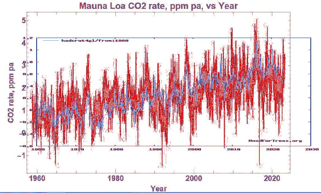
Fig. 5 - Growth of anomalous temperatures (blue) since 1960 (HADCRUT4gl 2022) vs growth rate of atmospheric CO2 concentration (NOAA 2024) (red)

Fig. 6 - Cross-correlation of the rate of increase in anomalous temperatures since 1960 (HadCRUT4gl 2022) and the rate of increase in atmospheric CO2 concentration (NOAA 2024) with zero time lag.

If we take the Mauna Loa annual CO2 concentration increase rate data (NOAA 2024) and correlate it with the anomalous temperature increase rates (HadCRUT4gl 2022) between 1960 and 2022, we find that there is no correlation and R=0.068, or R2 = 0,0046, see Figure 6. Thus, statistically we can reject the IPCC hypothesis due to the zero time delay between the two series. However, if we analyse the correlation coefficient as a function of the time lag between the two series, we find that the largest correlation coefficient R=0.26 is if we delay the time series of the rate of increase in CO2 concentration at Mauna Loa by 6-8 months compared to the time series of the rate of increase in global anomalous temperatures. Thus, we can clearly conclude that we can reject the IPCC hypothesis, and what is more, it cannot be true that the evolution of atmospheric CO2 concentrations determines the evolution of global temperatures because it is delayed by several months in the annual cycle behind the temperatures.

5. Conclusions

In conclusion, it is statistically impossible to reject M. Salby's hypothesis that global ocean temperature controls atmospheric CO2 concentration. Since the CO2 concentration itself should theoretically be proportional to the time integral of anomalous temperatures, this integration delay in the annual cycle of 6-8 months is observed in the 1960-2022 data, by which the increase/decrease in CO2 concentration is delayed behind the increase/decrease in temperature.

On the other hand, the IPCC hypothesis that changes in atmospheric CO2 concentration cause changes in global temperatures can be clearly rejected. There is no statistically significant correlation between these series (R=0.07). Moreover, there is a higher correlation between these series when the CO2 concentration growth rate series is delayed by 6-8 months compared to the temperature growth rate series.

Guest-Editor: Stein Storlie

Bergsmark

References

Henry, W. (1803): Henry’s law.

Jouzel J., C. Waelbroeck, B. Malaizé, M. Bender, J.-R. Petit, N.I. Barkov, J.-M. Barnola, T. King, V.M. Kotlyakov, V. Lipenkov, C. Lorius, D. Raynaud, C. Ritz, T. Sowers (1996): Climatic interpretation of the recently extended Vostok ice records. Climate Dynamics, Vol. 12, 513 – 521.

Legrand M., C. Lorius, N.I. Barkov, V.N. Petrov (1988): Vostok (Antarctica) ice core: atmospheric chemistry changes over the last climatic cycle (160,000 years). Atmospheric Environment, Vol. 22, No. 2, 317-331.

Petit, J.-R., J. Jouzel, D. Raynaud, N.I. Barkov, J.-M. Barnola, I. Basile, M. Bender, J. Chappellaz, M. Davis, G. Delaygue, M. Delmotte, V.M. Kotlyakov, M. Legrand, V. Lipenkov, C. Lorius, L. Pépin, C. Ritz, E. Saltzman, and M. Stievenard (1999): Climate and Atmospheric History of the Past 420,000 years from the Vostok Ice Core, Antarctica. Nature, 399, 429–436.

Salby, M. (2011): Sydney - Global Emission of Carbon Dioxide: The Contribution from Natural Sources" https://www.youtube.com/watch?v=YrI03ts 9I

Salby, M. (2015): London - Climate Scientist Murry Salby Returns! - Presents NEW SCIENCE https://www.youtube.com/watch?v=rCya4LilBZ8

Salby, M. (2016): London - Atmospheric Carbon, 18 July 2016, University College London https://www.youtube.com/watch?v=sGZqWMEpyUM https://www.youtube.com/watch?v=O8niiyDn2FI&pp=ygUPTXVycnkgU2FsY nkgQ08y short - https://www.youtube.com/watch?v=J2YQanhRDOQ

Salby, M. (2011): Sydney - Global Emission of Carbon Dioxide: The Contribution from Natural Sources" https://www.youtube.com/watch?v=YrI03ts 9I

Salby, M. (2015): London - Climate Scientist Murry Salby Returns! - Presents NEW SCIENCE https://www.youtube.com/watch?v=rCya4LilBZ8

Salby, M. (2016): London - Atmospheric Carbon, 18 July 2016, University College London https://www.youtube.com/watch?v=sGZqWMEpyUM https://www.youtube.com/watch?v=O8niiyDn2FI&pp=ygUPTXVycnkgU2FsY nkgQ08y short - https://www.youtube.com/watch?v=J2YQanhRDOQ

Salby, M. (2015): Essen - Neue Forschungsergebnisse zum Ursprung atmosphärischen CO2 https://www.youtube.com/watch?v=HPkkSN82KMY

Salby, M. (2018): Hamburg - What is Really Behind the Increase of Atmospheric CO2? https://www.youtube.com/watch?v=b1cGqL9y548

On-line data

HADCRUT4 (2023): Temperature -

Science of Climate Change

https://scienceofclimatechange.org

https://www.woodfortrees.org/plot/hadcrut4gl/from:1960 Derivative of temperature - https://www.woodfortrees.org/plot/hadcrut4gl/from:1960/derivative

NOAA (2024): Trends in atmospheric carbon dioxide [cit. 19.05.2024]. Dostupné z: https://gml.noaa.gov/ccgg/trends/

Petit, J.-R.; Jouzel, J.; Raynaud, D.; Barkov, N.I.; Barnola, J.-M.; Basile, I.; Bender, M.L.; Chappellaz, J.A.; Davis, M.D.; Delaygue, G.; Delmotte, M.; Kotlyakov, V.M.; Legrand, M.; Lipenkov, V.Y.; Lorius, C.; Pépin, L.; Ritz, C.; Saltzman, E.S.; Stievenard, M. (2001-11-01): NOAA/WDS Paleoclimatology - Vostok - Isotope and Gas Data and Temperature Reconstruction. [indicate subset used]. NOAA National Centers for Environmental Information. https://doi.org/10.25921/kcry-ae86. Accessed [date]: https://www.ncei.noaa.gov/access/metadata/landing-page/bin/iso?id=noaaicecore-2453

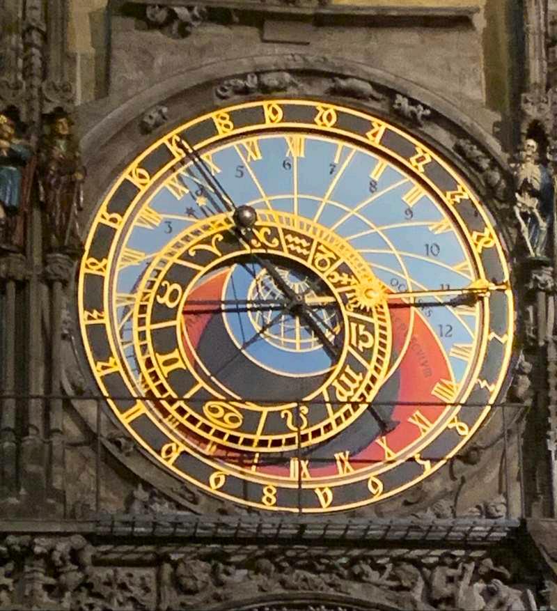
Science of Climate Change

https://scienceofclimatechange.org

The Astronomical clock in Prague at the time of the Conference. Photo: J.-E. Solheim

Klimarealistene

Vollsveien 109

1358 Jar, Norway

ISSN: 2703-9072

Correspondence:

dk@itia.ntua.gr

Vol. 4.3 (2024)

pp. 39 – 49

The Relationship between Atmospheric Temperature and Carbon Dioxide Concentration

Demetris Koutsoyiannis

Department of Water Resources and Environmental Engineering, School of Civil Engineering, National Technical University of Athens, Zographou, Greece

Abstract

Human-produced CO₂ by fossil fuel combustion, combined with the rising atmospheric CO₂ concentration and the observed temperature increase, enabled a compelling narrative to be constructed, in which these three facts, in that order, formed a chain of causality. The narrative has been embraced by global political elites to promote their interests. It has also become dominant in public perception, by means of issuing threats for all aspects of life due to alleged climate impacts. My recent work has challenged the alleged causal relationships that form the narrative. A stochastic method for detecting causality showed that temperature change can potentially cause changes in CO₂ concentration, but not vice versa. Temperature increase causes the biosphere to expand and, in turn, produce more naturally emitted CO₂, which accounts for 96% of total emissions. All relevant data sets confirm these findings. In particular, instrumental and proxy data support the natural origin of the change in the isotopic composition of atmospheric CO₂, and century-long longwave radiation data show no discernible effect of increased CO₂ concentration on the greenhouse effect

Keywords: Causality; stochastics; greenhouse effect; longwave radiation; water vapour; carbon dioxide

Submitted 2024-11-19, Accepted 2024-11-24. https://doi.org/10.53234/scc202412/15

(What’s the need for physics / The laws don’t count / In a metaphysical phase / The passions rule) Lavrentis Machairitsas, from the lyrics of «Πεθαίνω

1. Introduction

(“Dying for you”)

Powerful elites, assuming the role of the planet saviours, blame human CO₂ emissions for every evil that befalls the Earth. In this, they are assisted by so-called climate science, which has constructed the causal chain, “a”, “b”, “c”, shown in Figure 1 (upper row) as its core. Not only is this chain promoted by IPCC and the political and economic interests, but is also supported by mainstream “sceptics”. However, in my view, it is naïve, as climate is too complex to be represented in such a simplistic sequence with a single cause. Besides, the causality direction is mostly opposite to the prevailing assumption and is represented by the lower row in Figure 1, which is a result of my recent research publications that are summarised below. In particular, causal links “b” and “c”arereplacedby“β”and“α”,respectively,whichhaveoppositedirection,while“a”isofminor importance as other factors trump it. These are examined in the next sections of this paper.

2. Assumed causal link “a”: Is the increase in atmospheric CO₂ caused by human emissions?

One of the arguments in support of the popular affirmative reply to the above question has been the decrease of the abundance of the ¹³C isotope, represented by the standard metric δ¹³C, in the atmosphere, which has been attributed to the burning of fossil fuels, and has been known as the Suess (1955) effect. Indeed, the time series of the atmospheric δ¹³C, seen in the lower graph of

Figure 2, shows a decreasing trend

Mainstreambut implausible causal chain (for the kindergarten):

Climate (i.e. human CO₂) impacts on everything*

*from hydrology to kidney stones

Proposed causal chain (for adults):

Hydrology and other climate drivers**

**kidney stones excluded

Figure 1: Graphical depiction of the subject of this paper, with the upper row of arrows showing the mainstream causal chain that is popular among climate zealots and mainstream climate sceptics, and the lower row showing the proposed alternative based on my recent publications. The smaller arrow for the human CO₂ emissions in the lower row corresponds to the fact that they only contribute 17% to the increase of [CO₂] (causal link “a΄”), while natural emissions by the expanded biosphere due to increased T contribute 83% (causal link “β”; see Section 2). The footnotes are included for illustration and are documented as follows: A Google Scholar search for the terms "climate impacts" and "hydrology" yields 34 200 publications1 and a search for the terms "climate change" and "kidney stones" yields 3710 publications2 .

Diagnostic results at Mauna Loa, Hawaii: Increasing (rather than decreasing) net input isotopic signature

Explained variance: 99%

Modelling results at Barrow,Alaska: Perfect model performance by considering nothing more than natural seasonality

Figure 2: Reproduction of the graphical abstract of Koutsoyiannis (2024a).

1 https://scholar.google.com/scholar?q=%22climate+impacts%22+%22hydrology%22

2 https://scholar.google.com/scholar?q=%22climate+change%22+%22kidney+stones%22

However, as shown in the study by Koutsoyiannis (2024a), which fully reproduced the observations with a simple model (lower graph of Figure 2), the net input signal of the atmospheric, δ¹³CI, is not decreasing in some cases, it is increasing (upper graph of Figure 2). A constant δ¹³CI of slightly less than –13‰ at an overannual time scale is representative across the entire globe for the entire period of measurements. The same value holds for the entire period after the Little Ice Age, as confirmed by proxy data These results support the conclusion that natural causes drove the increase of CO₂ concentration ([CO₂]). A human-caused signature (Suess effect) is non-discernible.

Besides, while fossil fuels have indeed a small δ¹³C signature, down to –26‰, and hence their input δ¹³CI is low, C3 plants (e.g., evergreen trees, deciduous trees and weedy plants) have much lower δ¹³C values than fossil fuels, down to –34‰, and thus their input δ¹³CI is even lower (Koutsoyiannis, 2024b) Lower values than in fossil fuels, also appear in other CO₂ sources. When the C3 plants (and many other organisms) respire, they emit to the atmosphere low δ¹³CI, decreasing the atmospheric δ¹³C content. It is therefore absurd to suggest that it is the emission from burning fossil fuels (4% of the total) that causes the atmospheric δ¹³C value to fall.

A more detailed account of the atmospheric CO₂ balance was presented by Koutsoyiannis (2024c). That study fully overturned the IPCC’s weird claims of different behaviour of the anthropogenic from the natural CO₂, where the former allegedly has a multi-millennial lifetime in the atmosphere. Contrary to this, Koutsoyiannis (2024c), showed that the CO₂ mean residence time in the atmosphere is: (a) independent of the origin (human or natural), (a) about 4 years on overannual basis, and (c) seasonally varying with lowest value < 2 years (see Figure 3, upper right).

Meanresidencetime (W): 3.9 years (seasonal variation: 1.6 – 9.9 years).

Netinflowseasonalvariationrange: 130 ppm/year in 1960s; 240 ppm/year now (biosphere expansion comparewith human emissionsof max 5 ppm/year).

Modelperformance:excellent.

The samestudy highlightedthefactthat since the 1960sthe biosphere hassubstantiallyexpanded, as seen from the observations of net natural inflow of CO₂ (see Figure 3, upper left). The expansion was caused by the increase of temperature. Indeed, living organisms love warm conditions and increase their respiration R with temperature T exponentially, following the empirically proved relationship, known as the Q10 model (Patel et al., 2022):

Figure 3: Reproduction of the graphical abstract of Koutsoyiannis (2024c).

where ��10 is a dimensionless parameter and ��0 and ��(��0) are reference values From the model results, we infer that the biosphere expansion from 1958 to 2023 resulted in an upsurge, Δ(EN), of the natural emission, EN, equal to 26.1 ppm CO₂/year For comparison, the human emissions in this period varied from 2.1 to 5.4 ppm CO₂/year at the beginning and end of this period, respectively. The related time series are seen in Figure 4. From the entire figure, it can be inferred that the standard practice of both IPCC and mainstream sceptics to focus on the lower part of the graph (the two curves below 10 ppm/year in Figure 4) is inappropriate as it misses the “forest”, i.e.,theentirebiosphere. ThisIPCC’s practiceisreflectedinthefollowingquotation (IPCC,2021, p. 54): “Emissions from natural sources, such as the ocean and the land biosphere, are usually assumed to be constant, or to evolve in response to changes in anthropogenic forcings or to projected climate change.” The inappropriateness of this practice can be inferred from the facts that the biosphere: (a) has its own dynamics that is not governed by human emissions, and (b) quantitatively has 25 times higher contribution than human emissions, even according to IPCC estimates (see Figure 5). If more recent estimates are considered, the human contribution becomes even less important. Specifically, in the recent publication by Lai et al. (2024) the estimates of gross photosynthesis and respiration are higher than the IPCC’s, namely 157 and 149 Gt C/year, respectively (instead of the IPCC’s estimates of 142.0 and 136.7 Gt C/year, shown in Figure 5).

Biosphere expansion

EN: emissions, natural EH: emissions, human SN: sinks, natural Balance (atmpospheric storage)

2.1

5.4

2.2

Figure 4: CO₂ fluxes in the atmosphere for the period 1958-2023, as inferred by human emission estimates, CO₂ concentration data, and the model by Koutsoyiannis (2024c) (for EN and SN).

84.5 2023, 110.5

Preindustrial Modern additions

Terrestrial Maritime Human

Gross photosynthesis

Total respiration and fire

Volcanism, freshwater outgassing

Absorption and photosynthesis

Rock weathering Respiration

Fossil fuel and cement production

Land use change

Ouflows: –221.8 Inflows: 226.9 (Balance: 5.1)

CO₂ flux (Gt C / year)

Figure 5: “Official” IPCC’s (2021; Fig. 5.12) estimates of CO₂ fluxes, in an “unofficial” presentation adapted from Koutsoyiannis (2024c).

Even keeping the IPCC’s estimates shown in Figure 5, we can make the following observations that are in line with the proposed interpretation of CO₂ fluxes:

1. Humans are responsible for only 4% of carbon emissions.

2. The vast majority of changes in the atmosphere since 1750 (red bars in the graph) are due to natural processes, respiration and photosynthesis.

3. The increases in both CO₂ emissions and sinks are due to the temperature increase, which expands the biosphere and makes it more productive.

4. The terrestrial biosphere processes are much more powerful than the maritime ones in terms of CO₂ production and absorption.

5. The increase of natural CO₂ emissions by the ocean biosphere alone is much larger than human emissions.

6. The modern (post-1750) CO₂ additions to pre-industrial quantities (red bars in the right half of the graph) exceed the human emissions by a factor of ~4.5.

Furthermore, by combining Figure 4 and Figure 5 we can see that the vast majority of the [CO₂] increase in 2023 is due to the increased natural emissions. Namely, the percentage from this increasefor2023is26.1 / (26.1+5.4)=83%,leaving17%tohumanemissions(cf.captionof Figure 1 and also Koutsoyiannis, 2024f, section 5.3).

3. Assumed causal link “b”: Does the increase in atmospheric CO₂ cause temperature increase?

An initial investigation of the potential causality in atmospheric [CO₂] and temperature based on observations, rather than models, was undertaken by Koutsoyiannis and Kundzewicz (2020), prompted by the fact that the increasing pattern of atmospheric CO₂ concentration remained unaffected by the decrease of human CO₂ emissions due to the covid lockdowns. It was followed by the development of a new stochastic method by Koutsoyiannis et al. (2022a,b). This began with a review of approaches to causality over the entire knowledge tree, from philosophy to science and to technological and socio-political application, and identified the major unresolved problems. The developed methodologyposited amodest objective: Todetermine necessaryconditions that are operationally useful in identifying or falsifying causality claims; sufficient conditions were not sought. The necessary conditions are important in two respects:

• In a deductive setting, to falsify a hypothesized causality relationship by showing that it violates a necessary condition.

• In an inductive setting, to add evidence in favour of the plausibility of a causality hypothesis.

The methodology replaced events with stochastic processes. It is fully based on stochastics a superset of probability and statistics, with time playing an essential role. Specifically, it is based on a reconsideration of the concept of the impulse response function (IRF). Real-world data, namely time series of observations, constitute the only basis of the method application Model results and so-called in silico experimentation are categorically excluded. On the contrary, the method provides a test bed to identify whether or not models are consistent with reality.

The general setting of the method is for the Hen-Or-Egg case, i.e., bidirectional causality, while the unidirectional cases of a causal system (causality direction according to the hypothesis) or an anticausal system (causality direction opposite to the hypothesis) are derived as special cases.

The method was formulated as a general stochastic method, while a more extensive analysis of theclimate-relatedcausality chainswas madeinafollow-up paper byKoutsoyianniset al. (2023), which extended the approach to multiple scales and applied it to the longest period covered by instrumental data. Subsequently,Koutsoyiannis (2024d)further refinedthe methodologyand also used proxy data covering the entire Phanerozoic.

The results have always been the same: The common perception that increasing [CO₂] causes increased T can be excluded as it violates the necessary condition for this causality direction. In contrast, the causality direction T → [CO₂] is plausible. An illustration of such results is provided in Figure 6, where the fact that [CO₂] changes follow those in T is evident even visually. The graph uses a lag of 6 months (0.5 years) for illustration. Detailed application of the stochastic method results in a median and mean time lag slightly higher, 0.6 and 0.7 years, respectively, as shown in Figure 7. This is for an annual time scale of analysis and for the instrumental data. If we consider a decadal time scale for the same data, the causality direction remains the same and the lagsincrease to 3.2 and 3.3 years, respectively. If we use proxy data for time scales up to a million years, again the causality direction is the same (the time lags are positive) as seen in Figure 7

Figure 6: Reproduction of the graphical abstract of Koutsoyiannis et al. (2023), showing different plots of the annual averages of differenced time series of temperature (ΔT) and the logarithm of [CO₂] (Δln[CO₂]) for a differencing time step of one year and a lag of six months On the left graph, each point represents the time average for a duration of one year ending at the time of its abscissa.

Figure 7: Summary of time lags (in years) of the T → [CO₂] potentially causal relationship (positive in all cases, meaning that [CO₂] change lags behind T change); h1/2 and μh denote the median and mean time lag, respectively.

4. Assumed causal link “c”: Are there climate impacts, or ultimately, do human CO₂ emissions affect everything?

While “climate science” babbles on about CO₂ as the determinant greenhouse gas (calling it the “principal control knob”), hydrology has routinely quantified the greenhouse effect for 70 years. This is necessary in evaporation calculations and the related formulae are based on data of atmospheric moisture. Koutsoyiannis and Vournas (2023) used a century-long collection of data on downwelling longwave radiation at the ground level The analysis of this data set showed that there is no discernible effect on the greenhouse effect intensity, despite the increase of atmospheric [CO₂] from 300 to >400 ppm in a century (see Figure 8)

Calculated by Brutsaert's formula (W/m²)

2012-13 / Li et al.

2007-10 / Carmona et al.

1973-74 / Aase & Idso

1961-62 / Swinbank

1955 / Stoll & Hardy (from Satterlund)

1926 / Robitzsch (from Brunt and Pekeris )

1922-26 / Dines (from Brunt and Swinbank)

1912 / Ångström

Equality line

Linear (2007-10 / Carmona et al.)

Linear (1973-74 / Aase & Idso)

Nonnegligible amplification of the greenhouse effect, due to increase of CO₂ concentration from 300 to >400 ppm in a century, would be seen as a systematic gradual displacement of the points to the right for the more recent series of observations.

Is there any sign of such displacement?

Measured (W/m²)

Figure 8: Reproduction (with kind permission of IAHS) of Figure 2 from Koutsoyiannis and Vournas (2023; after adaptation) showing plots of downward radiation of the atmosphere, measured vs. calculated (by the Brutsaert’s, 1975, formula, which accounts for water vapour pressure only), in eight data sets used in the study. For the two data sets with the largest number of points, the linear regression lines are also shown, along with their equations.

Explanation of this result and quantification of relevant importance of greenhouse drivers were performed by the follow-up study by Koutsoyiannis (2024e). This was based on the standard theory and an established model of radiation in the atmosphere (MODTRAN), as well as on satellite radiation data. Using MODTRAN results and data from NASA’s ongoing project Clouds and the Earth’s Radiant Energy System (CERES, 2021), the study constructed a macroscopic relationship for longwave radiation, i.e.:

where ��D,O denotes the downwelling (D) and outgoing (O) longwave radiation flux; �� is the temperature near the ground level; ��a is the water vapour pressure near the ground level; [CO2] is the atmospheric CO2 concentration with a reference value [CO2]0 = 400 ppm; �� is the cloud area fraction; ��∗ , ��∗ , ��

are dimensional parameters, with units [L

and [

], respectively; and ����, ����, ��CO₂, ���� are dimensionless parameters. The parameter values were optimized based on clearsky MODTRAN results, except ����, which was estimated from CERES satellite data.

This relationship was applied to find the relative importance of each of the factors ���� ∈ {��,��a,[CO2],��} on the longwave radiation by means of the total differential:

denotes the log-log derivative, i.e. (Koutsoyiannis, 2023):

The importance of other greenhouse gases was also assessed by direct numerical evaluation with MODTRAN. The final results are depicted in Figure 9. The chart on the left explains the findings of the study by Koutsoyiannis and Vournas (2023): given that the contribution of CO₂ is only 4% there could be no discernible effect of the [CO₂] increase in a century on the downwelling longwave (LW) radiation. The chart on the right suggests that the same should have been the case (macroscopically) with the outgoing LW radiation if data of similar length existed.

CONTRIBUTION OF THE GREENHOUSE DRIVERS TO THE LW RADIATION FLUXES

All evidence suggests that the recent increase in atmospheric temperature was not caused by the [CO₂] increase. The question of what might have caused it is not easy to answer as numerous factors influence climate, both internal and external to the climatic system. Before trying to answer it, one would think of additional questions such as:

1. Do complex dynamical systems need external agents to change their state?

2. Should we expect the temperature to be stable?

3. What caused a cause?

4. Have the huge changes in global temperature during the Phanerozoic been explained?

None of these additional questions has an affirmative answer. In particular, the negative answer to question 1 has been extensively studied in Koutsoyiannis (2006, 2010, 2013).

Nevertheless, Koutsoyiannis et al. (2023) examined some possible mechanisms internal to the climatic system, namely albedo, ENSO and ocean heat,in which the change was found to precede that of temperature (and a fortiori of CO₂). The change of the albedo based on CERES data is shown in Figure 10 (left). A decline of the albedo of about 0.004 is seen for the entire observation

Figure 9: Reproduction of Figure 24 from Koutsoyiannis (2024e) showing the contribution of the greenhouse drivers to the LW radiation fluxes

period, which translates to 1.4 W/m2. This is much greater than the average imbalance (net absorbed energy) of the Earth, which, if calculated from the ocean heat content data, is about 0.4 W/m2 (Koutsoyiannis, 2021).

Apparently, the albedo decline has no relationship with the increase of [CO₂]. Rather it has been caused by (or at least it is consistent with) a decline in cloud area fraction, also seen in Figure 10 (right) Notably, this explanation does not enable predictability of future climate. Rather, it raises additional questions, e.g., what caused the decline in clouds? Yet it highlights the importance of H₂O and the insignificance of CO₂ in climate

Figure 10: (left) Top-of-atmosphere albedo time series (continuous line) from NASA’s CERES data set, along with linear trend (dashed line); source Koutsoyiannis et al. (2023). (right) Total cloud area fraction (single lines) from NASA’s CERES data set, along with linear trends (double lines); source Koutsoyiannis and Vournas (2024) (with kind permission of IAHS)

5. Concluding remarks

• The foundation of the modern climate edifice is afflicted by erroneous assumptions and speculations.

• The causal chain promoted by mainstream science is naïve and wrong.

• In scientific terms, the case of the magnified importance of CO₂, the focus on human emissions thereof, and the neglect of the ~25 times greater natural CO₂ emissions constitute a historical accident.

• This accident was exploited in non-scientific (politico-economic) terms.

• For complex systems, observational data are the only scientific test bed for making hypotheses and assessing their validity.

• The real-world data do not agree with the “mainstream science” (a euphemism for sophistry).

• The results I have presentedare scientific and thereforemay not berelevant to the climate narrative, which has a non-scientific aim.

Guest Editor: Stein Storlie Bergsmark

References

Brutsaert W, 1975: On a derivable formula for long-wave radiation from clear skies, Water Resour. Res., 11, 742–744

CERES, 2021: CERES_SSF1deg_Hour/Day/Month_Ed4A Data Quality Summary, Version 2. https://ceres.larc.nasa.gov/documents/DQ_summaries/CERES_SSF1deg_Ed4A_DQS.pdf (Updated 8/4/2023; accessed 15 February 2024).

https://scienceofclimatechange.org

IPCC (Intergovernmental Panel on Climate Change), 2021: Climate Change 2021: The Physical Science Basis. Contribution of Working Group I to the Sixth Assessment Report (AR6) of the Intergovernmental Panel on Climate Change; ed. by Masson-Delmotte, V., Zhai, P., Pirani, A., Connors, S.L., Péan, C., Berger, S., Caud, doi: 10.1017/9781009157896.

Koutsoyiannis D, 2006: A toy model of climatic variability with scaling behaviour, Journal of Hydrology, 322, 25–48, doi: 10.1016/j.jhydrol.2005.02.030.

Koutsoyiannis D, 2010: A random walk on water, Hydrology and Earth System Sciences, 14, 585–601, doi: 10.5194/hess-14-585-2010.

Koutsoyiannis D, 2013: Hydrology and Change, Hydrological Sciences Journal, 58 (6), 1177–1197, doi: 10.1080/02626667.2013.804626.

Koutsoyiannis D, 2021: Rethinking climate, climate change, and their relationship with water, Water, 13, 849, doi: 10.3390/w13060849.

Koutsoyiannis D, 2023: Stochastics of Hydroclimatic Extremes – A Cool Look at Risk, Edition 3, Kallipos Open Academic Editions, Athens, 391 pp, doi: 10.57713/kallipos-1

KoutsoyiannisD,2024a: Net isotopic signature of atmospheric CO₂ sources and sinks: No change since the Little Ice Age, Sci, 6 (1), 17, doi: 10.3390/sci6010017.

Koutsoyiannis D, 2024b: Definite change since the formation of the Earth [Reply to Kleber, A. Comment on “Koutsoyiannis, D. Net isotopic signature of atmospheric CO2 sources and sinks: No change since the Little Ice Age. Sci 2024, 6, 17”], Sci, 6 (4), 63, doi:10.3390/sci6040063.

Koutsoyiannis D, 2024c: Refined reservoir routing (RRR) and its application to atmospheric carbon dioxide balance, Water, 16 (17), 2402, doi: 10.3390/w16172402.

Koutsoyiannis D, 2024d: Stochastic assessment of temperature – CO₂ causal relationship in climate from the Phanerozoic through modern times, Mathematical Biosciences and Engineering, 21 (7), 6560–6602, doi: 10.3934/mbe.2024287.

Koutsoyiannis D 2024e: Relative importance of carbon dioxide and water in the greenhouse effect: Does the tail wag the dog?, Science of Climate Change, 4 (2), 36–78, doi: 10.53234/scc202411/01.

Koutsoyiannis D, 2024f: The superiority of refined reservoir routing (RRR) in modelling atmospheric carbon dioxide, ResearchGate, doi: 10.13140/RG.2.2.32285.32489

Koutsoyiannis D, Kundzewicz ZW, 2020: Atmospheric temperature and CO₂: Hen-or-egg causality?, Sci, 2, 72, doi:10.3390/sci2040077

Koutsoyiannis D, Onof C, Christofides A, Kundzewicz ZW, 2022a: Revisiting causality using stochastics: 1. Theory, Proc. R. Soc. A, 478, 20210835, doi: 10.1098/rspa.2021.0835.

Koutsoyiannis D, Onof C, Christofides A, Kundzewicz ZW, 2022b: Revisiting causality using stochastics: 2. Applications, Proc. R. Soc. A, 478, 20210836, doi: 10.1098/rspa.2021.0836.

Koutsoyiannis D, Onof C, Kundzewicz ZW, Christofides A, 2023: On hens, eggs, temperatures and CO2: Causal links in earth’s atmosphere, Sci, 5, 35, doi:10.3390/sci5030035

Koutsoyiannis D., Vournas C, 2024: Revisiting the greenhouse effect a hydrological perspective, Hydrol. Sci. J., 69, 151–164, doi: 10.1080/02626667.2023.2287047.

Lai J, Kooijmans LM, Sun W, Lombardozzi D, Campbell JE, Gu L, Luo Y, Kuai L, Sun Y, 2024: Terrestrial photosynthesis inferred from plant carbonyl sulfide uptake, Nature, 634, 855–861.

Patel KF, Bond-Lamberty B, Jian JL, Morris KA, McKever SA, Norris CG, Zheng J, Bailey VL, 2022: Carbon flux estimates are sensitive to data source: A comparison of field and lab temperature sensitivity data, Environ. Res. Lett., 17, 113003.

Suess HE, 1955: Radiocarbon concentration in modern wood. Science, 122, 415–417.

https://scienceofclimatechange.org

Klimarealistene

Michelets vei 8 B 1366 Lysaker, Norway

ISSN: 2703-9072

Correspondence: j.croll@ucl.ac.uk

Vol. 4.3 (2024)

pp. 50-63

Does the Geological Evidence indicate a Causal Link between CO2 and Climate Change?

James Croll

Emeritus Professor of Civil Engineering University College London

Abstract

Climate is changing and always has with many and varied recognised drivers. Earth‘s interaction with our celestial neighbours within the solar system and the solar systems relationships within the galaxy being perhaps the most recognised and important of these primary drivers of climate change at virtually all time scales. On the other hand, GHGs and especially CO2 are recognised as primary factors in making Earth habitable and providing the fundamental requirements for the evolution of both faunal and floral life. So why is CO2 attracting such opprobrium and is there any rationale for the current, single minded, global quest to reduce its levels?

The following will examine some of the evidence from the geological records addressing this issue. It will attempt to show how many fundamental geological processes may have at least part of their explanation in terms of Earth’s changing climate. And it will also try to demonstrate that over most of the past 600 Ma there has been very little evidence of a direct link between CO2 and climatic conditions. In addition, it will suggest there is no definitive evidence as to whether CO2 or climate is responsible for ensuring their close correlation over the past 60 Ma. But the consideration that there are well recognised and scientifically sound explanations for observed cyclic changes in climate, especially over the past 6 Ma, and again rational scientific processes that account for CO2 following these climate cycles, should surely tip the balance of probability towards climate change being the primary driver of CO2

Keywords: Climate change; causal link; CO2, temperature, phanerozoic eon; cenozoic era

Submitted 2024-11-20, Accepted 2024-11-24. https://doi.org/10.53234/scc202412/16

1. Introduction

Over widely varying time periods, Earth’s temperature experiences major cycles driven by the interaction with our celestial neighbours. Our daily interaction with the Sun, resulting from Earth’s rotation about its own axis, causes considerable day and night temperature variations. These circadian temperature cycles are of similar orders of magnitude to those experienced through seasonal variations resulting from Earth’s axis of tilt relative to the plane of its orbit about the Sun. The temporal variations in the tilt axis and its precession over time periods measured in 10s to 100s ky, interacting with the changing eccentricity of Earth‘s solar orbit, are in turn now generally accepted as being responsible for the temperature changes accompanying the periodic glacials and interglacials occurring when Earth is experiencing icehouse climate conditions. And the icehouse and

Science of Climate Change

https://scienceofclimatechange.org

hothouse climate periods, having periodicities measured in 10s to 100s My, are believed to at least be partially caused by the variations in the cosmic ray flux (CRF) resulting from the motions of our solar system within and normal to the galactic plane.

These first order extraterrestrial drivers of climate, for which we homo sapiens have no control, are clearly modified by other factors, over which there are some we have limited control, but mostly we don‘t. And of course the particular modifying factor upon which the globe is currently focussed is that of the influence of greenhouse gases (GHG) and in particular whether post-industrial anthropogenic increases in CO2 have been responsible for recently recorded climate changes. The following contribution will focus upon what the geological evidence tells us about the potential importance of CO2 as a determinant of climate change.

But before concentrating on the geological perspective as to whether GHGs might have had an impact on climate, it is perhaps worth pausing to acknowledge just how fortunate we are to be living on a planet for which natural processes have provided an atmosphere containing these GHGs. As will be shown, the GHGs over much of the past 600 Ma have been at levels that mean, in contrast with other planets in the solar system, our planet is not perpetually frozen. And despite being far more than levels in our current atmosphere over most of this past 600 Ma, the rich faunal and floral life we currently enjoy was able to emerge. It is therefore no exaggeration to claim that without GHGs, and especially H2O and CO2, our planet would be lifeless. So, with both H2O and CO2, such vital gases of life, the only issue of current concern is whether the changes in the levels of these recognised GHGs, being produced by human activities that are releasing some of the carbon locked into ancient sediments, are actually upsetting the balance of the natural processes. As will be shown, the evidence from the geological records strongly suggest they are not.

2.The Phanerozoic eon

Because there was such a rich and rapidly developing range of living species over the past 600 Ma, the fossil record buried within the sediments provides a rich resource for understanding how climate has changed and what has been the nature of the atmospheric composition during these changes.

2.1 Climate and CO2

Over the Phanerozoic eon (the past 540 Ma), proxies of atmospheric CO2 have shown levels that for most of this period have been 10 to 20 times current concentrations and yet this same period witnessed an explosion of both faunal and floral life. However, over most of this period proxies of ocean temperatures, determined from exhaustive measurement of fossilised calcitic shells, display very poor correlation with these CO2 levels. For example, while CO2 levels were at temporal highs around the late Ordovician (-450 Ma) and Jurassic (-160 Ma) periods, Earth was actually experiencing icehouse climate conditions. This can be seen in Fig 1. The upper blue curve provides a measure of the CO2 levels as reported by Berner16. To convert the log scale to absolute values of CO2 the value of around 1.5 during the Ordovician period translates as 5000ppm – more than 10 times those currently in the atmosphere. During the early part of the Cambrian period the levels reached as high as 7000ppm. This compares with the approx. 420ppm today.

Fig 1 Shows the levels (top blue curve) and sea temperatures (various lower curves) over the Phanerozoic eon. Ice house periods marked by the blue bars at the top. To convert left scale to temperatures and right scale to CO

The lower group of curves of Fig 1 plot proxies of ocean temperature, subject to various levels of filtering of the data taken from the measurements of oxygen isotopes in calcite shells, reported by Veitzer at the left scale, a value of C (see also Fig 2). What Fig 1 demonstrates very clearly is the lack of correlation between CO and ocean temperatures over almost the entire period of the Phanerozoic. It also shows the clear cyclic nature of the climate over this 540 Ma again showing little relationship with the CO trend. Concentrating on the lower black curve, for which the data points at 10Ma intervals are as plotted as running averages ervals of 50Ma, the 3 full climate cycles between say periodicity of around 130Ma. We will return to the significance of this climate periodicity in later discussion.

2.2 Climate and the Fossil Record

One of the notable achievements of the painstaking geological research over the past 250 years, since the contributions of Hutton4, has been the identification of distinct geological periods having dominant time periods of around 60 Ma. Boundaries between these geological periods have been defined from observations, generally over widely dispersed spatial domains, of major discontinuities in the nature of the fossil records. When compared with the patterns of ocean temperature derived from the isotope analysis of marine calcitic fossils, it becomes clear that most of these period boundaries coincide with times at which Earth climate is experiencing extreme levels or major and rapid climate change. This is illustrated in Fig 2. That species might find it difficult to adapt to sudden changes or extremes of temperature is perhaps as would be expected. But in relation to our present discussion, it does underline the cyclic nature of climate over the past 540Ma. A pattern

that is certainly not reflected in the CO2 records shown in Fig 1.

Fig 2 Climate cycles over the Phanerozoic (with cold icehouse conditions above!) showing how the majority of the geological period boundaries coincide with times at which Earth climate is undergoing rapid and extensive climate change or experiencing extremes in hot or cold climate.

It is of related significance that in many cases these periods of massive and sudden climate change correspond with times at which mass extinctions occur. The recorded levels of mass extinction are shown in Fig 317. These blue bars record the percentages of marine genera that became extinct over the period of time indicated by the widths of the respective blue bars.

3 Shows the percentage of marine genera that become extinct in the time period represented by the widths of the vertical blue bars and their relationship with the boundaries between geological periods and by extension climate cycles

Fig

2.3 Possible Causations for Climate Cycles

There is no universal agreement on what has caused these cycles of climate over the Phanerozoic eon. From the above it is clear it is not CO2. Perhaps the most convincing explanation is that related to the intensity of the cosmic ray flux (CRF) experienced by the solar system. This has been discussed by many but one of the most comprehensive discussions of the science underpinning CRFs impact on climate is that of Shaviv9. Quite independent of the work of Veizer, this study of the CRF revealed in meteorite evidence has been found to produce temperature predictions, based upon the cyclic pattern of the CRF data, that almost overlays the temperature proxies from the study of calcitic shell fossils8. This is shown in Fig 6 where the black, filtered, plot of oxygen isotope proxies of ocean temperature8,9 shown by the broken curve is closely related to the predictions based upon CRF shown by the full black cycles. On the reasonable surmise that changes in calcitic shell fossils are not driving the motions of our solar system through and about the galactic plane, considered to be the explanation for the cycle patterns of CRF variation, it seems reasonable to assume that at least a major contribution to Phanerozoic climate derives from variations in CRF.

2.4 Climate and Tectonics

There are of course other reasons why the geological records of fossils undergo sudden breaks. It has been extensively documented that the sedimentary record shows well defined discontinuities at which there are missing times between adjacent layers of sediments. Often, these „unconformities “have been shown to display synchronicity over very widely spaced geographical areas5-7 Often, the missing time between adjacent sediments indicates the onset of vertical tectonics resulting from the seabed being raised above sea level commonly associated with sudden lowering of sea level to expose the seabed. Either way, there is growing evidence and geophysical explanations for many first order tectonic processes being directly linked to the long-term climate cycles experienced over the Phanerozoic13-15. So that for example, periods during which recorded pulses of epeirogenic uplift and associated mountain building occur, usually over widely dispersed spatial domains, are closely related to periods when Earth climate is experiencing icehouse conditions. And similarly, initiation of deposition of megasequences of sediments, often overlying distinct unconformities in the sedimentary records and also often over widely dispersed geographic regions, show a strong association with periods when Earth’s climate is moving out of an icehouse and into a hothouse period. None of these first order geological processes over the past 540 Ma appear to have any relationship with recorded CO2 levels. But as will be demonstrated by a recent reconsideration of the evidence so dramatically revealed within and adjacent to the Grand Canyon, there does appear to be a strong association between climate cycles and many first order geological processes.

2.5 Case Study of Grand Canyon

A recent reconsideration of the geology exposed within the Grand Canyon15 and the surrounding plateau has provided fascinating evidence suggesting climate change, driven by Earths interaction with our solar system and galaxy, might be responsible for a great number of what seem to be clear but often poorly understood geological processes.

Fig 4 The Grand Canyon showing the clear stratigraphic sequences and the remarkably horizontal strata deposited over a time span of 540Ma upon lower eroded Precambrian sediments of age 1.6Ba.

The Colorado Plateau is distinctive in that the relatively recent uplift has allowed a deep incision to be created by the erosion caused by the Colorado River. This incision has exposed a treasure chest of geological evidence going back more than 1.6 Ba. A summary within one typical cross section is shown in Fig 5. The geology of this area has recently been interpreted15 as a test of a newly proposed thermal mechanical model attempting to explain the rather poorly understood and surprisingly little recognised geological processes accounting for the ups and downs of both oceanic and continental lithosphere13,14 . In the present context this study is revealing in relation to what it seemingly tells us of the profound influences long term climate changes have had on the evolution of Earth’s lithosphere and in controlling major tectonic processes.

A first feature to note is the massive regional uplift of the sedimentary sequences covering the 525 Ma from the Cambrian deposits of the Tonto Group (-525 Ma) through to the residual late Mesozoic sequences of the Grand Staircase (-40 Ma). Not shown clearly in Fig 5 at the left of the Brian Head, is a steeply sloping fault within which the sedimentary sequences beneath Brian Head have been uplifted by around 2 km relative to the matching sequences to the left. Furthermore, at some time after -40 Ma the post Cambrian sequences in the Grand Canyon area have been domed-up by as much as 2.2 km relative to the area beneath Brian Head. Whatever induced these post -40 Ma, massive, relative motions clearly involved tremendous tectonic forces. It is worth emphasising that this 4 km depth of sediments would have been laid down horizontally and remained so up to some

time after -40 Ma when various processes of erosion kicked in.

Fig 5. Shows a simplified cross section through the Grand Canyon, up through the Grand Staircase to Brian Head - close to Bryce Canyon

Fig 5 is a stylised cross-section linking the relatively high point at Brian Head down through the Grand Staircase to the incision of the Grand Canyon created by the recent (geologically speaking) erosion by the Colorado River5-7,10-12. The vertical scale is exaggerated by around 20-fold relative to the horizontal scale to emphasise some of the important tectonic features.

A second feature of note is the existence of a number of well-defined unconformities within the sedimentary record, with the missing time indicated by the ages (in Ma before present) of the sediments below and above the unconformities. How much of the sediments beneath the unconformities have been lost through erosion is of course uncertain. What is more certain are the ages of sediments immediately above and the fact that these represent the times at which epeirogenic vertical motions saw the lithosphere again sinking below sea level, probably accompanied by rising sea levels, to initiate a renewed pulse of sediment deposition. The times at which renew pulses of sediment deposition commenced are shown above the unconformities in Fig 5 and are depicted by the start of the black sections of the lower yellow bar chart in Fig 6.

Fig 6 summarises the pulses in deposition for which the most robust temporal signals of the crustal elevation, relating to the vertical movements of the Earth’s lithosphere, are the commencement of deposition caused by subsidence beneath average mean sea level (amsl). These periods of deposition are indicated by the black sections of the lower yellow bar chart of Fig 6. The renewed pulses of deposition will have followed a hiatus, marked by the existence of unconformities, in which there was either no sedimentation occurring or erosion after uplift has removed the evidence of any sedimentation that had occurred. At the intra-cratonic location of the Grand Canyon, subsidence below sea level, likely combined with indeterminate moderate to large rises in sea level, saw as shown in Fig 5 the commencement of new cycles of sedimentation occurring over the Phanerozoic at525 Ma, -385 Ma, -260 Ma, and -140 Ma.

Fig 6 Cycles of average earth surface temperatures over the Phanerozoic showing the correlation between: 1. the onset of ice-house periods and pulses of epeirogenic uplift and mountain building (black sections of the upper blue bar charts); and 2. the onset of hot-house periods and pulses of deposition (the black sections of the lower yellow bar chart).

These ages at which renewed pulses of sedimentation started, immediately above unconformities, are well defined and consequently marked with strong black bars on the lower yellow bar chart of Fig 6. The black bars indicate the periods known to have produced continuous deposition. However, when sedimentation ceased or when uplift and erosion started are rather less well defined and so the ending of the deposition is marked with alternating black and yellow pulses signifying either non-deposition or uplift and erosion.

Also plotted in Fig 6 are the geological reconstructions of the average surface temperatures over this same time period8 along with predictions of surface temperatures based upon analysis of the variations in cosmic ray flux9 experienced by the solar system. What is noteworthy in these plots are: the close, and possibly causal8,9, relationships between the intensity of cosmic rays and climate cycles; and the correlation between the onset of deposition as recorded by strata immediately above major unconformities and their consistent phasing within the climate cycles. In each case, deposition is seen to commence soon (in geological terms) after earth climate emerges from an ice-house period, shown by the black sections of the lower of the upper bars in Fig 6, and enters into a period of hot house - shown perhaps confusingly as blue sections. After a long period of glacial and inter-glacial cycles during the ice-house period, it might be anticipated that erosion including that due to possible ice sheets will have reduced continental land surface elevations to near sea level often resulting in peneplanation. This means that moderate rises in average sea levels, due to the full melting of ice sheets and permafrost accompanying the transition from average ice-house climate to hot-house, might be expected to inundate the low continental land surfaces – a clear precondition for the onset of marine sedimentation. The ending of the icehouse periods is seen to be synchronised with the start of the new pulses of sedimentation.

As previously mentioned, there are what appear to be compelling thermal-mechanical arguments suggesting a link between icehouse climate periods and the onset of epeirogenic uplifts of lithosphere, whether continental or oceanic. The onset of icehouse climate would be accompanied by a lowering of sea level, resulting from a locking-up of water into ice sheets and permafrost. These changes in the disposition of surface water being replaced by either overlying atmosphere or ice has the effect in the areas so affected of increasing the insulation to the outward flow of geothermal energy as represented by geothermal flux. The consequential lowering of the geothermal flux will over long periods (measured in many Ma) give rise to a thickening of the lithosphere due to a process aggradation of its lower boundary. This aggradation would be the result of phase change of sections of the asthenosphere and upper mantle, giving rise to a lowering of the average density and a consequential isostatic rise of the lithosphere. If this model has any credence, it would be anticipated that epeirogenic uplift would be the result of the lowering of sea level and possible icesheet coverage of crust associated with the transition of Earth climate from hothouse to icehouse conditions.

Again, looking to the evidence of the Grand Canyon, pulses of sub-aerial erosion following the cessation of deposition could have occurred during icehouse climate prior to the initiation of renewed pulses of sedimentation. These icehouse periods shown by the black bars of the lower top bar chart can be seen to correspond with periods of recognised mountain building activity, Caledonian through to Alpine, shown in the top bar chart.

While the evidence from the Colorado Plateau cannot be regarded as conclusive, it does appear to support a model in which very long-term climate cycles could be providing an important contribution to the clear geological evidence of ups and downs of both continental and oceanic lithosphere. Could this be at least a partial answer to the challenge laid down to the gathering of the distinguished Plate Tectonics pioneers at the 2017, William Smith Meeting1-3 discussed in Reference 15?

3. The Cenozoic era

In support of the narrative that CO2 is driving climate change, much has been made of the more recent (in geologic terms) very close relationship between CO2 levels and temperature cycles over the Cenozoic era, during which Earth has been emerging from hothouse climatic conditions into the icehouse interglacial climate conditions we are currently experiencing. There is however considerable disagreement as to whether this close correlation indicates climate following CO2 or the opposite. Regrettably, the proxies for both temperature and CO2 levels are insufficiently precise to be able to resolve this issue.

However, there are sound reasons to suppose it is the latter. As observed above, over most of the Mesozoic and Palaeozoic eras CO2 concentrations were orders of magnitude higher than todays, while climate cycled between icehouse and hothouse periods with temperatures not inconsistent with those of today. In other words, it was clear that climate was not being driven by CO2 levels. After the Paleogene thermal maximum, around 66 Ma ago, the CO2 levels and ocean temperatures started to show a much higher degree of correspondence. And of course, much has been made of this in support of the current prevailing narrative. Fig 7 for example reproduces a graphic showing the close relationship between CO2 levels, the black curve, and a colourful depiction of an averaged surface temperature over the 66 Ma of the Cenozoic era. Just as in the short period (geologically

speaking) in the late Carboniferous period, when CO2 levels were closer to current levels, there has clearly been an undeniable close association between CO2 levels and Earth temperature over the past 66 Ma. What this demonstrates is that this association only occurs at times when geological processes are not pumping up the atmospheric concentrations of CO2 to levels orders of magnitude higher than present. It would be a logical conclusion from this evidence that when low CO2 levels are not being driven by geological processes such as vulcanism and degassing, it is the thermally driven release of CO2 from the oceans that drive the atmospheric concentrations. In other words when other sources of CO2 are low, it is climate that dominates in the determination of atmospheric CO2

Such an interpretation seems consistent with the more precise data revealed by the Antarctic and Greenland ice cores.

Fig . 7 Shows in graphic form the close association between climate and CO2 over the Cenozoic Period. What it does not demonstrate is that CO2 is the driver of this climate change. Taken from Toward a Cenozoic history of atmospheric CO2 SCIENCE 8 Dec 2023 Vol 382.

3.1 The Quaternary Period

For example, the 800 ka of data over the Quaternary, derived from the analysis of the air bubbles trapped within Antarctic and Greenland icesheets, is considered by many to provide the definitive evidence that climate is being driven by changes in the concentrations of atmospheric CO2. And of course, much has been made of this close association in support of the current climate change narrative – such as the graphic shown in Fig 8 taken from Al Gore’s influential video. In contradiction, it has been argued that more sensitive analysis of what this data from the ice cores tells us is that there is a time lag between the observed temperature changes and the CO2 levels that are shown to follow.

At present it seems impossible to judge from the research literature noise which thesis is right. However, it needs to be recalled that there is a perfectly sound extraterrestrial, physics based, explanation for the regular glacial/interglacial periods18-23 . Furthermore, in support of the claim that climate is the driver of CO2, there is a perfectly rational physical explanation of how the CO2 levels would follow this widely accepted, scientifically based explanation for the climate cycles. But, so far as this writer has been able to ascertain, there is no other known process that could explain how CO2 levels have been experiencing such regular cyclic changes. Without such an alternative cause, it surely must be concluded that over the Cenozoic period the evidence strongly points to the driver being Earth’s kinematic interactions with the Sun as driving climate – and not the other way round.

There is perhaps insufficient recognition that the person who first explained the glacial and interglacial periods, recently confirmed by the clear evidence not only in ice cores but also in the sedimentary records, was James Croll18-21. However, Croll’s explanation in the mid-19th C was itself questioned for a long period until a civil engineer by the name of Milan Milankovich was able to repeat and refine the calculations some 60 years later22,23

4. Some closing comments

I realise that in making the arguments I have in this paper I am liable to be labelled by many as a climate denier - or worse. This is a very sad reflection of the state of current scientific discourse that in this context I will refrain from elaboration. However, in my defence, if such is needed, I would hope that the contents of this paper make it clear that far from underplaying the importance of climate I am actually suggesting it has played a much greater part in the evolution of planet Earth than is currently recognised. In this sense, I am a passionate climate advocate. This does not of course preclude me from also being a passionate respecter of all that CO2 has contributed.

Fig 8 Chart taken from Al Gore’s presentation "An Inconvenient Truth" Dec 2006. Temperature cycles (lower green curve) and CO2 levels (upper red curve).

5. Conclusions

For the greater part of the Phanerozoic eon, and certainly over the Palaeozoic and Mesozoic eras (the past 540Ma to 66Ma), there was very little correlation between levels of atmospheric CO2 and Earth’s climate as recorded from proxies of ocean temperature taken from fossilised calcite shells. While CO2 levels were at levels at least an order of magnitude higher than present, Earth’s temperature followed well recognised cycles of hot and cold not dissimilar to those experienced over the quaternary period (the last 2.6Ma) and being experienced in the present. CO2 over this time frame was certainly not driving climate and climate was certainly not determining CO2 levels.

Over much of the Cenozoic (past 66Ma), while CO2 has been at levels much closer to those present, there has been a convincing correlation between levels of CO2 and climate as measured by ocean temperatures. However, for the most of this period the raw data seems insufficiently precise to conclusively resolve the issue as to whether it is CO2 driving climate or the other way around.

More detailed records over the Quaternary period have been put forward by proponents of these alternative explanations to claim either CO2 or climate is the definitive driver. Again, there seems insufficient precision in the data for a definitive conclusion. However, there is a well-recognised, scientifically verified and calibrated, astrophysical explanation as to why Earth ‘s climate has experienced the clearly observed cycles of glacial and interglacials. Furthermore, there is an equally robust scientifically credible explanation as to how these cycles of Earth climate can cause the release of CO2 to produce their closely correlated changes. In contrast, there is no recognised, scientifically based, explanation known to this writer, as to how and why CO2 would be experiencing these observed cyclical changes.

The evidence from the geological records outlined above strongly suggest that where there is a correlated relationship between levels of atmospheric CO2 and Earth climate, it is climate that is controlling the levels of CO2

Guest editor: Stein Storlie Bergsmark

References

1. William Smith Meeting 2017: Plate Tectonics at 50, Geological Society London, 3 October, 2017. https://www.geolsoc.org.uk/wsmith17

2. Green, P et alia (2017) Kilometre-scale burial and exhumation of passive margins and continental interiors: an overlooked consequence of plate tectonics? Paper presented in session 8, William Smith Meeting 2017: Plate Tectonics at 50, Geological Society London, 3 October, 2017 https://doi.org/10.1016/j.earscirev.2022.104226

3. Green, P et alia. Post-breakup burial and exhumation of passive continental margins: Seven propositions to inform geodynamic models, Gondwana Research, 53 (2018), 58–81 https://doi.org/10.1016/j.gr.2017.03.007.

4. Hutton, J (1795) Theory of the Earth, vol. 1, Edinburgh. ISBN 10: 145159707X / ISBN 13: 9781451597073

https://scienceofclimatechange.org

5. Sloss, LL, Krumbein, WC, Dapples, EC (1949) Integrated facies analysis, appearing in Longwell, CR, Sedimentary facies in geological history, GSA Bulletin, 39, 91-124. https://doi.org/10.1130/MEM39-p91

6. Sloss, LL (1963) Sequences in the cratonic interior of North America, GSA Bulletin, 74, 93-114. https://doi.org/10.1130/00167606(1963)74[93:SITCIO]2.0.CO;2

7. Sloss, LL (1964) Tectonic Cycles of the North American Craton, in Symposium on cyclic sedimentation: Kansas Geological Survey, ed. Merriam, D. F., Bulletin 169, 449-459. http://www.kgs.ku.edu/Publications/Bulletins/169/Sloss/index.html

8. Shaviv, N. J. and Veizer, J. (2003): Celestial driver of Phanerozoic climate? GSA Today, July, 4-10. http://dx.doi.org/10.1130/10525173(2003)013<0004:CDOPC>2.0.CO;2

9. Shaviv, N. J. (2002): The spiral structure of the milky way, cosmic rays, and ice age epochs on Earth, New Astronomy, 8, 39-77. https://doi.org/10.48550/arXiv.astro-ph/0209252

10. Beus, S. S. and Morales, M. (ed) (2003) Grand Canyon geology, NY: Oxford University Press, 2nd Edition, see contributions from Beus, S. S., Blakey, R. C. et alia. ISBN 0195050142, 9780195050141

11. Timmins, J. M. and Karlstrom, K. E. (ed) (2012) Grand Canyon geology: Two billion years of Earth’s history, GSA Special Paper 489, see contributions from Blakey, R. C., Middleton, L. T., Timmons, J. M., Karlstrom, K. E. et alia. https://doi.org/10.1130/9780813724898

12. Sprinkel, D. A., Chidsey, D. C., Anderson, P. B. (ed) (2003) Geology of Utah’s parks and monuments. Utah Geological Association Publication 28, 2nd Ed., see paper by Sprinkel, D. A. ISBN-10: 188205410; ISBN-13: 9780998014289

13. `Croll, J. G. A. (2007): A new hypothesis for Earth lithosphere evolution, New Concepts in Global tectonics, Newsletter, 45, December 34-51. https://www.researchgate.net/publication/263409101_A_new_hypothesis_for_Earth_lithosphere_evolution

14. Croll, J G A (2011) Some Comments on Lithosphere Evolution, paper presented at Frontiers Meeting, Geological Society London, 14 November, 2011. (PDF) Some comments on lithosphere evolution

15. Croll, J G A (2019) Phanerozoic Climate and Vertical Tectonic Cycles, see https://www.researchgate.net/publication/331082713_Phanerozoic_Climate_and_Vertical_Tectonic_Cycles and for related discussion, along with many closely related processes relying upon cyclic changes in thermal conditions, see https://toheroa-jim.blogspot.com/2024/08

16. Berner, R A., Kothavala Z. (2001) GEOCARB III: A Revised Model of Atmospheric CO2 over Phanerozoic time, American J of Science, 301, 182-204. https://doi.org/10.2475/ajs.301.2.182

17. Taken from Wikipedia entry “Extinction Intensity”.

https://scienceofclimatechange.org

18. Croll, J. 1864. On the physical cause of the change of climate during geological epochs. Philosophical Magazine 4, 121–37.Google Scholar

19. Croll, J. 1867a. On the eccentricity of the Earth's orbit, and its physical relations to the glacial epoch. Philosophical Magazine 33, 119–31.Google Scholar

20. Croll, J. 1867b. On the change in the obliquity of the ecliptic, its influence on the climate of the polar regions and on the level of the sea. Philosophical Magazine 33, 426–45.Google Scholar

21. Croll, J. 1875. Climate and time in their geological relations: a theory of secular changes of the Earth's climate. New York: D. Appleton and Company.Google Scholar

22. Milankovitch, M. (1941) Kanon der Erdbestrahlung und seine Anwendung auf das Eiszeitenproblem. Roy. Serb. Acad. Sp. Publ. 133, 633 pp. (English transl. 1969 as Canon of Insolation and the Ice-Age Problem, by Israel Progr. Sci. Transl., US Dept. Commerce, Washington, 484 pp.) Google Scholar

23. Milankovitch, M. (1957) Astronomische Theorie der Klimaschwan-kungen: ihr Werdegang und Widerhall. Serbian Acad. Sci., Monogr., 280, 1–58 (incl. comprehensive bibliography). https://doi.org/10.1007/1-4020-3266-8_139

24. Veizer, J., et alia (1999) (isotope) Evolution of Phanerozoic Sea Water, Chemical Geology, 161, 59-88. https://doi.org/10.1016/S0009-2541(99)00081-9

25. Veizer, J., Godderis, Y., and Francois, L. M. (2003) Evidence for Decoupling of Atmospheric CO2 and Global Climate During the Phanerozoic Eon, Nature, 408, 698-70. https://doi.org/10.1038/35047044

https://scienceofclimatechange.org

Klimarealistene

Michelets vei 8 B 1366 Lysaker, Norway

ISSN: 2703-9072

Correspondence:

h_masson@hotmail.com

Vol. 4.3 (2024)

pp. 64–67

From Correlations to Causalities between Climate Proxies at the Pacific Ocean-Atmosphere Interface

Henri A. Masson

Em. Professor, University of Antwerp, Belgium

Keywords: Natural climate proxies; CO2 and temperature; Granger causality; causal inference

Submitted 2024-11-20, Accepted 2024-11-25. https://doi.org/10.53234/scc202412/17

1. Introduction

The Climate system is an extremely complex one, and it is necessary to understand its structure before analysing its dynamics and trying to make some projections of it.

A key component of the Climate system is the ocean-atmosphere interface. The oceans cover 70 % of the Earth surface, and the Pacific Ocean is the largest among them. At its interface with the atmosphere, heat and mass transfer of water vapor and CO2 take place. In its seat, complex phenomena like El Nino - La Nina oscillations, changes in thermohaline interface depth, conveyor belt and circum-polar circulations develop and spread. While in the atmosphere, above the ocean, Trade Winds, Walker Circulation, Hadley and Polar Cells move considerable masses of humid air, contributing, by this way, to changes in the local cloud coverage. Underwater and surface volcanism, and underwater hot vents, along the ring of fire and at the junction of tectonic plates, emit, intermittently and rather at unpredictable interval, enormous quantities of heat, water vapor, and smaller quantities of Sulphur dioxide and CO2 in the ocean and /or to the atmosphere. Also, the incoming solar radiative energy changes itself over time in a cyclic way, and is modulated by the albedo of the cloud coverage. All those factors may be combined and represented as nodes (or “concepts”) in a tentative complex network; in which these nodes are linked by tentative causal edges (Fig. 1 overleaf)

2. Methods

This paper presents a new approach for studying the edges of such a comprehensive Climate system network; it is focused on the causal interactions that could exist among the nodes of the network, which are the proxies for potential significant natural triggers of the Climate.

Deliberately, in order to avoid the justification of more or less explicit hypotheses and approximations, we did not use any kind of theoretical model for analyzing the Climate system, but focused exclusively on data and complex network analysis techniques. For forecasting purposes, it is not needed to understand the exact mechanisms happening inside each “concept”; a black box approach for each of them is suitable, as, at this early stage of the analysis, the links between concepts are more important than knowing exactly what happens within each concept. The exact nature of the interactions between nodes along edges is mathematically defined by a transfer function. Defining the exact nature of such transfer functions is beyond the scope of this paper. At this stage of development, we will only consider that such a transfer function may not necessarily be linear, but will be monotonically continuous.

1 A tentative climate meta-model (presented as a causal network)

Causal analysis in complex systems is still a hot topic in data mining. Presently, there does not yet exist any satisfactory sufficient causal condition related to complex systems with feedbacks. We can only focus on a set of necessary conditions. We have developed an algorithm combining three methods:

1- A Precedence analysis, based on time shifts observed in the cross-correlation function between two concepts.

2- An mRMR (minimum Redundance Maximum Relevance) analysis combining Spearman correlations (not Pearson correlations which are strictly linear) and Spearman partial correlations (correlation between two variables when all the other variables have been maintained constant). A coherence analysis between correlations and corresponding minimum partial correlations is further made, and significance triggers are used to identify the most relevant correlations

3- A Granger causality analysis which is actually more a predictability than a causality analysis, but this is well suited to support causal inference and forecasting of time series. The results of the Granger analysis are used as a final filter for selecting not only the significant causal links existing in the network, but also the direction of the causal links, bidirectional causal links corresponding to the existence of some equilibrium between the linked concepts, or corresponding to the existence of one or many feedback loops.

The resulting outcome matrix is finally transformed into a causal network for better readability and communication purposes.

3. Data

We have applied this algorithm to climate related proxies acting on the Ocean-Atmosphere interface, with special focus on interactions happening around the Pacific Ocean.

For each proxy, the underlying validity conditions have been tested and the time series of the considered proxies have eventually been detrended, differentiated to make them stationary, or submitted to a lambda transform for respecting the isoscedasticity condition. The residuals have been compared to a normal distribution of zero mean value; they were also compared by

Figure

autocorrelation analysis to an ergodic white noise.

Separate analyses have been made on

1- Annual detrended proxies, as usually done with climate data

2- Trends (defined as annual moving averages in this study) for analyzing interactions involving some integration of the proxies

3- The residuals, for finding eventual traces of remaining stochastic and chaotic components

4- Some blends of factors coming from the three previous components, and also mixtures of some of these components and derivatives of other ones have also been submitted to a causal analysis. The underlying idea being that some concepts could be linked by a differential equation, as for example the derivative of the temperature of a reservoir (such as an ocean) and an incoming flux (such as the solar intensity reaching the surface of the ocean)

4. Results

The results (See Fig. 2), show that some bidirectional causality exists

• between GAT (Global Atmospheric Temperature) and SST Global (Global Ocean’s Sea Surface Temperature), corresponding to convective-conductive heat exchange equilibrium mechanism at the interface,

• between change in PTWS (Pacific Trade Winds Speed) and TAT (Tropical Air Temperature),

• and between Indian Tr SST (Indian Ocean’s Tropical Sea Surface Temperature) and TAT (Tropical Air Temperature). This result is interpreted as a result of intense turbulence in the atmosphere and the ocean, at a location where the conveyor belt splits, encounters the circumpolar current, and where monsoon weather patterns and associated extreme winds and rainfall develop.

Four unidirectional causal links have also been identified

• From TAT (Tropical Air Temperature) to GAT (Global Air Temperature), a causal link demonstrating the importance of the Walker circulation and the Hadley cells for the redistribution of tropical air and heat over the Planet.

• From TAT (Tropical Air Temperature) to CO2 concentrations in the South Pole Atmosphere; a mathematical proof for the causal effect of CO2 absorption- desorption in the Ocean on atmospheric CO2 concentration. This effect is a significant addition to natural and anthropogenic terrestrial CO2 emissions.

• From East Pac SST (East Pacific’s Sea Surface Temperature) to GAT (Global Air Temperature). This is a mathematical proof that the East Pacific Ocean heats up or cools down the global atmosphere and not symmetrically. This East Pacific Tropical Ocean is the place where the up-swelling or the down-swelling of the thermohaline layer initiates El Nino-La Nina cycles.

• From Atlantic Tr SST (Tropical Atlantic Ocean Sea Surface Temperature) to TAT (Tropical air temperature), a causal link that confirms the mechanism of the formation of hurricanes.

The residuals are not assimilable to a Gaussian distributed white noise. Cyclic but aperiodic (thus chaotic) traces of El Nino and La Nina, as well as the effect of major volcanic eruptions remain clearly identifiable in their autocorrelation functions

5. Conclusion and Recommendations

Obviously, the overall significance of the results obtained in this explorative study is somehow limited by the short length of some of the time series considered, as some of the data have been collected by satellites over a few decades only. However, this study demonstrates the use of some simple innovative method for making a causal analysis on a set of time series. This method can immediately be applied to longer time series, like paleoclimatic proxies for example, if wanted.

Guest-Editor: Stein Storlie Bergsmark

Figure 2. The resulting causal network

Klimarealistene

Michelets vei 8 B

1366 Lysaker

Norway ISSN:

2703-9072

Impacts and Risks of “Realistic“ Global Warming Projections for the 21st Century

Nicola Scafetta University of Naples Frederico II, Naples, Italy

Correspondence: nicola scafetta

@unina it

Vol. 4.3 (2024)

pp. 68-72

Abstract

The IPCC AR6 assessment of the impacts and risks associated with projected climate changes for the 21st century is both alarming and ambiguous. According to computer projections, global surface temperature may warm from 1.3 °C to 8.0 °C by 2100, depending on the global climate model (GCM) and the shared socioeconomic pathway (SSP) scenario used for the simulations. Actual climate-change hazards are estimated to be high and very high if the global surface temperature rises, respectively, more than 2.0 °C and 3.0 °C above pre-industrial levels.

Recent studies, however, showed that a substantial number of CMIP6 GCMs run “too hot” because they appear to be too sensitive to radiative forcing, and that the high/extreme emission scenarios SSP3-7.0 and SSP5-8.5 are to be rejected because judged to be unlikely and highly unlikely, respectively. Yet, the IPCC AR6 mostly focused on such alarmistic scenarios for risk assessments.

This paper examines the impacts and risks of “realistic” climate change projections for the 21st century generated by assessing the theoretical models and integrating them with the existing empirical knowledge on global warming and the various natural cycles of climate change that have been recorded by a variety of scientists and historians. This is achieved by combining the SSP24.5 scenario (which is the most likely SSP according to the current policies reported by the International Energy Agency) and empirically optimized climate modelling.

According to recent research, the GCM macro-ensemble that best hindcast the global surface warming observed from 1980 to 1990 to 2012–2022 should be made up of models that are characterized by a low equilibrium climate sensitivity (ECS) (1.5 °C < ECS ≤ 3.0 °C), in contrast to the IPCC AR6 likely and very likely ECS ranges at 2.5–4.0 °C and 2.0–5.0 °C, respectively. I show that the low-ECS macro-GCM with the SSP2-4.5 scenario projects a global surface temperature warming of 1.68–3.09 °C by 2080–2100 instead of 1.98–3.82 °C obtained with the GCMs with ECS in the 2.5–4.0 °C range.

However, if the global surface temperature records are affected by significant non-climatic warm biases as suggested by satellite-based lower troposphere temperature records and current studies on urban heat island effects the same climate simulations should be scaled down by about 30%, resulting in a warming of about 1.18–2.16 °C by 2080–2100. Furthermore, similar moderate warming estimates (1.15–2.52 °C) are also projected by alternative empirically derived models that aim to recreate the decadal-to-millennial natural climatic oscillations, which the GCMs do not reproduce.

The proposed methodologies aim to simulate hypothetical models supposed to optimally hindcast the actual available data. The obtained climate projections show that the expected global surface warming for the 21st-century will likely be mild, that is, no more than 2.5–3.0 °C and, on average, likely below the 2.0 °C threshold. This should allow for the mitigation and management of the most dangerous climate-change related hazards through appropriate low-cost adaptation policies. In conclusion, enforcing expensive decarbonization and net-zero emission scenarios, such as SSP1-2.6, is not required because the Paris Agreement temperature target of keeping global warming < 2 °C throughout the 21st century should be compatible also with moderate and pragmatic shared socioeconomic pathways such as the SSP2-4.5.

Keywords: Impact of global warming projections; risks of global warming projections

Submitted 2024-12-02, Accepted 2024-12-02. https://doi.org/10.53234/scc202412/19

1. Introduction

My presentation is essentially based on Scafetta (2024) whose abstract is reproduced above. Additional relevant material can be found in Scafetta (2023). Both works are open access. Details can be found there and in the references therein In the following, I will give a general summary of the presentation and of its relevance for policy makers.

2. Summary of presentation

The European Union continues to pursue the goal of achieving “carbon neutrality”, also known as “net zero by 2050”. In other words, the aim is to achieve a balance between the climate-changing emissions emitted by EU Member States and the amount of greenhouse gases removed from the atmosphere through their reabsorption by oceans and forests and through the use of some specific technologies. To achieve the target, current greenhouse gas emissions (mainly CO2 and methane) must be reduced as much and as quickly as possible. The key is to replace energy produced from fossil fuels with energy produced from renewable sources such as geothermal, hydro, solar and wind power, and to replace combustion vehicles with electric vehicles. However, the Green Deal will come at a huge cost to the EU, which is in danger of de-industrialising and impoverishing itself, so policymakers need to carefully assess the wisdom and feasibility of the whole project.

Achieving “net zero” carbon emissions is thought to be essential to prevent global temperatures from rising more than 1.5 °C above pre-industrial levels by mid-century and around 2.0 °C by the end of the century. “Pre-industrial” is defined as the reference period from 1850 to 1900. The aim is to mitigate and slow down climate change sufficiently to prevent potential environmental disasters and to give human societies time to adapt to inevitable future climate changes

Even if the physical science underlying such claims is correctly understood, the goal in question appears to be ideologically driven and unattainable. This is due to the fact that the 27 EU countries contribute only 6.67 percent of global emissions (official EU data from: https://edgar.jrc.ec.europa.eu/report_2023), and that global emissions continue to increase at a rate of more than 1 percent per year despite decreasing emissions in Europe. Indeed, as evidenced by data from the Global Coal Plant Tracker (https://globalenergymonitor.org/projects/global-coal-planttracker/tracker/), hundreds of coal-fired power plants are currently under construction in Asia, particularly in China and India.

Science of Climate Change

https://scienceofclimatechange.org

In any case, at least in theoretical terms, Scafetta (2024) argued that current climate science does not justify the necessity of the EU's “Green Deal”. There is considerable uncertainty surrounding the scientific issues regarding climate change attribution and forecast, and recent scientific studies lead to more cautious conclusions for the following reasons:

1) The alarmist climate projections for the 21st century are based exclusively on simulations conducted using computer climate models (referred to as CMIP6 GCMs); these are the global climate models (GCMs) employed by the IPCC. These models posit that anthropogenic emissions are the sole factor responsible for global warming during the 20th century. However, due to the lack of contemporary climate data obtained in the absence of anthropogenic emissions, this GCM prediction is not empirically testable. For example, some empirical studies have attributed a significant role to solar activity and natural climate cycles on long time scales, which the GCMs fail to account for.

2) The limitations of the GCMs are well documented and readily apparent when one considers the discrepancies between the various CMIP6 GCMs with respect to the value of the most crucial climate parameter for evaluating the climate impact of greenhouse climate-altering emissions (such as CO2). This parameter, known as “equilibrium climate sensitivity”, is the subject of considerable debate within the scientific community. This parameter is defined as the global climate warming induced at equilibrium by the doubling of atmospheric CO₂ concentration from 280 ppm (pre-1850 levels) to 560 ppm. The current atmospheric concentration of CO₂ is approximately 430 parts per million (ppm). Indeed, the various models yield a range of equilibrium climate sensitivities, from 1.8 °C (which is not an alarming figure) to approximately 6 °C (which is a cause for significant concern). Therefore, the uncertainty is considerable, and the precise sensitivity of the Earth's climate to radiative forcing remains unknown, making it challenging to predict future climate changes and, therefore, to assess climate change hazards. Additionally, several empirical studies indicate that the true climate sensitivity may lie between 1 and 2 °C, which is relatively low and not alarming.

3) Additionally, studies have indicated that non-climatic factors, such as urban warming, which increased in conjunction with global urbanisation throughout the 20th century, may have exerted a partial influence on the global land surface temperatures utilised for estimating global warming. It can therefore be surmised that the actual global warming since 1900 may be lower than the official value of approximately 1.1-1.2 °C. This is evidenced by climate data collected via satellites from 1980 to the present, which demonstrates that global warming since 1980 is approximately 30 % lower than that obtained from ground-measured data.

4) Finally, in order to assess the potential risks associated with future climate change, it is essential to determine realistic Shared Socioeconomic Pathways (SSPs). These are projected socioeconomic global changes that are used to deduce the future amount of greenhouse emission and, therefore, of the climatic forcing functions needed by the GCMs s to calculate future climate change scenarios, which are then used for hazard’s assessments. A number of SSPs exist, ranging from SSP1, which is compatible with the EU’s “net zero by 2050” policies, to SSP5, which is the most alarming because assumes an economic development based entirely on fossil fuels. Climate simulations based on SSP3, SSP4 and, in particular, SSP5 are frequently employed to substantiate the notion of climate alarmism. Nevertheless, numerous

studies have indicated that only the SSP2, which represents a moderate pathway, can be perceived as a realistic representation of future socioeconomic development. Consequently, any realistic hazard assessment of future climate changes should be based on climate change simulations assuming SSP2-like pathways.

In light of the aforementioned findings, it is imperative to recognise that the notion of “climate alarmism” is predicated on a foundation of hypothetical climate projections derived from reductionist and theoretical climate models that are not only inconsistent with one another but also in contradiction with a substantial body of empirical evidence. For example, they fail to reproduce the Medieval Warm Period and overestimate the global warming observed in the troposphere since 1980. Conversely, empirical studies, while acknowledging the existence of global warming partially induced by human climate-altering emissions, also indicate that the natural complexity of climate and its change is currently poorly understood and not reproducible with the aforementioned models. When considered collectively, this empirical evidence indicates that the global climate models trusted by the IPCC and currently used to assess the risk of future climate changes significantly overestimate the climate impact of anthropogenic emissions.

It can therefore be posited that future warming will be more gradual and moderate than is currently predicted by these climate models. Figure 1 compares my main produced and realistic climate change simulation for the 21st century with its relative risk assessments. The figure shows that the global temperature will likely remain below 2 °C by 2100 also following the SSP2 moderate scenario.

Figure 1: The harmonic empirical global 1635 climate model with the SSP2-4.5 scenario, against the HadCRUT4.6 record (1850–2021). (B) Burning ember diagrams (in function of the global temperature warming) of the main five global reason for concern (RFC) assuming low to no adaptation reported by the IPCC AR6.

The overall results are illustrated in Figure 2 (overleaf), which compares the warming ranges projected for 2080-2100 in the IPCC Sixth Assessment Report on climate change (2021) with the relative risk, with the simulation produced by the author based on the most realistic outcomes, taking into account all the uncertainty associated with climate change and using the realistic SSP2 anthropogenic forcings

3. Conclusion

Contrary to what is today publicly claimed, it is likely that by 2100, global climate temperature will remain below 2.0 °C compared to the 1850-1900 period, even in the absence of “net zero by 2050” policies. Therefore, the latest scientific results do not appear to justify the energy transition policies proposed in the EU's “Green Deal”. Instead, multiple evidences seem to support more moderate and feasible solutions, which include climate adaptation or environmental policies compatible with economic growth. Thus, the Paris climatic targets can be easily achieved without inducing excessive economical stress in the societies.

Figure 2. Summary and comparison of the impacts and risks of global warming projections for the 2080–2100 period herein obtained (Tables 3B and 4) versus the climate “thermometer” proposed by the Climate Action Tracker (Text on previous page.)

Guest-Editor: Stein Storlie Bergsmark

References

Scafetta, N.: 2024. Impacts and risks of “realistic” global warming projections for the 21st century. Geoscience Frontiers 15(2), 101774. DOI: 10.1016/j.gsf.2023.101774

Scafetta, N.: 2023. Empirical assessment of the role of the Sun in climate change using balanced multiproxy solar records. Geoscience Frontiers 14(6), 101650. DOI: 10.1016/j.gsf.2023.101650.

Klimarealistene

Michelets vei 8 B

1366 Lysaker

Norway

ISSN: 2703-9072

The Cost of Electricity and CO2 Emissions in the Presence of Sun and Wind Generation

Douglas Pollock Independent researcher, Chile

Correspondence:

dpollock@mi.cl

Vol. 4.3(2024)

pp. 73–74

Keywords: Electricity cost; renewable energy; CO2 emissions; wind power, sun power

Submitted 2024-11-20, Accepted 2024-11-30. https://doi.org/10.53234/scc202412/20

Abstract

Advocates of non-conventional renewable energies (NCRE or renewables) claim that, by increasing electricity generation from these sources in replacement of fossil fuel-based generation, electricity prices must drop since the investment costs of these technologies have sharply dropped over the last decade and because the fuel cost of sun and wind generation is zero. Likewise, CO2 emissions must also drop for renewables don’t burn fossil fuels.

Although true, these statements lead to false conclusions because they assume renewables as isolated entities that don’t affect the operation (operating heat rates and, thus, CO2 output emission rates) of other generation sources involving a power grid, therefore, insufficient to explain by themselves how the grid (full) cost of electricity and CO2 emissions change when increasing the renewable generation fraction in such an interconnected system.

This presentation shows the rational path to estimate how electricity costs and CO2 emissions actually evolve when a power grid is subjected to an increasing fraction of wind and solar generation. Derived from the above, it also establishes whether or not there is a maximum limit for renewables on a grid and what happens with CO2 emissions when replacing coal-fired generation with intermittent generation sources.

What actually takes place when increasing the renewable penetration is that, given the need of backup from thermal sources due to their natural intermittencies, operational inefficiencies arise causing the operating heat rate or unit fuel consumption to rise, hence, the unit fuel cost and, consequently, the CO2 output emission rate. The fixed thermal generation costs also rise because they are increasingly being distributed in a lesser amount of generation.

By establishing a logical interrelationship between well-known technical and cost variables that lead to the LCOE of each generation source, it can be concluded that the full cost of electricity inevitably increases as the renewable generation share expands in a power grid, regardless of any improvements from renewables, such as a reduction in their investment costs which are, in any case, misleading because what matters is the capital cost of electricity that is always much higher in renewables given that this cost is inversely proportional to the capacity factor, many times lower in intermittent generation sources.

Supposedly, CO2 emissions should drop as the renewable generation increases because of a proportional reduction in thermal generation. However, this depends on whether that reduction is capable to offset the increase in the CO2 output emission rate. Although making electricity increasingly expensive, in ideal (most efficient) grids, where only natural gas generation, mainly in

Science of Climate Change

https://scienceofclimatechange.org

combined cycle gas turbines (CCGT), is used as backup, then a slight reduction in CO2 emissions is attainable, making renewables economically ineffective for this purpose. However, in realworld grids, where simple-cycle gas turbines (SCGT) as well as oil and even coal, all with much higher CO2 output emission rates, are also used as backup, then the increase in the CO2 output emission rate offsets the reduction in thermal generation causing CO2 emissions to rise significantly, thus making renewable technologies an irrational solution for the same purpose.

Derived from the above, considerably greater reductions in CO2 emissions will be achieved if coal is directly replaced by natural gas generation compared to replacing coal by renewables using either natural gas generation as backup (ideal scenario) or by also using other technologies and fuels (actual scenario).

Guest-Editor: Stein Storlie Bergsmark

Science of Climate Change

https://scienceofclimatechange.org

Klimarealistene

Michelets vei 8 B 1366 Lysaker, Norway

ISSN: 2703-9072

Correspondence: gerald.ratzer@ mcgill.ca

Vol. 4.3 (2024) pp.75–78

Climate Concepts

Gerald Ratzer

Em. Prof. McGill University, Canada

Keywords: Greenhouse effect; heat transfer; radiative transfer; air humidity; GHG warming

Submitted 2024-11-22, Accepted 2024-11-25. https://doi.org/10.53234/scc202412/21

1. Introduction

This presentation was given at the Clintel Climate Conference in Prague. It was designed to be as simple as possible to describe two competing climate theories, the Radiative Transfer Concept and the Heat Transfer Concept, and that they are both valid and work together.

The Introduction included a few slides to show the foundation for these concepts. The research was led by Douglas Lightfoot, with me as the co-author. We collected our data using a cell phone and the AccuWeather website, which contains over a million locations with a surface weather station. The typical weather station is called a Stevenson Screen, which is a white b ox with slats to let the air pass through. Advanced versions are connected to the Internet and are read once an hour. Our research design was to see if high-level climate research could be done with just a cell phone and a laptop computer. Just 20 locations around the world were chosen to cover as many different typical local climates as possible, including the polar, mid-latitude areas and the Tropics. The metadata for each location included the latitude, longitude, and elevation. Once a month all the local weather details, such as temperature and humidity were read and entered into an Excel spreadsheet. With just 20 locations and three or four numbers for each location – all 20 could be recorded in an hour. This meant that they were essentially done at the same time – before the next hourly reading would change the data values. This was repeated every month for a year –so in total 240 different sets of readings made up the main database. From this data, a set of six papers were submitted for peer review.

An add-in to Excel was found, called Humidair, which implemented the Ideal Gas Laws. Humidair uses the molar mass version of the Ideal Gas Laws – PV = nRT, P is pressure, V is Volume, T is the Temperature, n is the number of molar masses and R is the Gas constant. Given just the Temperature and Humidity, Humidair can calculate some dozen different parameters of the local air. These include the humidity ratio, the specific humidity, the enthalpy and more. Knowing the concentration of gases in the air – e.g. CO2 at 420 ppm, many other calculations can be done. For instance, the first diagram shows the division of the Earth into sections and what percentage area is each part. This is a simple example of what can be calculated from the collected data.

1. Ratio of H2O to CO2 molecules

Note the Tropics cover almost 40 % of the Earth. Everyone knows the Tropics are hot and humid but could not give even an approximate guess for the ratio of water vapour (WV) molecules to CO2 molecules. In the Tropics, the ratio is anywhere from 80 to 100 times more WV molecules to CO2 molecules. On the other hand, in the polar regions, this ratio can be close to 1 to 1. This is a reflection that Vostok in Antarctica is the driest location on Earth – drier than deserts like the Sahara.

We assert that the surface (~2m) data (Temperature and Humidity) includes all the local physical effects from latitude, elevation, Sun angle, Sun's variability, proximity to oceans and lakes, clouds, Urban Heat Island effect (UHI), precipitation, wind, local albedo, and any recent volcanic action. Also included are any feedbacks and the interaction of the 99 % non-GHG gases N2(78 %), O2(20 %), and Ar(1 %), and the main GHGs of water vapour and CO2 (the remaining ~1 %) make our weather.

From this data, we can calculate the enthalpy, which is the total heat in kilojoules per kilogram. This allows us to further find the enthalpy of any gas in the local air, provided we know its concentration and specific heat – which are readily available. Using this technique, we have written six papers which can be found here and in the references at the end of this Abstract. The link above is to the most recent of them (but also lists the other ones) which analysed all 61 greenhouse gases GHGs and showed that only Water Vapour (WV) had a detectable warming effect. Other papers have shown that the warming from CO2 at 420 ppm is 0.00496°C and is too small to measure on a global basis. Doubling CO2 concentration to 800 ppm - the warming increase is still immeasurably small (~0.01°C). The link above also gives you access to “Suppl”, which is the supplemental data and all the details of the calculations in the Excel sheet.

2. Main message

This research forms the background and foundation of the current presentation. RTC – the Radiative Transfer Concept has been well studied.

Fig.

The main source of our energy is the Sun, which emits energy as photons, that travel at the speed of light. These photons vibrate over a wide range of frequencies (colours). At the Top of the Atmosphere (TOA) about 1,366 watts/m2 of energy arrive. The albedo is 0.30 or about 30 % of the incoming sunlight is reflected. About 240 watts/m2 arrives at the surface on average (~ quarter). At the surface about 2/3 cools by local heat and 1/3 by emitting radiation.

When an individual photon arrives at or near the Earth’s surface, it can be scattered or absorbed by the dense, moist surface air. This process is called thermalization and converts the photon energy to heat energy. HTC or the Heat Transport Concept is the second part of understanding the internal processes of our weather and climate. HTC is just classical physics, governed by the four Laws of Thermodynamics. These are taught in high school and are much easier to understand than the quantum mechanics needed for RTC.

The important air molecules are Nitrogen, Oxygen and Water Vapour. The optical depth/transparency at the surface is very opaque to photons. In the upper atmosphere, an excited air molecule can relax – by spontaneous emission and emit a new photon to space – in any direction.

Once a photon has been thermalized – its energy is now heat. The heat of a gas is the average kinetic energy of the molecules. Heat moves with a medium (gas, liquid or solid) by a few processes, namely - Conduction, Convection, Evaporation, and Gravity. In the Troposphere the important one is Convection from the surface – up. In the Tropics, much of the sunlight energy is used to evaporate water. This phase change from water-to-Water Vapour (WV) must overcome the Latent Heat of evaporation of 2,454 kJ/kg at 20°C. The warm moist air moves upwards, against gravity, to the dew point where condensation takes place, releasing heat for more upward travel. This upward rise is a gain in potential energy for the warmed gas molecules.

The atmospheric winds and the oceans are the main ways to transfer heat from the Tropics to the poles. Considering there is about 1,000 times more heat in the oceans than in the air. The ocean currents are the major way to transport heat to the poles. The Gulf Stream moves at ~4 knots but keeps Scandinavia ice-free. The trade winds, jet streams and Hadley cells move heat as well.

Under the oceans, there are many volcanoes which heat the oceans. Hunga Tonga was a submarine volcano, which blasted a huge amount of water into the Stratosphere, which warmed Earth for some 20 months. These submarine volcanoes give rise to El Niño and the “Warm blobs” in the Pacific and Atlantic.

3. Conclusions

The Radiative Transport Concept and the Heat Transfer Concept are described, and both are needed for a complete understanding of the heat transport in the atmosphere. There is no need to reduce CO2 and no need for Net Zero.

The presentation finishes with suggested Recommendations for Policymakers, some of which appeared in the Conference communiqué.

Guest-Editor: Stein Storlie Bergsmark

References

• Lindzen, Richard – MIT, CO2 Coalition ICSF GWPF Talk Paper

Proceedings of the International CLINTEL Prague Science Conference

• Happer, Will – Princeton, CO2 Coalition ICSF GWPF Talk Paper

• John Christy and Roy Spencer at UAH – Talk Talk ICSF

• Judith Curry – Climate Etc. Talk

• John Shanahan – allaboutenergy.net Search: Lightfoot Ratzer papers

• Benny Peiser – GWPF Global Warming Policy Foundation ICSF Talk

• Guus Berkhout – Clintel WCD – World Climate Declaration Talk

• Alex Epstein – Fossil Future Talk

Science of Climate Change

https://scienceofclimatechange.org

Klimarealistene

Michelets vei 8 B 1366 Lysaker Norway

ISSN: 2703-9072

Correspondence: ntconsulting@comcast.net

Vol. 4.3(2024) pp. 79-82

Toward a New Theoretical Paradigm of Climate Science

Ned Nikolov1

Karl Zeller2

1Colorado State University, Fort Collins, USA

2USDA Forest Service, Fort Collins, USA

Keywords: Climate science; new paradigm, atmospheric thermal effect; 21st century warming

Submitted 2024-12-05, Accepted 2024-12-05. https://doi.org/10.53234/scc202412/22

Extended Abstract

The IPCC climate models have repeatedly shown lack of skill in reproducing observed global and regionalfeaturesofEarth’sclimateforthepast4decades.Theseincludeinabilitytopredictglobal patterns of warming since 1980. Thus, the IPCC models project higher rates of warming in the tropics than at the Poles and similar warming over the Arctic and Antarctica. However, satellite observations show the highest rate of warming in the Arctic region and almost no warming over Antarctica during the past 4 decades with the tropics only exhibiting a modest warming. The models also failed to predict the “warming pause” measured by surface and satellite monitoring systems between 1998 and 2013. Recently, Schmidt (2024) admitted that climate models could not explain the unusual global heat anomaly in 2023, which put climate science in an uncharted territory.

The above problems point to deficiencies in current climate models that require thorough investigation. Our research for the past 14 years focused on examining the physical foundation of the current climate theory resting on the 19th -Century “greenhouse” concept as a possible explanation for the IPCC model failure. Thus far, the results from our research have been published in 3 peer-reviewed papers (Volokin & ReLlez 2024; Nikolov & Zeller 2017; and Nikolov & Zeller 2024) and discussed at numerous science conferences around the World. Some conference presentations reported novel findings about drivers of Earth’s paleo-climate that are still to be published in the scientific literature (for example, this video presentation at the 101st AMS Annual Meeting in 2021).

The outcome from our 14-year research effort is a new theoretical paradigm of climate functioning derived from vetted NASA planetary data. The fundamental premises of this new paradigm rooted in observations are numerically robust and can be summarized as follows:

1. The Atmospheric Thermal Effect/Enhancement (ATE) on Earth (currently known under the incorrect name “Greenhouse Effect”) is ~90 K, not 18-33 K as oftentimes assumed (Volokin & ReLlez 2014). Previous estimates of the “greenhouse effect” were based on a mathematically incorrect application of the Stefan-Boltzmann radiation law to a sphere.

2. ATE is a form of adiabatic heating caused by total air pressure that is independent of atmospheric composition. Pressure enhances the energy received from the Sun through force (PV = Thermal Energy). NASA planetary data indicate that the radiative “greenhouse effect” does not exist in reality. That’s because, across a wide range of planetary environments in the Solar System, the long-term (baseline) global surface temperature on rocky planets and moons is fully determined by the mean Total Solar Irradiance (i.e. distance from the Sun) and total surface atmospheric pressure (Nikolov &

https://scienceofclimatechange.org

Zeller 2017). Hence, ATE is a non-radiative, thermodynamic phenomenon, and changes in non-condensing trace gases cannot in principle affect climate.

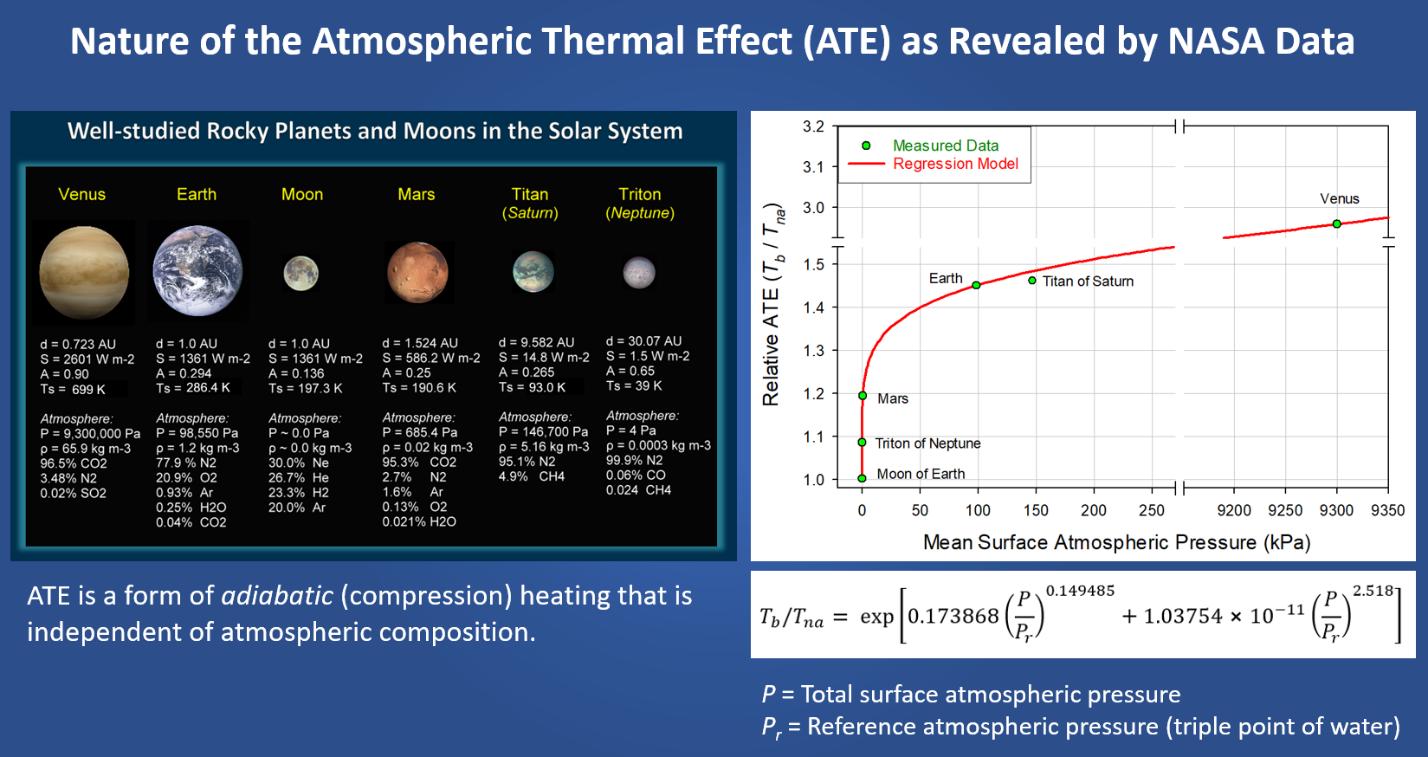
3. Atmospheric longwave radiation is a byproduct (effect) of atmospheric and surface temperatures, which are set by solar heating and pressure. As such, the atmospheric longwave radiation does not impact/affect global surface temperature and climate, since it is simply a cooling mechanism of the atmosphere.

4. The atmospheric “greenhouse effect” has been ill-defined as a difference in the outgoing long-wave flux between Earth’s surface and the top of the atmosphere (TOA) (e.g. Raval & Ramanathan 1989; Schmidt et al. 2010). The observed attenuation of surface longwave fluxes throughout the troposphere, which is in the order of 159 W m-2, has been misinterpreted as an “absorption” (or “trapping”) of radiant heat by greenhouse gases such as water vapor, CO2 and CH4 causing the atmospheric thermal effect. Some scientists call this apparent “absorption” a greenhouse-gas “radiative forcing” (e.g. van Wijngaarden & Happer 2019, 2020, 2023). However, in reality, this flux attenuation is caused by a quasi-adiabatic dissipation (loss) of thermal energy in ascending convective currents due to a decrease of atmospheric pressure with altitude (see Section 4 in Nikolov &Zeller 2024fordetails). Hence,the “greenhouseeffect”andits“radiativeforcing”have de-facto been defined using nonexistent energy. This explains, why the standard definition of the “greenhouse effect” produces nonsensical results (i.e. zero or negative values) over central Antarctica (Schmithüsen et al. 2015; Sejas et al. 2018), where the actual ATE is ~140 K and much larger than the global average ATE of ~90 K (see Nikolov & Zeller 2024 for details).

5. On time scales of thousands to millions of years, the Earth’s climate is driven by changes in total atmospheric mass & surface air pressure, which control the Earth’s baseline temperature. Pressure changes explain the observed polar amplification in the geological records. On time scales of decades to centuries, the climate is modulated by cosmically forced variations of cloud albedo. Albedo changes only cause limited fluctuations of the global temperature around a baseline value set by TSI and total pressure (i.e. about ±1 K) (Nikolov & Zeller 2024).

6. Our research produced a new universal global temperature model that accurately describes the mean average temperatures of rocky planets and moonthroughout the entire Solar System as a function of TSI, total atmospheric pressure and cloud albedo fluctuations. The model is mathematically expressed by the following Equation:

Guest-Editor: Stein Storlie Bergsmark

Klimarealistene

Michelets vei 8 B 1466 Lysaker

Norway

ISSN: 2703-9072

Correspondence:

The Earth’s Variable Rotation: A Climate Regulator

Richard Mackey Independent Scholar

epitrchoidkjx@gmail .com

Vol. 4.3 (2024)

pp.83–91

Abstract

Over the past fifty years geophysicists have established that the planet experiences global warming and cooling episodes that are repeated about every 60 years; that these cycles are driven by decadal variations in the rate of rotation of the Earth; that these variations result from oscillations of the Earth’s inner core; and that these oscillations have their origins in the celestial mechanics of the solar system documented by Laplace in 1799. Laplace showed that the motion of the rotation axis of the Earth is determined fully by both gravitational potentials and kinetic moments. Laplace showed that only the gravitational forces and kinetic moments from other celestial bodies influence the rotation of any one of them.

Throughout the 25-year existence of the Intergovernmental Panel on Climate Change (IPCC), it has refused to mention in any of its many reports the vast body of research published over the last 50 years about the role of the Earth’s variable rotation as a determinant of climate dynamics.

As a result, the IPCC has practiced egregious scientific misconduct (as defined by US and European authorities) since it was established in 1988. The IPCC should be terminated immediately.

Keywords: Earth variable rotation; climate system, global temperature; topological analysis; scientific method; independent and dependent variables; Ockham’s Razor; Isaac Newton; Laplace; atmospheric/oceanic equatorial/inertial waves; scientific misconduct; earthquakes; IPCC.

Submitted 2024-11-30, Accepted 2024-12-01. https://doi.org/10.53234/scc202412/24

1. Introduction

This presentation is about an established relationship between variations in the Earth’s rate of rotation that occurs every six or ten years and global temperature.4 It is, therefore, about one facet of the complex climate system of planet Earth.

The relationship has been established for almost fifty years by observation and reported in the world’s major scientific journals. It does not depend on computer simulations or quantitative models.

There is, no doubt, that the planet’s climate system is exceedingly complex and that the dynamics of the system depend on many factors Cook (2005) Bonan (2024).5

4 The ambiguity about 6 or 10 years is a result of the quality of data used by the scientists. For example, Lambeck and Cazenave (1976) could use only the historical data available at that time, whereas Pfeffer, Cazenave et al (2023) used high quality, precise satellite data.

5 See also the full Bretherton diagram of the Earth System, available here: Next Generation Earth Systems Science at the National Science Foundation | The National Academies Press

2. Scientific Method

The best way to understand climate dynamics as a complex system is the use of the canonical scientific method. The core of the scientific method is the idea that observed variations in phenomena can be explained fully using the concepts of independent and dependent variables in relation to theoretical and analytic systems of understanding. The dependent variable is the phenomena whose variations we seek to explain; the independent variables are those phenomena we consider in order to explain the variations under examination.6

The scientific method guides us to explain observed variations of a dependent variable by means of observed variations of relevant independent variables. The scientific method requires that the two classes of variables are connected by means of theoretical and analytic systems of understanding.7 These systems of understanding are corroborated by evidence that supports the system or refuted (weakened, disproved, contradicted) by evidence that does not support the system.

Sometimes the explanation is timeless; sometimes it is in relation to specified time frames. The scientific method requires that we consider fully all relevant independent variables systematically using the null hypothesis to test the scope for each independent variable to contribute to observed variations in the behaviour of the dependent variable.

At the core of the scientific method is the requirement that hypothesised relationships between dependent and independent variables be verifiable or falsifiable and that those who support competing hypotheses can specify and agree what would constitute corroboration and falsification of their preferred hypothesis. The scientific method says find an explanation and test it thoroughly: science depends on the relentless comparison of hypotheses with reality.

Sir Harold Jeffreys FRS (1891 to 1989) pointed (Jeffreys (1974)) out that the confirmation of a theory is always a statement of a high degree of probability.8 He showed that the probability of a theory has nothing to do with the number of persons who believe in the theory and is not proof in the sense that a mathematical theorem is proved. He explained that a person who states that some hypothesis is universally accepted or proved demonstrates only that they do not understand the scientific method.

The scientific method, which evolved from the ideas of Francis Bacon and Galileo Galileo, amongst others, is based on Sir Isaac Newton’s Rules for the Study of Natural Philosophy

He presented four such rules in his Principia Mathematica, Newton (1687).

The rigorous application Newton’s Rules 1 and 2 is a universal feature of the scientific method.

6 It is customary in all areas of science to make graphs with the independent variable on the horizontal axis and the dependent variable on the vertical axis. In the teaching of science from elementary levels onwards this helps show hypothesised relationships between the cause (the independent variable) and the effect (the dependent variable). In the fields of health and pharmacy, the graphs are called dose-response curves. Those who have done experimental science at secondary or tertiary level would have made similar graphs.

7 The theoretical and analytic systems explain the behaviour of the dependent variable in terms of the independent variable(s). This understanding is best expressed by deriving a dynamical mathematical model from the theoretical and analytic systems of explanatory understanding. Mathematical models without theories lack explanatory authority, but theories without mathematical models are insufficient to advance understanding as they lack adequate predictive capacity.

8 Sir Harold Jeffreys FRS (1891 to 1989) was the leading geophysicist of the early 20th century, and in 1924, published a book that became the bible of geophysics, The Earth: Its Origin, History, and Physical Constitution. He was reader in geophysics at Cambridge (1932–46) and was the Plumian chair of Astronomy and Experimental Philosophy (1945–58). He was the author of two significant books on the scientific method and the theory of probability – Scientific Inference Cambridge University Press (Second Edition) 1957 and the Theory of Probability, Clarendon Press, Oxford (Third Edition) 1961. Harold Jeffreys was knighted in 1953.

As stated by Sir Isaac Newton, these are:9

“Rule 1. No more causes of natural things should be admitted than are both true and sufficient to explain their phenomena.

As the philosopher’s say: Nature does nothing in vain, and more causes are in vain when fewer suffice.10 For nature is simple and does not indulge in the luxury of superfluous causes.

Rule 2. Therefore, the causes assigned to natural effects of the same kind must be, so far as possible, the same.

Examples are the cause of respiration in man and beast, or the falling of stones in Europe and America, or the light of a kitchen fire and the sun, or the reflection of light on our earth and the planets.”

Two highly regarded Newtonian scholars, Dan Densmore and William Donahue, explain the significance of Newton’s rules in this way (Densmore, Dana and Donahue, William, 2003):11

“Newton sees these rules as principles that describe the way we actually think if we are thinking philosophically. Applied to natural philosophy, they are standards of sound reasoning about phenomena, causes, and properties of matter. They describe the working of the mind of a careful thinker – in this application, the working of the mind of a natural philosopher, what we would call scientific thinking.”

3. Canonical Framework for the Climate System

In this canonical framework, the climate system is the dependent variable, and the set of independent variables includes the:

1) Sun’s:

• output of radiation and matter;

• electromagnetic and gravitational fields;

2) epitrochoid motion about the solar system barycentre; and 3) topological structure of the heliosphere.

The dependent variable, the climate system, consists of a number of subsystems, principally the Earth’s:

1. atmospheric systems;

2. ocean systems;

3. coupled atmospheric-oceanic systems;

4. near-surface atmospheric partial pressure

5. near-surface atmospheric density

6. clouds;

7. Rossby and Kelvin waves;

8. rotation;

9 Newton, I., (1687) pages 794-795.

10 Newton is referring to the 14th-century English logician, theologian and Franciscan friar William of Ockham who introduced the principle now known as Ockham’s razor. It is also known as the principle of parsimony or the law of parsimony (Latin: lex parsimoniae). Attributed to William of Ockham, a 14thcentury English philosopher and theologian, it is frequently cited as Entia non sunt multiplicanda praeter necessitatem, which translates as Entities must not be multiplied beyond necessity, although Occam never used these exact words. Popularly, the principle is sometimes paraphrased as The simplest explanation is usually the best one Occam's razor - Wikipedia

11 Densmore, Dana and Donahue, William, (2003) page 303.

9. atmospheric angular momentum; 10. dynamo;

11. electromagnetic field; and 12. global electric circuit.

Some of these subsystems consist of further subsystems, for example: the Earth’s atmosphere contains several major oscillating atmospheric/oceanic systems that have a key role in the regulation of the Earth’s weather and climate. They include the Madden-Julian Oscillation (MJO); the El Niño/Southern Oscillation (ENSO); Quasi-Biennial Oscillation (QBO); the Pacific Decadal Oscillation (PDO); the Interdecadal Pacific Oscillation (IPO); the North Atlantic Oscillation (NAO); the Atlantic Multidecadal Oscillation (AMO); the Indian Ocean Dipole (IOD); and the Arctic Oscillation (AO); and the northern and southern polar vortices, which are two permanent cyclones at the poles.12

4. The Earth’s variable rotation and global temperature

Depending on the variable the variations of which are to be explained, any variable can be either an independent or dependent variable. For example, to examine if the Earth’s rotation contributes to the Earth’s climate dynamics, means considering the Earth’s rotation as an independent variable and the Earth’s climate system as the dependent variable.

If examining the extent to which the Sun, the Moon, and/or the planets of the solar system regulate the rotation of the Earth is the task, the Earth’s rotation would then become the dependent variable; the Sun, Moon and planets would become the independent variables.

Over the last fifty years, geophysicists have established that the 6- or 10-year variation in the Earth’s rotation is a key determinant of climate dynamics. This has been established empirically over this period by more than a dozen scientists who have had their work published in the world’s leading scientific journals.

Furthermore, careful observation has established that there is a time lag of about eight years between changes in the Earth’s rotational speed and surface temperature, and a time lag of about eight years between the electromagnetic event that results in Earth rotation variations and the rotation variations happening.

Overlaying the causative relation between rotation variations and climate dynamics are the processes that originate with the Sun and the Moon (gravitational fields); the Sun (electromagnetic field; output of radiation and matter); the Sun’s epitrochoid motion about the solar system barycentre; the topological structure of the heliosphere; the dynamic processes of the atmospheric/oceanic systems; and the interaction of all processes.

The 6- or 10-year variable rotation arises from the interaction of the above-mentioned processes with the Earth’s inner cores. These processes also give rise to longer cycles, including those of sixty years and one hundred and eighty years.

Sidorenkov (2009) concluded that because long-term variations in the Earth’s rotation can now be determined with great accuracy, the many-year findings he and others have documented show that the long-term variations in the Earth’s rotation present a unique, nature-born integral index of global climate changes.

Lopes et al (2021) showed that there are four causal processes that determine changes to the rate

12 Note that Fagan (1999), (2000) and (2004) has shown how the changes of the climate rendered by these global atmospheric systems have resulted in major historic changes to cultures and societies throughout the world since the dawn of history.

https://scienceofclimatechange.org

and inclination of the Earth’s rotation in accordance with Laplace’s equations:13

§ The planets, particularly the Jovian planets, acting on the Earth/Moon system.

§ The Sun acting on the Earth/Moon system (and on the rest of the solar system).

§ All the planets of the solar system acting on the Sun.

§ The Sun, having been activated by the third process, proceeds to the second process.

Lopes et al (2021) confirmed Laplace’s 1799 analysis that the motion of the rotation axis of the Earth is determined fully by both gravitational potentials and kinetic moments of the solar system. Laplace showed that only the gravitational forces and kinetic moments from other celestial bodies influence the rotation of any one of them.

Throughout the 25-year existence of the Intergovernmental Panel on Climate Change (IPCC), it has refused to mention in any of its many reports the vast body of research published over the last 50 years about the role of the Earth’s variable rotation as a determinant of climate dynamics. Not representing in the research record accurately by the deliberate omission of scientific results, constitutes the falsification of science and is scientific misconduct.14

The IPCC may well continue its characteristic unscientific egregious obduracy in respect of the topological analysis applied to the behaviour of atmospheric/oceanic equatorial/inertial waves. However, if the IPCC attempts to incorporate the elegant theories and findings of topological analysis, it will have to accept the central role of the Earth’s variable rotation in climate dynamics. Once that is accepted, the IPCC will find that there is no role for Carbon Dioxide that is additional to already well-known determinants of climate dynamics.

The IPCC has, therefore, practiced egregious scientific misconduct since it was established. Accordingly, the IPCC should be terminated immediately.

The unscientific way in which the IPCC deals with those who show the IPCC flaws, parallels the unscientific way in which, between the 1920s and 1967, established geologists tried to stifle the theory of continental drift.

However, the adverse impact of the IPCC’s chimerical theory in comparison to the adverse impact of the false theory of fixed continents, is considerably worse. The IPCC has succeeded in inflicting economic and financial hardship on most of the world and creating the secular religion of Climatism.

The theory of continental drift triumphed because of the careful and thorough scientific work of physicists and mathematicians outside of the discipline of Geology. A similar development is now happening in Climate Science as a result of recently published, high quality scientific work by physicists and mathematicians. They have applied topological analysis to the atmospheric/oceanic equatorial/inertial waves that drive massive systems such as the El Nino Southern Oscillation (ENSO) and the Madden-Julian Oscillation (MJO). These major global atmospheric/oceanic systems drive climate dynamics in significant ways.

ENSO is the primary driver of global climate and the associated patterns of precipitation, productivity and forest mortality. There is a strong relationship between ENSO and seasonal rainfall variability in eastern Australia. The impact of ENSO on Australian rainfall has been known for

13 https://en.wikipedia.org/wiki/Pierre-Simon_Laplace

14 According to the U.S. Office of Science and Technology Policy (National Academy of Sciences), the US National Academy of Engineering and the US Institute of Medicine Committee on Science, Engineering, and Public Policy (National Academy of Sciences (2009)), and endorsed by the Organisation for Economic Co-operation and Development (OECD Secretariat (2022)).

https://scienceofclimatechange.org

decades. ENSO is an important climate phenomenon, especially influencing tropical and subtropical regions, with significant impact on much of Australia’s climate. The MJO is a major source of intraseasonal rainfall variability, especially in the tropical Indo-Pacific region. Its impact has long been known to extend into northern Australia during summer.

5. Ockham Rules

The elegant simplicity that results from the application of Sir Isaac Newton’s Rules, means that there should be one theory of climate dynamics for the solar system; or more precisely, one theory of climate dynamics for any solar system!

Funding: Nil.

Guest-Editor: Stein Storlie Bergsmark

Acknowledgements: I wish to thank professor Emeritus Jan-Erik Solheim for his encouragement.

References

Anderson, D L (1974) Earthquakes and the rotation of the Earth. Science Vol 186, Issue 4158, pp 49 to 50; 4 October 1974.

Bendick, Roger and Bilham, Rebecca (2017) Do weak global stresses synchronize earthquakes? Geophysics Research Letters, 44, 8320–8327.

Bonan, G. B., et al (2024) Reimagining Earth in the Earth system; Journal of Advances in Modeling Earth Systems, 16, e2023MS004017. https://doi.org/10.1029/2023MS00401

Bostrom, R.C. (2000) Tectonic Consequences of the Earth's Rotation United Kingdom: Oxford Univ Press.

Cook, Kerry H (2005) Climate Dynamics, 2nd Edition Princeton University Press.

Courtillot, V, Le Mouel, J L, (1976) On the long-period variations of the Earth's magnetic field from 2 months to 20 years J of Geophysical Research Vol 81 No17 pp 2941–2950 doi:10.1029/JB081i017p02941 (10/06/ 1976).

Courtillot, V et al (2023) On variations of global mean surface temperature: When Laplace meets Milankovic; arXiv preprint arXiv:2306.03442, June 2023.

Currie, R. G., 1973 The - 60 year spectral line in length of day fluctuations, South African Journal of Science, 69, 180-182.

Currie, Robert G, (1980) Detection of the 11-yr sunspot cycle signal in Earth rotation, Geophysical Journal International, Volume 61, Issue 1, April 1980, Pages 131–140.

Delplace, Pierre, Marston, J B, and Venaille, Antoine 2017 Topological Origin of Equatorial Waves; Science Nov 24, 2017; Vol 358 Issue 6366:1075-1077. doi: 10.1126/science.aan8819, Epub 2017 Oct 5. PMID: 28982798.

Densmore, Dana and Donahue, William, 2003. Newton’s Principia: The Central Argument. Third Edition Green Lion Press Santa Fe, New Mexio.

Dickey, Jean O, Marcus, Steven L & De Viro, Olivier (2011) Air Temperature and Anthropogenic Forcing: Insights from the Solid Earth Notes and Correspondence Journal of Climate Vol 24, 15 January 2011.

Duhau S and de Jager C (2012) On the Origin of the Bi-Decadal and the Semi-Secular Oscillations in the Length of the Day, in S. Kenyon et al. (eds), Geodesy for Planet Earth, International Association of Geodesy Symposia 136, Springer -Verlag Berlin Heidelberg, pp. 507-551.

Science of Climate Change

https://scienceofclimatechange.org

Duhau S and Martinez EA (1995) On the Origin of the Length of the Day and the Geomagnetic Field on the Decadal Time Scale, Geophysical Research Letters Vol 22, pps 3283-3288.

Fagan, B., 1999. Floods, Famines and Emperors. El Nino and the Fate of Civilizations Basic Books.

Fagan, B., 2000. The Little Ice Age. How Climate Made History 1300-1800. Basic Books.

Fagan, B., 2004. The Long Summer. How Climate Changed Civilization. Basic Books.

Heck, Bernard, Rummel, Reinhard, Groten, Erwin and Hornik, Helmut (1999) National Report of the Federal Republic of Germany about geodetic activities in the years 1995 to 1999. A Report to the XXII General Assembly of the International Union for Geodesy and Geophysics (IUGG) 1999 in Birmingham; Verlag der Bayerischen Akademie der Wissenschaften in Commission at C. H. Beck'schen Verlagsbuchhandlung Munich 1999.

Jeffreys, H (1974) Theoretical aspects of continental drift. In: Kahle, C.F. (ed.) Plate TectonicsAssessments and Reassessments. The American Association of Petroleum Geologists, Memoir 23, 395–405.

Jochmann, H and Greiner-Mai, H (1996) Climate variations and the Earth’s rotation Journal of Geodynamics Vol 21, No. 2, pp 161-176 1996.

Jochmann, H and Greiner-Mai, H (1997) Correction to ‘Climate variations and the Earth’s rotation’ Journal of Geodynamics Vol 25, No 1, p 14.

Kim, Ji-Eun and Zhang, Chidong, 2021 Core Dynamics of the MJO; Journal of the Atmospheric Sciences Vol 78, 01 January 2021 pps 229–248 doi: https://doi.org/10.1175/JAS-D-20-0193.1

Kirov, B.; Georgieva, K.; Javaraiah, J., (2002) 22-year periodicity in solar rotation, solar wind parameters and Earth rotation. In Solar variability: from core to outer frontiers. The 10th European Solar Physics Meeting, 9 - 14 September 2002, Prague, Czech Republic. Ed. A. Wilson. ESA SP-506, Vol. 1. Noordwijk: ESA Publications Division, ISBN 92-9092-816-6, 2002, p. 149 to 152.

Lamb, H. H. (1972) Climate, present, past and future, Volume 1 Methuen and Co., London. (Note: Volume 2 was published in 1977).

Lambeck, K (1980) The Earth’s Variable Rotation-Geophysical causes and consequences, Cambridge University Press.

Lambeck, K and Cazenave, A (1976), Long Term Variations in the Length of Day and Climatic Change Geophysical Journal of the Royal Astronomical Society Vol 26 Issue No 3 pps 555 to 573.

Liu Shi-Kuo, Liu Shi-Da, Fu Zun-Tao, 2000 Earth rotation and El Nino – Theory of waves; Chinese Journal of Geophysics Vol 43, No 2, pp 167 to 174; https://doi.org/10.1002/cjg223

Lopes, F, Le Mouel, J L, Courtillot, V and Gilbert, D (2021) On the shoulders of Laplace Physics of the Earth and Planetary Interiors Vol 316, July 2021.

Mackey, R., (2007). Rhodes Fairbridge and the idea that the solar system regulates the Earth’s climate. Journal of Coastal Research, Special Issue 50 (Proceedings of the 9th International Coastal Symposium), 955 – 968. Gold Coast, Australia. (PDF) Rhodes Fairbridge and the idea that the solar system regulates the Earth's climate (researchgate.net).

Mackey, R, 2023a Lessons from the Continental Drift controversy for the IPCC debacle; Science of Climate Change Volume 3.5 pp. 487-520 https://doi.org/10.53234/scc202310/24

Mackey, R 2023b The Earth’s decadal rotation and climate dynamics; Science of Climate Change Vol. 3.2 (2023) pp. 119-172, https://doi.org/10.53234/SCC202304/06.

Marcus, Steven L (2016) Does an Intrinsic Source Generate a Shared Low-Frequency Signature

Science of Climate Change

https://scienceofclimatechange.org

in Earth’s Climate and Rotation Rate? Earth Interactions Vol 20 Paper No. 4, 14 pages (Earth Interactions is a joint publication of the American Meteorological Society, American Geophysical Union, and American Association of Geographers).

Mazzarella, Adriano, (2007) The 60-year solar modulation of global air temperature: The Earth's rotation and atmospheric circulation connection, Theoretical and Applied Climatology Vol 88, No. 3) pp 193-1999.

Mazzarella, A and Palumbo, A (1988) Earth’s rotation and solar activity Geophysical Journal 97, 169-171.

Morner, N.A. (1995) Earth rotation, ocean circulation and paleoclimate; GeoJournal 37, 419–430.

Morner, N.-A. (2010) Solar Minima, Earth’s rotation and Little Ice Ages in the 1020 past and in the future The North Atlantic-European case, Global Planet. Change, 72, 282-293, doi:10.1016/j.gloplacha.2010.01.004.

National Academy of Sciences (2009): National Academy of Sciences, National Academy of Engineering (US) and Institute of Medicine (US) Committee on Science, Engineering, and Public Policy. On Being a Scientist: A Guide to Responsible Conduct in Research: Third Edition. Washington (DC): National Academies Press (US); 2009. From: https://www.ncbi.nlm.nih.gov/books/NBK214564. See also Federal Policy on Research Misconduct Office of Science and Technology Policy ORI - The Office of Research Integrity (hhs.gov). OECD Secretariat (2022) Integrity and Security in the Global Research Ecosystem; OECD Science, Technology and Industry Policy Papers June 2022 No. 130; Authorised by the OECD Committee on Scientific and Technological Policy on 15/05/2022.

Newton, I., (1687) Mathematical Principles of Natural Philosophy. A New Translation by I Bernard Cohen and Anne Whitman assisted by Julia Budenz. Preceded by A Guide to Newton’s Principia by I. Bernard Cohen University of California Press USA 1999.

Palumbo, J R (1986) Lunar and solar tidal components in the occurrence of earthquakes in Italy; Geophysical Journal International, Vol 84, Issue 1, January 1986, pp 93–99.

Pfeffer, Julia, Anny Cazenave, Séverine Rosat, Lorena Moreira, Mioara Mandea, Véronique Dehant, Benjamin Coupry, (2023) A 6-yearcycle in the Earth system, Global and Planetary Change, Vol 229, 104245, ISSN 0921-8181, https://doi.org/10.1016/j.gloplacha.2023.104245 (https://www.sciencedirect.com/science/article/pii/S0921818123002187

Rozelot, J P and Spaute, D (1990) Earth Rotation and Climatic Periodicities in McCarthy, Dennis D and Carter, William E (eds) (1990) Variations in Earth Rotation, Geophysical Monograph Series Volume 59 1 January 1990 the American Geophysical Union.

Scafetta, N and Bianchini, A (2023) Overview of the Spectral Coherence between Planetary Resonances and Solar and Climate Oscillations; Climate 2023, Vol 11, Issue 4; 34 pages.

Sidorenkov, N. (2009) The Interaction Between Earth’s Rotation and Geophysical Processes Wiley VCH.

Stoyko A, Stoyko N (1969) Rotation de la terre, phenomenes geophysiques et activite du soleil. Bulletin Academic Royal Belgique 5: 279-285. (Rotation de la terre, phénomènes géophysiques et activité du soleil - Persée (persee.fr)).

Tolstikov, A S, Tissen, Viktor M and Simonova, Galina V (2019) Long-term climate prediction by means of Earth rotation rate adaptive variations models, Proc. SPIE 11208, 25th International Symposium on Atmospheric and Ocean Optics: Atmospheric Physics, 1120887 (18 December 2019).

Venaille, Antoine and Delplace, Pierre, (2021) Wave Topology Brought to the Coast, Physics Review Research Vol 3, 043002, doi.org/10.1103/PhysRevResearch.3.043002.

Science of Climate Change

https://scienceofclimatechange.org

Wilson I R G (2013) Are Changes in the Earth's Rotation Rate External Driven and Do They Affect Climate? The General Science Journal, 3812, pp 1-31.

Yang, Y. and X.D. Song, (2023) Multidecadal variation of the Earth’s inner core rotation, Nature Geoscience, 23 Jan 2023.

Xu, W, Fox-Kemper, B, Lee, Juing-Eun, Marston, Brad, and Zhu, Ziyan (2024) Topological Signature of Stratospheric Poincare´ -Gravity Waves; Journal of the Atmospheric Sciences Vol 81, May 2024; pp 923 to 931

Zheng, DW and Zhou, YH (1995) Research on the relationship between Earth’s variable rotation and global seismic activity. Acta Seismologica Sinica 8, 31–37.

Zotov L, et al., (2016) A possible interrelation between Earth rotation and climatic variability at decadal time-scale, Geodesy and Geodynamics, Vol 7, No 3 pp 216 to 222

Zotov, Leonid, Bizouard, Christian, Sidorenkov, Nikolay, Ustinov, Artem, Ershova, Tatiana (2020) Multidecadal and 6-year variations of LoD Journal of Physics Conference Series Vol 1705 Fundamental and applied problems of mechanics (FAPM) 9-12 January 2020, Moscow, Russian Federation. Published under licence by IOP Publishing Ltd.

https://scienceofclimatechange.org

Klimarealistene

Michelets vei 8 B 1366 Lysaker

Norway

ISSN: 2703-9072

Correspondence:

milo_sir@yahoo.com

Vol. 4.3 (2024)

pp.92–99

The 60-year Cycle of Earth's Climate and the Eccentricity of Jupiter's Orbit

Pavel Kalenda1, Miloslav Šír2, Miroslav Tesař2

1CoalExp, Pražmo, Czech Republic

2Czech Water Management Society, České Budějovice, Czech Republic

Abstract

The 60-year cycle of eccentricity of Jupiter's orbit is shown to be closely related to the 60-year cycle of Earth's climate. Changes in Jupiter's orbit affect the Earth's rotation rate. The following phenomena have been shown to be related to these changes: the 1992 El Chicon eruption, the 1991 Pinatubo eruption, the occurrence of strong earthquakes in the period 1900–2022, the AMO index, low flows in the period 1920–2020 on the Punkva River in the Moravian Karst, precipitation extremes in the Czech Republic after 1995, the catastrophic floods of 2002 in Central Europe, and the unusually long drought of 2014–2019 in Central Europe.

Keywords: Climate cycles; Earth's rotation rate; Jupiter’s orbital eccentricity

Submitted 2024-11-27, Accepted 2024-11-27. https://doi.org/10.53234/scc202412/25

1. Introduction

Many papers analysing climate change periods show (e.g., Schlesinger, Ramankutty 1994; Scafetta 2012, 2019) that a period of about 60 years is very significant in several climate parameters (AMO, PDO, global temperature, sea level, Palmer drought index, etc.), but also in a number of geophysical parameters (LOD, seismicity, volcanic activity). We therefore looked for the cause of this cyclical effect on the Earth.

2. Cyclical influences on climate and geophysical parameters

We have identified three physical mechanisms that cyclically influence climate and geophysical parameters. (Kalenda, Šír 2021; Šír et al. 2022):

(1) The gravitational influence of the planets in Solar System planets on solar activity (Mackey 2007).

(2) The transfer of the orbital rotational moments of all Solar System bodies to the spin rotational moment of the Earth, which affects the motion of the atmosphere, the ocean, and the solid Earth (Kalenda, Malek 2008). Jupiter, together with the Sun, plays a dominant role and has the greatest influence on the rotational momentum of the solar system bodies. The physical mechanism of the transfer of rotational moments from one body to another is described, for example, by Wilson et al. (2008) and Wilson (2013).

(3) The tidal action of Solar System bodies on atmosphere, ocean and solid Earth.

The gravitational influence of the planets of the Solar System on the activity of the Sun has the following periods:

(1) A dominant 11-year (22-year) period, generated mainly by the tidal action of the planets

https://scienceofclimatechange.org

(Mercur-Venus-Earth-Jupiter) on the Sun.

(2) The nearly 60-year impact period of Jupiter-Saturn relative to Uran-Neptun, which distinguishes a 60-year period of ordered and 120-year period of chaotic motion of the Sun around the barycenter of the Solar System in the José cycle of 178.9 years (Charvátová 1988 ; Mackey 2007).

(3) The 60–62-year long period of Jupiter's eccentricity.

(4) Common periods of all planets in the Solar System, including Plane Nine (Batygin, Brown 2021), which give rise to climatic periods of 89 years (Gleisberg period) and 6256.5 years (Xapos-Burke cycle).

The approximately 60-year period of solar activity is evident, for example, in all temperature series and subsequently in the series of global ocean level heights (Jevrejeva 2008). It is also manifested in auroras (Křivský, Pejml 1988; Scafetta 2012), which have nothing to do with the Earth's climate.

Figure 1: AMO index (blue) and the Jupiter's orbital eccentricity (red) during the period 1856–2023.

Source: AMO [online], Jupiter's orbital eccentricity (Bretagnon, Francou 1988)

The transfer of Jupiter's orbital rotational momentum to the Earth's spin rotational momentum is influenced by the eccentricity of Jupiter's orbit (Bretagnon, Francou 1988). The latter is subject to changes that have two fundamental periods of about 900 years and 61 years:

(a) The approximately 900-year period is closely related to three warm climatic periods in the last 2000 years: the Roman climatic optimum of 250–400, the Medieval climatic optimum of 950–1250, and the current warm period after 1980. During the two historical warm periods, the greatest reduction in Jupiter's orbital eccentricity occurred while solar activity was high (Steinhilber 2009). In the current warm period, solar activity and Earth's climate have a similar pattern to the two previous warm periods.

(b) The 61-year period is represented by the climate index AMO (Atlantic Multidecadal Oscillation), which is defined by the water temperature in the North Atlantic (0°–70°N). Fig. 1 shows the AMO index and the Jupiter's orbital eccentricity during the period 1856–2023. It clearly shows that the evolution of the AMO index from 1980 to the present is no different from the previous evolution during the period 1856–1980. The course of the AMO index correlates well (even in phase) with the course of the evolution of the eccentricity of Jupiter's orbit, because the transfer of Jupiter's orbital momentum to the Earth's spin rotational momentum affects the motion of the atmosphere and ocean, and hence the temperature of the water in the North Atlantic. Consequently, the approximately 61-year cycle is very evident in the changes in the positions of pressure bodies in the atmosphere and the associated synoptic frequencies,

Science of Climate Change

https://scienceofclimatechange.org

Jupiter's orbital eccentricity

precipitation intensities and river flow magnitudes in central Europe (Kalenda, Šír 2021; Kalenda et al. 2021; Šír et al. 2022).

3. Earth's rotation rate LOD as a key parameter

The influence of Jupiter on the spin rotation moment of the Earth is reflected in the deviation of ΔLOD from the Earth’s standard rotation period 86,400 seconds (Length of Day). Fig. 2 shows that ΔLOD has a similar pattern to the eccentricity of Jupiter's orbit. The deviations of both quantities are caused by the gravitational effects of other bodies outside Jupiter, particularly the effect of Saturn. Many papers suggest that the Earth's rotation rate LOD is a key parameter that determines both climate and climate-independent geophysical parameter changes.

Figure 10: Jupiter's orbital eccentricity during the period 1856–2023 with a period of 60–63 years (red) and the deviation of ΔLOD from the Earth’s standard rotation period 86,400 seconds with periods of 60–63 years and of about 10 years (blue). Source: IERS [online], Jupiter's orbital eccentricity (Bretagnon, Francou 1988)

Figure 11: Differential Benioff's graph for M8+ events expressing the difference from the mean released seismic moment (blue), Jupiter's orbital eccentricity shifted by +18 years (red). Source: USGS [online], Jupiter's orbital eccentricity (Bretagnon, Francou 1988)

In the Fig. 2, large changes in LOD in about 60-year cycle and small changes in about 10-year cycle are clearly visible. Changes in LOD cause variations in the Coriolis force, which affects the rotation of the solid Earth, atmosphere and ocean currents. This is well observed in the frequency of earthquakes (Fig. 3) and volcanic eruptions. Changes in LOD result in weather and climate fluctuations, as shown at the scale of the Czech Republic by the course of the synoptic situations (Kalenda, Šír 2021), droughts (Fig. 4), floods (Fig. 5, Fig. 6), and on the scale of the whole Earth

Science of Climate Change

https://scienceofclimatechange.org

by AMO index (Fig. 1) and variations in global temperature (Schlesinger, Ramankutty 1994, Dickey et al. 2011, Mackey 2023).

There are two well-known cycles in the LOD and periodical global temperature changes (Mackey 2023):

1) 10-year cycle: Roughly every ten years, the Earth's rotation rate increases or decreases significantly by three to five milliseconds (Fig. 2). These decadal rotational variations likely arise from gravitationally driven electromagnetic coupling between inner and outer cores and the mantle. When the Earth's rotation rate increases over a ten-year period, the Earth is warming globally; when the rate decreases, the Earth is cooling globally. Global temperature changes some eight years after the Earth’s rotation rate changes (Dickey et al. 2011). The most recent estimates of temperature changes accompanied by 10-year changes in the Earth's rotation rate are ± 0.8 ºC.

2) 60-year cycle: Cycles of global warming and cooling repeat approximately every 60 years. These 60-year cycles may be due to changes in the Earth's rotation rate caused by changes of Jupiter's orbital angular momentum, which is expressed by changes of its orbital eccentricity (Kalenda, Šír 2020).

Figure 12: Observed extremely low flows of the Punkva River in the Moravian Karst in Czech Republic (red bars) and the eccentricity of Jupiter's orbit (blue). Source: Lejska et al. (2019), Jupiter's orbital eccentricity (Bretagnon, Francou 1988)

4. The influence of the LOD on weather at the small catchment scale

At the small catchment scale, the rate of the earth's rotation significantly affects precipitation and runoff, as shown in the Liz catchment example (Fig. 5, Fig. 6). The Liz basin lies in the foothills of the Šumava Mts. (Bohemian Forest). The closing profile is located at 49.0697603N, 13.6820850E. The Liz catchment area is situated on a slope between 828 and 1024 m above sea level with a mean slope of 16,6 %, the catchment area is 0.998 km2. The geological subsoil is made up of paragneiss, the soil cover is made up of dystric Cambisol. The catchment area is covered with mature spruce forest.

Fig. 5 shows that the 1982 El Chicon eruption was preceded by a significant decrease and reincrease in eccentricity in the period between 1979 and 1982 with a minimum in 1981. The 2002 catastrophic floods in the Czech Republic, Italy, Spain, Austria, Germany, Slovakia, Hungary, Romania, Bulgaria, Croatia, Ukraine and Russia were preceded by a sharp increase in eccentricity from 1998. Both episodes of significant changes in the eccentricity of Jupiter's orbit are indicated by ovals in Fig. 5.

Figure 13: Catastrophic flood in 2002 in the Czech Republic demonstrated on the Liz basin in the Bohemian Forest. Ovals indicate significant changes in Jupiter’s orbit eccentricity (the red line). The blue (green) bar – precipitation (runoff) depths for the hydrological year November 1 – October 30, the black line – the length of the interannual transition, the empty arrows – the year of the 1982 El Chicon and 1991 Pinatubo eruptions and the 2002 flood. Source: IH [online], VSOP87 [online]

Figure 6: Interannual precipitation-runoff transitions in the Liz basin and deviation of ΔLOD (milliseconds) from the standard rotation period of 86400 seconds (the red line) for the hydro-logical years 1976–2018. The blue (green) bar – precipitation (runoff) depths for the hydrological year November 1 – October 30, the black line – the length of the interannual transition, empty arrows – the year of 1982 El Chicon eruption and 1991 Pinatubo eruption, and 2002 flood, the orange arrow – acceleration of Earth's rotation, the brown arrow – the deceleration of the Earth’s rotation, the black arrow – the increase in standard deviation of transition length after 1995. Data source: IH [online], IERS [online]

In Fig. 6, the black arrow marks the onset of climate extremalisation after 1995. This is characterised by an increase in the inter-annual differences in rainfall and runoff. The strong 1991 Pinatubo eruption (VEI 5) resulted in a planet-wide decrease in atmospheric clarity until 1996 (Keen 2019). After the atmosphere cleared in 1996, however, large interannual differences in precipitation continued. Therefore, volcanic pollution of the Earth's atmosphere in 1991 cannot be considered the cause of the ongoing climate change. The cause was probably the acceleration of the Earth's rotation rate in 1995.

5. Conclusions

We present a causal chain that links a 60-year period of Jupiter's orbital eccentricity to a 60-year period of climate change:

1) 60-year cyclic changes in the eccentricity of Jupiter's orbit are the main cause of changes in the Earth's orbital rate.

2) Changes in the Earth's orbital rate cause climate changes with a period of about 60 years.

A close relationship to changes in the Earth's orbital rate has been demonstrated in the following phenomena:

1) 1992 El Chicon eruption, 2) 1991 Pinatubo eruption, 3) occurrence of strong earthquakes in the period 1900–2022, 4) AMO index,

5) low flows in the period 1920–2020 on the Punkva river in the Moravian Karst, 6) post-1995 rain extremes in the Czech Republic, 7) catastrophic floods 2002 in the Central Europe, 8) unusually long drought 2014–2019 in the Central Europe.

The accumulation of extreme events (6 to 8) in a short period is seen by some climatologists as evidence that essentially irreversible climate change is already underway. In contrast, we believe that this is a periodic climate change caused by the gravitational interaction of solar system bodies on the Earth and the Sun.

Guest-Editor: Stein Storlie Bergsmark

Data

AMO [online]: Atlantic Multidecadal Oscillation Index. https://www1.ncdc.noaa.gov/pub/data/cmb/ersst/v5/index/ersst.v5.amo.dat

IERS [online]: Earth orientation parameter.

https://www.iers.org/IERS/EN/Science/EarthRotation/UT1LOD.html https://datacenter.iers.org/data/latestVersion/224_EOP_C04_14.62-NOW.IAU2000A224.txt

IH [online]: Institute of Hydrodynamics. https://www.ih.cas.cz/en/ USGS [online]: Earthquake Hazards Program. https://www.usgs.gov/programs/earthquake-hazards/earthquakes

References

Bretagnon, P., Francou, G., 1988: Planetary Theories in rectangular and spherical variables: VSOP87 solution, Astronomy and Astrophysics, 202, 309–315 https://api.semanticscholar.org/CorpusID:118273488

https://scienceofclimatechange.org

Brown, M. E.; Batygin, K., 2021: The Orbit of Planet Nine, The Astronomical Journal, 162 (5): 219. arXiv:2108.09868 https://doi.org/10.3847/1538-3881/ac2056

Dickey, J. O., Marcus, S. L., Viron, O., 2011: Air Temperature and Anthropogenic Forcing: Insights from the Solid Earth, Journal of Climate, 24(2), 569–574 https://doi.org/10.1175/2010JCLI3500.1

Charvátová, I., 1988: The solar motion and the variability of solar activity, Adv Space Res, 8, 7, 147–150 https://doi.org/10.1016/0273-1177(88)90184-6

Jevrejeva, S., Moore, J. C., Grinsted, A., Woodworth, P. L., 2008: Recent global sea level acceleration started over 200 years ago? Geophys Res Lett, 35, L08715 https://doi.org/10.1029/2008gl033611

Kalenda, P., Málek, J., 2008: Is solar activity connected with the variations of momentum of Sun? (In Czech: Je sluneční aktivita spojená s variacemi momentu hybnosti Slunce?), Proc. of the 19th National Solar Physics Meeting, Poprad – Slovakia, pp. 36–44 https://www.researchgate.net/publication/349152235_Je_slunecni_aktivita_spojena_s_variacemi_momentu_hybnosti_Slunce_Is_solar_activity_connected_with_the_variations_of_momentum_of_Sun

Kalenda, P., Šír, M., 2020: Climate cycles caused by variations in solar activity (In Czech: Klimatické cykly způsobené kolísáním sluneční activity), Vodohospodářský Bulletin 2020, 34–38 https://www.researchgate.net/publication/347421603_Klimaticke_cykly_zpusobene_kolisanim_slunecni_aktivity

Kalenda, P., Šír, M., 2021: The influence of Jupiter on the course of typical synoptic situations in the Czech Republic in the period 1946–2019 (In Czech: Vliv Jupitera na chod typických synoptických situací na území ČR v období 1946 – 2019), Vodohospodářský bulletin 2021, 29–34 https://www.researchgate.net/publication/359142983_The_influence_of_Jupiter_on_the_course _of_typical_synoptic_situations_in_the_Czech_Republic_in_the_period_19462019_Vliv_Jupitera_na_chod_typickych_synoptickych_situaci_na_uzemi_CR_v_obdobi_19462019

Kalenda, P., Tesař, M., Šír, M., 2021: Precipitation and river discharge cycles in Central Europe after 1800 (In Czech: Cykly srážek a průtoků ve střední Evropě po roce 1800), Vodohospodářský bulletin 2021, 35–39

https://www.researchgate.net/publication/359143094_Precipitation_and_river_discharge_cycles _in_Central_Europe_after_1800_Cykly_srazek_a_prutoku_ve_stredni_Evrope_po_roce_1800 Keen, R. A., 2019: Two Centuries of Volcanic Aerosols Derived from Lunar Eclipse Records, 1805–2019. In: 47th Global Monitoring Annual Conference 2019, Program and Abstracts Booklet, NOAA Earth System Research Laboratory, Global Monitoring Division https://gml.noaa.gov/publications/annual_meetings/2019/posters/41-Keen.pdf

Křivský, L., Pejml, K., 1988: Solar activity aurorae and climate in Central Europe in the last 1000 years, Publications of the Astronomical Institute of the Czechoslovak Academy of Sciences, No. 75. https://www.asu.cas.cz/~had/PAI75-part1.pdf

Lejska, S., Kuda, F., Kněžínek, K., 2019: A little overview of drought history of the Punkva River, focusing on the year 2018 (In Czech: Malý pohled na historii suchých období v řece Punkvě se zřetelem na rok 2018). In: Bosák, P., Geršl, M., Novotná, J., (eds.) Speleofórum 2019, Praha: Česká speleologická společnost/Czech speleological society, 2019, pp. 16–19 https://invenio.nusl.cz/record/399095?ln=en

Mackey, R., 2007: Rhodes Fairbridge and the idea that the solar system regulates the Earth’s climate, Journal of Coastal Research, Special Issue 50, 955–968 https://doi.org/10.2112/JCR-SI50-176.1

Science of Climate Change

https://scienceofclimatechange.org

Mackey, R., 2023: The Earth’s Decadal Rotation and Climate Dynamics, Science of Climate Change, Vol. 3.2 (2023), 119–172 https://doi.org/10.53234/SCC202304/06

Scafetta, N., 2010: Empirical evidence for a celestial origin of the climate oscillations and its implications, J. of Atmospheric and Solar-Terrestrial Phys., 72 (2010) 951–970 https://doi.org/doi:10.1016/j.jastp.2010.04.015

Scafetta, N., 2012: A Shared Frequency Set between the Historical Mid-Latitude Aurora Records and the Global Surface Temperature, J. of Atmospheric and Solar-Terrestrial Phys., 74, 145–163 https://doi.org/10.1016/j.jastp.2011.10.013

Scafetta, N., 2016: High resolution coherence analysis between planetary and climate oscillations, Adv. in Space Res., 57, 2121–2135 https://doi.org/10.1016/j.asr.2016.02.029

Scafetta, N., Milani, F., Bianchini, A., 2019: Multiscale Analysis of the Instantaneous Eccentricity Oscillations of the Planets of the Solar System from 13 000 BC to 17 000 AD, Astron. Lett., 45, 778–790 https://doi.org/10.1134/s1063773719110094

Schlesinger, M., Ramankutty, E., 1994: An oscillation in the global climate system of period 65–70 years, Nature, 367, 723–726 https://doi.org/10.1038/367723a0

Steinhilber, F., Beer, J. and Fröhlich, C., 2009: Total solar irradiance during the Holocene, Geophys Res Lett, 36, L19704. https://doi.org/10.1029/2009GL040142

Šír, M., Kalenda, P., Tesař, M., 2022: Jupiter climate oscillation 1960–2020 (In Czech: Jupiterská klimatická oscilace v letech 1960–2020), Vodohospodářský Bulletin 2022, 38–42 https://www.researchgate.net/publication/369561316_Jupiter_climate_oscillation_1960_-_2020

Wilson, I. R. G., Carter, B. D., Waite, I. A., 2008: Does a Spin-Orbit Coupling Between the Sun and the Jovian Planets Govern the Solar Cycle? Publ. Astron. Soc. Australia, 25, 85–93 https://doi.org/10.1071/as06018

Wilson, I. R. G., 2013: The Venus-Earth-Jupiter spin-orbit coupling model, Pattern Recogn. Phys., 1, 147–158

https://www.researchgate.net/publication/260670249_The_Venus-Earth-Jupiter_spin-orbit_coupling_model

https://scienceofclimatechange.org

Klimarealistene

Michelets vei 8 B 1366 Lysaker, Norway

ISSN: 2703-9072

Correspondence: pkalenda@seznam.cz

Vol. 4.3 (2024)

pp.100-107

Calculation of Thermal Energy Accumulation from the Behaviour of the Temperature Field in the Near-surface Layers of the Earth’s Crust

Pavel Kalenda1 Ivo Wandrol2 Karel Frydrýšek3

1CoalExp, Czech Republik

2Silesian Unversity in Opava, Czech Republik

3VŠB-TU, Czech Republik

Keywords: Thermal energy accumulation; geomechanics modelling; Earth’s crust

Submitted 2024-11-21, Accepted 2024-11-25. https://doi.org/10.53234/scc202412/26

1. Introduction

We focused on geomechanics/geophysics and modelling the mechanical behaviour of the Earth's crust (lithospheric plates). The main theme was the investigation of exogenous factors in crustal phenomena. Exogenous factors include e.g. tidal forces, cyclic changes in crustal temperature caused by the Sun, repeated changes in atmospheric air pressure, wave energy transfer from water bodies (seas and oceans) into the crust, etc. This paper (extended abstract of presentation) will show conclusions from models that address the effect of surface temperature changes on the behaviour of the Earth's crust. One of the outputs was a calculation of the temperature field over a time interval of two years.

We then created a similar model focusing only on temperature. It is a recursive algorithm to calculate changes in the temperature field in the Earth's crust based on the surface temperature. The results of both models showing the heat penetration into the deep crust are consistent with the measurements. Based on this recursive algorithm, we estimated the amount of thermal energy stored in the Earth's crust. In this way, the time it takes for half of the stored energy to be released back into the atmosphere can be determined. The most likely value for this parameter t1/2 is 270 years, which means that the amount of energy in the entire Earth's crust is now at its maximum. This is due to anomalously high solar activity. The future cumulative solar energy in the Earth's crust is estimated based on estimates of the evolution of solar activity. The results show a small increase in accumulated energy up to 2060 and then a smaller or larger decrease in accumulated energy and hence a decrease in global surface temperature.

2. Model from surface temperature

The most complicated and challenging problem was creating the “surface temperature model” This model will be used as the basis for the future continuation of work on the creation of the above-mentioned geomechanical model. Up to now, the influence of surface temperature changes on stress-deformation states inside the Earth’s crust has been considered insignificant in geophysics. The finite element method (FEM) was used for this purpose; the model was created using MSC.MARC/MENTAT software (planar stress, the Earth’s crust resting on an elastic

https://scienceofclimatechange.org

foundation). The “surface temperature model” is divided into 24 sections. Each section corresponds with one type of material defined via material parameters (the influence of non -homogeneities). Surface temperatures were inserted into the model as limit conditions for a period of two years of real values, measured at meteorological stations. The dissertation also includes statistical calculations for the creation of stochastic models for the process of movement and stress on the surface of the Earth’s crust. The model demonstrated that small temperature changes on the surface and at shallow depths below the surface (up to approx. 30 m) influence the variability of stress at depths of over 10 km [1,2].

An acceptable simplification for the calculations can be achieved by replacing the Earth's crust by an infinite hollow cylinder (see Fig. 1), the so-called ‘Earthcylinder’, and defining the heating or cooling of the Earth's outer surface as a time-varying heat function T=f(φ,t), where φ is the angle /deg/ and t is time /s/ [1].

The Earth's crust is composed of lithospheric plates and is mainly made up of rocks and minerals, where various faults, fractures and other geological formations occur. In addition to rocks and minerals, there are also gases and water. It is, therefore, an inherently highly anisotropic, heterogeneous and inhomogeneous material.

Fig. 1. Model of the Earth as an infinite hollow cylinder, the so-called ‘Earthcylinder’ with heating from the Sun (not to scale)

The model of the Earth's crust is divided into 24 sections with different material properties; it is a piecewise isotropic homogeneous material model, which appears to be anisotropic from the outside. On the surface of each material section, there are temperature functions T# , T! , T!: = f(φ, t), which correspond to time-varying temperature values over a two-year period, see Fig. 2 (overleaf) and [2].

For the FEM calculation, the problem is treated as a planar problem with an assumed plane strain. In Fig. 2, the crustal thickness is highly enlarged (for clarity), and the planar model is shown as being divided into 24 sections, with assigned material properties and loading indicated from the temperature. The angular perimeter is divided by 15 degrees, with a different material in each of the 15 degrees.

2.1 Boundary conditions

The temperature boundary condition T = f(φ, t) (i.e. T# , T! , T!: = f(φ, t), see Figs. 2-4), depends on time t and the angular dimension of the Earth and acts on the outer surface of the crust. This boundary condition simulates the cyclic temperature changes based on the daily cycle of the Earth's rotation and the annual cycle of the planet's orbit around the Sun. An example of T! dependence loading for 2 years and 5 days is shown in Fig. 3.

Fig. 2. ‘Earthcylinder‘ with materials and temperature loads (not to scale)

Fig.3. Temperature T2 distribution (a) Boundary condition – for whole 2 years at node 1

The data were then processed for importing into the MSC. Marc Mentat software [42]. The resulting time-dependent temperature series contained 35424 values. For each subsequent section, the time series is shifted by another hour. The different temperature boundary conditions in each section represent a virtual rotation of the model, i.e. the change in temperature simulates the rotation of the Earth around the Sun.

2.2

Results from FEA

Fig. 4 shows that small temperature changes (selected standard deviation) on the surface (depth h=0 m) and at shallow depths under the surface (up to approx. 30 m – approx. annual penetration)

Proceedings of the International CLINTEL

Fig. 5 shows the depth evolution of the equivalent stress σ;<; at the interface of sections 1 and 2 (i.e. φ = 0°, see Fig. 2). From Fig. 5, the stress attenuation towards depth is evident, as was the case for the other sections. The trend of decreasing σ;<; towards the Earth's interior can also be partly explained by the all-round pressure stress states that characterize matter deep underground or in water.

Fig. 4. Temperature trends in the depth profile at the interface of sections 1 and 2 (φ = 0°) over two years

Fig. 5. Plot of depth evolution of the equivalent van mises stress (HMH)/Pa/ at the interface of sections 1 and 2.

Figs. 5 and 6 show that stress fluctuations of the order of 1 MPa occur at a depth of 10 km, even though the thermal wave reached a depth of only 22 m.

3. Model of heat accumulation in the Earth’s crust

We developed recursive procedure, which allows estimation of the part of solar energy accumulated in the Earth´s crust and estimation of the half-time of the heat radiation/accumulation parameter. This kind of parameter can show time during which one half of the accumulated energy is released back to space. The theoretical relationships were verified by the long-term paedology measurements.

Science of Climate Change

https://scienceofclimatechange.org

Let us have a material cube of infinitesimal small dimensions at the depth h below the surface (half-space), which is thermally bonded with the surrounding material (see F ig. 6).

Fig. 6. Scheme of the penetration of heat from the surface to the depth and its radiation from the cube in the depth h

To derive the relationship, we performed a superposition of Newton's law of body cooling and the Fourier-Kirchhoff heat conduction equation. Then we verified the correctness of the relation on measured data (see Fig.7).

Fig. 7. Comparison of the temperature development in the depth of 2 cm (turquoise) and 100 cm (red) and recalculated temperatures from the depth of 2 cm to the depth of 100 cm (black). Residuals between measured and recalculated temperatures at a depth of 100 cm are blue.

Fig. 7 illustrates the recalculated temperature from the depth of 2 cm to the depth of 100 cm using a recursive relation /16/ and the least squares method for the residues of two parameters ah and bh

Science of Climate Change

https://scienceofclimatechange.org

It can be seen that although the temperature at the depth of 2 cm has a phase shift from the temperature measured at the depth of 100 cm (correlation r = 0.88), after conversion it exhibits a high correlation (r = 0.997) where both curves only shifted by the absolute value of 3.75 ° C, which is probably due to a local geothermal gradient or a paleoclimate development. All recalculated temperatures from the depth of 2 cm to the depths of 10 cm up to 100 cm show a high degree of correlation with the correlation coefficient greater than 0.995 with the measured temperatures at these depths.

For the conversion of energy from the Earth's surface to the depth h, it is necessary to know two parameters: ah and bh. For the analysis of the correlation between the radiated heat from the depth h to the surface and surface temperatures, it is not necessary to know the parameter bh, since it only moves the absolute level of temperature at the depth h compared to the surface of the constant value. Therefore, the correlation coefficient is not dependent on it. We therefore used coefficient bh = 1. On the other hand, the coefficient ah has a real physical meaning and shows how quickly the heat accumulates in the Earth's crust, and/or how quickly it is radiated back to the surface.

3.1 Results of analyses

We calculated for different coefficients ah the correlation coefficient between the two time series: 1) Of the reconstructed surface temperature by Mann et al. (2008) and 2) volume of the heat release from the depth h to the surface (OLR) according to the relationship shown in Fig. 6. Fig. 8 shows the correlation coefficient between the reconstructed global temperature and the heat released from the Earth's crust.

Fig. 8. Correlation coefficient between reconstructed global temperature CRU_composite (Mann et al., 2008) and released heat from the crust for various half-life of heat as a parameter.

It is evident that the correlation coefficient between the smoothed temperatures within the window of 50 years is higher than for the temperature smoothed within a 10-year window, and reaches the maximum r = 0.86, indicating a statistical dependence between the two rows at a significance level of 15 %. The higher correlation coefficient for the longer window shows that the values of the proxy-Wolf numbers in increments of 10 years are physically smoothed, and that the samples did not allow obtaining a higher accuracy either in amplitude or time. Therefore, the smoother curve of the reconstructed temperatures in the 50-year window corresponds better with the primarily smoothed curve of the proxy-Wolf numbers. The resulting curve of heat stored in the continental crust (in relative units) for the maximum correlation coefficient (i.e. the half-time of the heat radiation/accumulation parameter is 270 years) together with the reconstructed temperature

curve, is shown in Fig. 9.

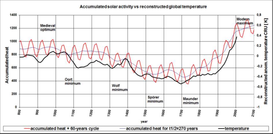
Fig. 9. Comparison between accumulated heat from solar activity and reconstructed global temperature in 50-year time window (according to Mann et al., 2008).

4. Conclusion

The model from surface temperatures showed stress fluctuations on the order of 1 MPa occurring at a depth of 10 km, although the thermal wave reached a depth of only 22 m.

Accumulation of the heat in the Earth´s crust integrates and therefore delays outgoing long wave radiation behind the solar activity. The half-life of the heat coefficient is approx. 270 years.

If we admit that part of the incident energy from the Sun accumulates in the rocks of the continental crust, we can estimate, based on the solar activity and a climatological parameter containing heat or temperature, what the material parameters of these rocks are. The greatest correlation coefficient between the number of the proxy-Wolf numbers [4] and global temperature anomalies in the window of 50 years in the increments of 10 years [5] has been detected for the "half -life of heat" parameter is 270 years. For this parameter, the correlation coefficient between the proxyWolf numbers and reconstructed temperature reached r = 0.86, which is a sign of the fact that there is a link between them.

All of solar cycles are close to their maxima. The sudden drop of solar activity can be supposed. Next, the drop of global temperatures can be expected.

The analysis of the development of the heat stored in the continental crust shows that the currently existing climate changes are caused by nature origin, not mankind [6].

The question is What we understand under „climate changes“. According to our results, it is proportional to the OLR ~ accumulated heat in the Earth´s crust.

Guest-Editor: Stein Storlie Bergsmark

References

[1] Wandrol, I. Modelling of mechanical behavior of the Earth’s crust. 2007. Ph.D. dissertation, Department of Applied Mechanics, Faculty of Mechanical Engineering, VŠB-TU Ostrava, 160 pages, 80 figures, 33 tables, 15 supplements. Tutor: Assoc. Prof., Ing. Karel Frydrýšek, Ph.D, Ostrava, Czech republic, written in Czech language

[2] WANDROL, Ivo, Karel FRYDRYSEK and Daniel CEPICA. Analysis of the Influence of Thermal Loading on the Behaviour of the Earth's Crust. APPLIED SCIENCES-BASEL. 2023, vol. 13, No 7, p. "4367-1"-"4367-24", 24 pp. ISSN 2076-3417. Available from: https://dx.doi.org/10.3390/app13074367

[3] KALENDA, Pavel, Ivo WANDROL, Karel FRYDRÝŠEK and Vítězslav KREMLÍK. Calculation of Solar Energy Accumulated in Continental Rocks. NCGT journal. 2018, vol. 6, No 3, p. 347-360. ISSN 2202-0039.

[4] Solanki, S.K., Usoskin, I.G., Kromer, B., Schüssler, M. and Beer, J. (2004): “Unusual activity of the Sun during recent decades compared to the previous 11,000 years”. Nature, 431, no. 7012, p. 1084–1087. Available from: http://www.cricyt.edu.ar/paleo/pubs/solanki2004/solanki2004.html

[5] Mann, M.E., Zhang, Z., Hughes, M.K., Bradley, R.S., Miller, S.K., Rutherford, S. (2008): Proxy-Based Reconstructions of Hemispheric and Global Surface Temperature Variations over the Past Two Millennia, Proc. Natl. Acad. Sci., 105, 13252-13257.

[6] N.A. Mörner ed. (2015): Planetary influence on the Sun and the Earth and a modern bookburning. Nova Science Publishers, New York. ISBN: 978-1-63482-489-9 (e-Book).

https://scienceofclimatechange.org

Klimarealistene

Michelets vei 8 B 1366

Lysaker Norway

ISSN: 2703-9072

Correspondence

Radiation Data from CERES Measurements – do they agree with Current Climate Dogma?

Milan Šálek

Self employed meteorologist

milan salek@email cz

Vol. 4.3(2024)

pp. 108–110

Keywords: Greenhouse effect; CERES measurements; radiation balance; albedo

Submitted 2024-11-22, Accepted 2024-11-25. https://doi.org/10.53234/scc202412/27

1. Introduction

The term "greenhouse effect" describes a crucial property of certain atmospheric gases that can absorb long-wave radiation and re-radiate it, partially back to Earth's surface. This process keeps the surface temperature approximately 30 °C warmer than it would be otherwise. The primary radiatively active ("greenhouse") gases include water vapor, carbon dioxide, methane, and nitrogen monoxide. However, the actual mechanism differs from that of a physical greenhouse, which also prevents vertical mixing (convection), making the term "greenhouse effect" somewhat misleading.

According to the prevailing climate paradigm (or dogma), the warming observed since 1950 has been predominantly caused by an enhanced greenhouse effect, largely driven by anthropogenic emissions of key greenhouse gases except water vapor, which is mainly considered a feedback agent. This view is endorsed by the Intergovernmental Panel on Climate Change (IPCC), widely regarded as the primary authority on climate change attribution. Notably, these conclusions have been derived mainly from global circulation models.

If this hypothesis holds true, we would expect some decrease in outgoing long-wave radiation at the top of the atmosphere (until we see a noticeable temperature increase), provided other components of the radiation balance remain relatively stable.

Fortunately, the "Clouds and the Earth’s Radiant Energy System (CERES)" project has been measuring Earth’s radiation balance since March 2000, providing us with valuable data. By examining these measurements, we can assess the state of radiation components at the top of the atmosphere.

Surprisingly, the data show a picture quite different from the current climate narrative. Several studies have pointed out that the primary driver of the observed radiation imbalance is rather short-wave reflected radiation, in other words the decreasing planetary albedo. Notable examples include Dübal and Vahrenholt (2021) and more recently Nikolov and Zeller (2024), both of whom suggest that this reduction in planetary albedo is likely the main factor behind the temperature rise in recent decades.

Figure 1 (overleaf) illustrates the global area-weighted averages of the 12-month centered running mean of these radiation components: short-wave outgoing (reflected) radiation, long-wave outgoing radiation, the radiation balance (net flux), alongside the GISTEMP temperature anomaly and incoming solar radiation.

https://scienceofclimatechange.org

GISTEMP temperatures. Twelve-month running means of global quantities.

The data clearly show that the short-wave reflected radiation is the primary contributor to the radiation imbalance. This is particularly apparent over the last 10–15 years. While some changes in the greenhouse effect cannot be ruled out, they are probably not the dominant factor.

The causes of the decreasing planetary albedo are not yet fully understood, though most research points to changes in cloud properties, especially cloud reflectivity, which is influenced by both natural and anthropogenic aerosols. Other potential factors include surface changes, such as urbanization, decrease of ice/snow areas and reforestation.

2. Conclusions

Despite these findings, which have been corroborated by multiple studies, they are largely ignored by mainstream media, including public outlets that should provide balanced information. It is becoming increasingly likely that the intense focus on reducing greenhouse gas emissions may be a misallocation of resources.

This is not to suggest that efforts toward energy conservation or reducing fossil fuel use are totally misguided. However, examining the experiences of countries like France and Germany reveals

that nuclear energy has proven to be the most effective means of decarbonization. Any decarbonization strategy that does not prioritize nuclear energy raises questions about whether the true goal is climate protection or, perhaps, the redistribution of wealth.

Guest-Editor: Stein Storlie Bergsmark

References (not exhaustive)

Dübal, H.-F.; Vahrenholt, F.: Radiative energy flux variation from 2001–2020. Atmosphere 2021, 12, 1297, https://www.mdpi.com/2073-4433/12/10/1297

Nikolov, N.; Zeller, K.F., 2024: Roles of Earth’s Albedo Variations and Top-of-the-Atmosphere Energy Imbalance in Recent Warming: New Insights from Satellite and Surface Observations. Geomatics 2024, 4, 311–341, https://www mdpi com/2673-7418/4/3/17

Wielicki, B. A., B. R. Barkstrom, E. F. Harrison, R. B. Lee III, G. L. Smith, and J. E. Cooper, 1996: Clouds and the Earth’s Radiant Energy System (CERES): An Earth Observing System Experiment, Bull. Amer. Meteor. Soc., 77, 853-868, https://doi org/10 1175/1520-0477(1996)077<0853:CATERE>2 0 CO;2

The script that creates the picture above is freely available at https://github.com/Milan007sys/ceres_graphs/.

Science of Climate Change

https://scienceofclimatechange.org

Klimarealistene

Michelets vei 8 B

1366 Lysaker

Norway

ISSN: 2703-9072

Bond Cycles and the Influence of The Sun on Earth’s Climate

Euan Mearns Energy Matters, Aberdeen, UK

Keywords: Bond cycles; solar influence, Earth’s climate

Correspondence:

uan.mearns@gm ail.com

Vol. 4.3(2024)

Pp 111–114

Submitted 2024-11-25, Accepted 2024-11-29. https://doi.org/10.53234/scc202412/28

Summary of presentation

Bond cycles are named after Gerard Bond, the first author on a seminal paper published in the journal Science in 2001 (from now on simply “Bond”):

Persistent Solar Influence on North Atlantic Climate During the Holocene Gerard Bond, et al. Science 294, 2130 (2001); https://doi.10.1126/science.1065680

At the heart of Bond’s work are two important geological / geochemical processes:

1. Sedimentary provenance analysis is the methodology of linking a sedimentary sequence to its source area. Most sediments and sedimentary rocks have origins in erosion products in uplifted areas of the continental masses. These erosion products are gathered by river systems and transported to the sea where they accumulate on the continental shelves. The main tools employed to determine provenance are:

a. Bulk chemistry

b. Mineralogy, especially exotic minerals

c. Isotope composition

d. Sedimentary structures

2. Cosmogenic isotope variations. Cosmogenic isotopes are formed in the atmosphere by the action of galactic cosmic rays on existing isotopes of N and O most notably to produce 14C and 10Be. Both of these isotopes are naturally radioactive and decay to 14N and 10B respectively.

Bond studied core samples from two deep drilling sites in the N Atlantic. Site MC52 lies to the west of Ireland and site MC21 lies SE of Newfoundland close to the site where the Titanic struck an ice berg and sank (Figure 1). The focus of Bond’s work was the abundance and type of ice rafted debris (IRD) where three types with distinctive provenance were identified, namely a) Icelandic volcanic glass, b) hematite-stained grains (red coloured) from Svalbard and east Greenland and c) detrital carbonate derived from the areas surrounding Baffin Bay and the Labrador Sea (Figure 1). IRD in the N Atlantic is formed when icebergs, that entrained sediment in glaciers or ice shelves, float eastwards or southwards and melt with the result that the IRD drizzles on to the ocean floor. Ice bergs are rare off Newfoundland and are absent west of Ireland today with the implication that in the past, ocean currents and winds periodically had a configuration very different to today with a larger N to S component.

Science of Climate Change

https://scienceofclimatechange.org

Figure 1. Map showing the locations of drilling sites MC21 and MC52 with the complex interpretation of Bond superimposed.

Figure 2 Drift ice index (black solid) displaying Bond Cycles and CO2 concentrations from Taylor Dome (blue) and Law Dome (orange), showing that variance in CO2 has little influence on the drift ice cycles that are believed to be controlled by solar variability. LIA=Little Ice Age, MWP=Medieval Warm Period, DA-Dark Ages, RWP=Roman Warm Period.

Bond summarised the complex provenance – depth profiles for 4 records into a single smoothed and de-trended graph that is reproduced in Figure 2. Ten major cycles representing the waxing and waning of drift ice quantities are recognised (solid black line in Figure 2). These cycles have become known as Bond cycles or Bond events.

Science of Climate Change

https://scienceofclimatechange.org

Bond went on to compare these ice rafted debris cycles with the cosmogenic isotope production rates of 14C and 10Be and found a sufficiently good co-variation to suggest that variations in solar geomagnetic field strength played a key role in modulating N Atlantic Ocean currents and atmosphere circulation (Figure 3).

Figure 3 Comparison of drift ice index (black line) labelled as “marine” with cosmogenic isotopes labelled as “nuclide”, 14C left (blue line) and 10Be right (grey line) extracted from Figure 3 of Bond et al (2001).

Changes in total solar irradiance of the order -0.04% over the last 50 years are both too small and have the wrong sign to explain recent warming. This is used by the climate alarm community to discount the role of the Sun in influencing Earth’s climate. The trouble with this rationale is that accurate measurements of the Sun cover a far too short time span to be meaningful on the millennial time scale. The Sun may have phases of activity that have not yet been accurately observed or measured directly. Ineson et al (2011) report that variations in ultraviolet emissions are much larger than previously assumed. This could be part of a holistic explanation.

Bond’s work is significant for showing that historic climate cycles like The Modern Warm Period, Little Ice Age, Medieval Warm Period, Dark Ages Cold and Roman Warm Periods (Figure 2) are all synchronous with Bond cycles and by inference, these cycles are linked to variations in Solar magnetic field strength. Similar cyclical variation in the length of Alpine glaciers (Joerin et al 2006) also demonstrate these cyclical variations in N Atlantic climate. The sinking of the Viking Grønland Knarr by sea ice off Greenland, circa 1380, also testifies to an increase in sea ice extent as the N Atlantic realm was entering the Little Ice Age. Permafrost in the foundations of Viking houses on Greenland today certainly was not there when the houses were built. Arguably, it is much colder today than it was 1000 years ago when the Vikings settled Greenland.

If we take the mean length of the Bond cycle as 1200 years and the depth of the Little Ice Age as 400 years before 2001 (~1600AD), then we can anticipate another 200 years of warming before the N Atlantic climate once again begins to cool. This is great news for Mankind.

A footnote on calendar dates and years before present

I sometimes find it a little confusing switching between calendar dates (datum birth of Christ) and years before present (years ago). Here I provide a simple ready reckoner. See table overleaf.

Science of Climate Change

https://scienceofclimatechange.org

Period

Roman Warm Period -250 to 400 2274 to 1624

Birth of Christ 0 2024

Medieval Warm Period ~950 to 1250 1074 to 774

Vikings settle Greenland AQer 986 1038

Battle of Hastings 1066 9587

Hvalsey Church built ~1300 724

Little Ice Age ~1300 to 1850 724 to 174

Sinking of Greenland Knarr ~1380 644

Vikings abandon Greenland ~1450 574

Present day 2024 0

References

Gerard Bond, Bernd Kromer, Juerg Beer, Raimund Muscheler, Michael N. Evans, William Showers, Sharon Hoffmann, Rusty Lotti-Bond, Irka Hajdas, Georges Bonani., 2001. Persistent Solar Influence on North Atlantic Climate During the Holocene, Science 294

Sarah Ineson, Adam A. Scaife, Jeff R. Knight, James C. Manners, Nick J. Dunstone, Lesley J. Gray and Joanna D. Haigh., 2011. Solar forcing of winter climate variability in the Northern Hemisphere, Nature Geoscience Letters, https://doi.org/10.1038/NGEO1282

Ulrich E. Joerin, Thomas F. Stocker and Christian Schluchter, 2006. Multicentury glacier fluctuations in the Swiss Alps during the Holocene The Holocene 16

Guest-Editor: Stein Storlie Bergsmark

Science of Climate Change

https://scienceofclimatechange.org

Klimarealistene

Michelets vei 8 B

1366 Lysaker

Norway

ISSN: 2703-9072

Correspondence:

pokorny@enki.cz

Vol. 4.3(2024)

pp. 115–128

Relationships: Sun – Water – Vegetation - Climate

Evapotranspiration and Vegetation’s Role in

Temperature Regulation

Jan Pokornẏ

Vladimír Jirka

Petra Hesslerová

Anna Huryna ENKI, Chech Republic

Keywords: Evotranspiration; vegetation; plants; solar irradiation; radiation balance

Submitted 2024-12-20, Accepted 2024-12-26. https://doi.org/10.53234/scc202412/29

1. Introduction

The principal role of water and vegetation in the distribution of solar energy and in local and global climate is shown on basis of measured data. Poor knowledge of the function of plants in climate formation results in erroneous decision-making in landscape management. The principles of solar energy distribution in the landscape can be understood and verified by measurement at the level of basic physics and biology. Examples are given for measuring the radiation balance of sunny and cloudy days and spring frosts. The role of clouds in solar energy input and heat flux from the surface of the earth to the atmosphere (greenhouse effect) is emphasized. The thermographic images show the essential role of water evaporation (evapotranspiration) in the temperature regime. Vegetation supplied with water has lower surface temperatures than dry surfaces with higher albedo. Based on literature data and our long-term measurements, we have determined an average evapotranspiration value of 100 mg.m-2. s-1 which is equal to latent heat flux 240 W.m2. Drainage, urbanization, deforestation leads to a shift from latent heat of vaporization to sensible heat, and accelerated flow of heated air into the atmosphere. Per 1 km2 this represents a heat flux of 240 MW on a sunny day. The thermodynamic functions of water and vegetation are expressed in terms of ecosystem services. The history of human civilizations shows how deforestation, drainage, and urbanization lead to the drying up of the landscape. It is therefore necessary to recognize the role of plant physiological processes in the conversion of solar energy and the water cycle.

2. Survey of knowledge in schools on plant functions

Research reveals a lack of awareness about how plants influence the atmosphere. We did research in schools involving 600 students and 100 pre–service biology teachers. We asked, “how can plants influence our atmosphere”. We had correct responses on "oxygen production," but there was almost nothing about water. Then, we asked about what part of solar energy is fixed in plant biomass. Only 8 % of people answered correctly, as plants convert less than 5 % of the solar radiation into biomass (actually, less than 1 %).

Next, we asked what happens to the water taken by plant roots and what its fate is. Similar in Europe and other countries: there is almost no awareness of the cooling effect of water evaporation (Ryplová, Pokorný 2020). These findings are consistent with the general phenomenon of plant ignorance, called "plant blindness" in the literature.

https://scienceofclimatechange.org

Fig. 1. Knowledge of students on plant -atmosphere interaction. Didactic survey among 641 Czech students (15 years old) aimed at the understanding of plant – atmosphere Interactions and plant physiological processes.

Fig. 2. Knowledge on water regime of plants

Correct answers (see also Figure 3 overleaf).

• Less than 1 % of solar energy is fixed in plant biomass by photosynthesis. 1100 kWh.m2.year-1 1 kg of plant dry mass.m-2.year-1

• 1 kg dry biomass contains 4 – 5 kWh energy (combustion heat)

• One molecule of CO2 is fixed, one molecule of O2 is released and several hundred molecules of water are evaporated (transpiration)

• On a sunny day: several W.m-2 used by photosynthesis; several hundred W.m-2 used for water evaporation

• Evaporation rate 100 mg.m-2.s-1 = latent/hidden heat flux of 240W.m-2

3. Undergraduate students' knowledge of the impact of plants on the atmosphere

There is an Erasmus project “Education for Plant Literacy15” involving five countries, focused on plant biology. This project aims to incorporate basic facts and information into our educational system on roles of plants in distribution of solar energy and other processes. The project's books will be released till February 2025. These processes can be understood with knowledge of elementary to high school physics and, most importantly, much can be ascertained by measurement.

3. Measurement of solar radiation and radiation balance

SINE SOLE NIHIL SUM…I am nothing without Sun…

• Sun heats Earth of 290 °C (atmosphere would be solid without Sun energy)

• Do we affect distribution of solar energy by landscape management?

• Yes, markedly and we can measure it

• Landscape drying is more serious than increase of global average temperature shows. Can average temperature explain climate extremes (torrential rain, tornadoes, high summer temperature, spring morning frosts)? Gradients drive winds etc.

• Wetlands, forests cool themselves by water evaporation, increase air humidity = fog, clouds and less incoming solar radiation

• We preserve food by drying, freezing (the life processes are stopped), we deprive landscape of water, and it overheats

The sun heats the Earth by 290 °C. Without the sun's energy, the earth's temperature would be close to absolute zero, the atmosphere would be solid.

15 ERASMUS+ project “Education for Plant Literacy” https://planteducation.eu

Science of Climate Change

https://scienceofclimatechange.org

Fig.

Fig. 5 a) Meteorological station and b) Detail of netradiometer with the sensors for measuring shortwave radiation (incident RS↓; reflected Rs↑) and longwave radiation (R1↓; R1↑, Rnl), c) The scheme of incoming solar radiation distribution (Rn = net radiation)

The sun emits shortwave radiation consisting mainly of visible light. Under clear skies, up to 1000 Wm-2 reaches the earth's surface. Part (approx. 20 % in landscape) of the sun's energy is reflected, part is emitted by the earth's surface as longwave radiation, the remaining part is called net radiation. Man's management measures (drainage, deforestation) determine whether the sun's energy is used to evaporate water or to heat the surface, and whether the air is warmed by the warmed surface. Only 1 % of the incident solar energy is stored in plant biomass, by photosynthesis (Pokorný et al. 2010). Photosynthesis of terrestrial plants is associated with water evaporation (transpiration). For every molecule of carbon dioxide taken in and oxygen given out, hundreds of molecules of water evaporate through the leaf stomata.

https://scienceofclimatechange.org

Fig. 4. Spectrum of solar and terrestrial radiation

Let us compare radiation balance measured by net-radiometer on two of the longest days (summer solstice). On a clear day, we have up to 900 W.m-2 of incoming solar radiation, reflection up to 200 W.m-2 and the flux of long-wave radiation into the atmosphere approx. 100 W.m-2. On a cloudy day we get 10 times less solar energy and temperatures of land surface and atmosphere (clouds) are similar (Jirka et al. 2021).

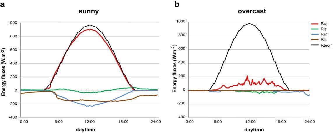
Fig. 6. Daily course of incoming (RS↓), and reflected (Rs↑), solar radiation (W.m-2) and long wave/heat radiation between the sensor and sky (Rl↓), and between the sensor and grass (Rl↑), on the summer solstice 19. 6. 2017 with a clear sky (a) and 21. 6. 2020 with an overcast sky (b). RsTeor↓ shows the theoretical daily course of incoming solar radiation from a clear sky (Jirka et al. 2021).

Fig. 7. Daily course of surface temperature of grass (Trs), air temperature at 2m (Ta2m), temperature of radiometer (Trad), effective temperature of sky (Trsky), temperature of soil at 5cm depth and temperature of dew point (Td) on the summer solstice 19. 6. 2017 with a clear sky (a) and 21. 6. 2020 with an overcast sky (b)

When the absolute humidity of air is low in spring, the sky is cloudless, the solar energy input is strong during the day, the effective temperature of the sky is very low and the flux of longwave radiation into the sky is high. Therefore, the flowers of fruit trees freeze. An example of radiation balance is given below (Pokorný et al. 2023).

https://scienceofclimatechange.org

Fig. 7. Daily course of incoming (RS↓) and reflected (Rs↑) solar radiation (W.m-2) and long wave/heat radiation between the sensor and sky (Rl↓) and between the sensor and grass (Rl↑) on 11- 12 March 2022 (clear sky, low air humidity)

Fig. 8. Daily course of surface temperature of grass (Trs), air temperature at 2m (Ta2m), temperature of radiometer (Trad), effective temperature of sky (Trsky), temperature of soil at 5 cm depth and temperature of dew point (Td) on 11 – 12 March 2022

Table1. Daily sum of incoming solar radiation ∑RS↓ (kWh.day-1.m-2). Daily sum of flow of heat to atmosphere ∑(Rl↓ - Rl↑) (kWh.day-1.m-2). Percentages represent how much energy is radiated from the earth into the sky. 100 % represent incoming solar on a given day. Air humidity and clouds control both incoming solar radiation and flux of heat to sky.

How do we affect clouds? Studies show that the impact of solar radiation is increasing over time from 1980s due to fewer clouds (Wild 2009). Some say it's due to fewer aerosols and cleaner air, but we overlook the effect of vegetation. We forget about evaporation, as mentioned several times, because when we measure long-wave radiation flux from land surface to atmosphere, and it is increasing during the last several decades.

9. Annual average long wave (heat) flux from land surface to atmosphere from 2009 to 2022. Negative values mean increasing long wave radiation (heat) from land to the atmosphere.

4. Thermal imaging and cooling effects

Thermal imaging is illustrative. From the town hall, we observe surface temperatures of the rooftops, which reach 50 °C, surface of parasol 63 °C. In the park, the highest temperature 31 °C have person´s bodies, trees and glass keep temperature under 30 °C. It is not about colour (albedo, reflection), but about evaporation, which is crucial for temperature regulatio n. For an approximate estimate, we can calculate the average value of evaporation 240 W.m-2, equivalent to 100 mg.m2.s-1

Fig.

Fig 10a. Surface temperatures in Třeboň town square on a sunny summer day reach up to 60 °C.

Proceedings of the International

Fig. 10b At the same time surface temperature in the near park do not exceed 30 °C. Trees and grass actively cool themselves by water evaporation, the highest surface temperature have human bodies. They are cooled by the surroundings.

Fig. 11a Surface temperature of a “cultural” landscape on summer sunny day in Třeboň Biosphere Reserve (Czech Republic) at 2 PM, taken by thermographic and visible cameras carried by an Airship

https://scienceofclimatechange.org

Fig. 11b Temperature differences Ts -Ta between surface (Ts) and air temperature (Ta; at 2 m above ground under white screen) at all the studied localities. If the temperature difference is negative (in case of forest, alder stand, wet meadow, water) this is indicative of the cooling ability of the vegetation, which actively cools its surface by evapotranspiration (Hesslerová et al.2013, Pokorný 2019).

With inexpensive instruments we can show the cooling effect of a tree. We look at a tree next to a pavement in full sunshine, where we have 877 W.m-2 incident solar radiation and surface temperature 51 °C. Under the tree, it is 80 W.m-2 and 27 °C. Thanks to the water flux through the tree, which amounts to 20 liters per hour, creating a 14-kilowatt cooling effect. If we replace the tree with an air conditioner, the difference is that air conditioners emit heat, whereas trees direct solar energy to areas high up where water vapor condenses, and latent heat (solar energy) is re-leased. The important thing is the change in volume. One liter of liquid water produces 1,200 liters of water vapor, so when water vapor condenses in clouds, the pressure drops. (Hesslerová et al. 2019, 2021)

Fig. 12 Comparison of surface temperatures on a sunlit pavement and in the shade of a tree. Evaluation of the cooling effect of the tree (Pokorný et al. 2018, Hesslerová et al. 2021).

Dry areas seem innocuous as they don't evaporate water or cause apparent damage. However,

https://scienceofclimatechange.org

they are hot, which causes hot air to rise and draw moisture from nearby ponds and forests. We often hear arguments against creating ponds, wetlands because they "lose" water. Yet, in the forest, there's a temperature inversion cooler below and warmer above. Land drainage, deforestation, land sealing result in shift from evaporation cooling into land surface warming and fast flux of warm air into atmosphere. Decline of evapotranspiration by 240 W.m-2 on 100 ha (1 km2) is linked with release of 240 MW of sensible heat, turbulence and warm ascending air. In our small country we are losing 11 hectares of agriculture land every day. Some other examples from the world give Huryna, Pokorný (2016), Makarieva et al. (2022).

An example of the rise in surface temperatures after forest decline on areas of the order of 100 km2 is shown in Figure 14 a-d. In the Šumava National Park and the Bavarian Forest National Park, mountain forests died after the application of the so-called no-action policy (no management, only natural processes are accepted). On sunny days, surface temperatures rise because water evaporation has decreased. A decrease in evaporation of 240 W.m-2 means an increase in sensible heat of 24 000 MW over an area of 100 km2 (Hesslerová et al. 2017, Hesslerová et al. 2018).

Fig.13a. Definition of the area of interest; source: www.mapy.cz

https://scienceofclimatechange.org

Fig. 13b. Landscape cover of Modrava region according to CORINE LandCover 2006 classification. Yellow = transitional woodland/shrubs after death of mature mountain forest; dark green – coniferous forest, light green – mixed and broad-leaved forest, light brown – fields and meadows, dark brown- peatlands, grey – discontinous urban fabric. Background - Landsat image (27.8.2016), RGB synthesis of channels 564.

Fig. 13c. Surface temperatures on 7th August 1991 (preserved mature living forest), calculated from Landsat thermal channel

https://scienceofclimatechange.org

Fig. 13d Surface temperature calculated from Landsat thermal channel on 27th August 2016. The rise in the surface temperature of the Šumava mountain ridge after the death of the mountain spruce is striking.

5. Conclusions

Lastly, historic civilizations have dried up as deforestation, drainage and urbanization have continued. So, we are faced with a fundamental contradiction: Is evaporation a waste of water, or is it a vital process that sustains life on our planet?

More than 51 % (460 000 km2) of the total area of wetland has been replaced by cropland in the USA since Pre-settlement (Mitsch and Hernandez 2013). Calculating an average shift from latent heat to sensible heat 240 MWkm-2, about 110 000 GW of sensible heat is released during sunny days.

It is a historical experience that deforestation and drying of wetlands leads to a decrease in rainfall and drought. The challenge for science is to explain why this is so and how forests and vegetation in general affect the distribution of solar energy, the water cycle and "why rivers flow". In the last two decades, the field has been growing thanks to satellite research, data availability and biotic pump theory (Makarieva, Gorshkov 2007, Ellison et al. 2017, 2024)

In addition to the numerous negative examples of deforestation, drainage and the subsequent decrease in rainfall and drying, there are increasing attempts to restore the water cycle in the landscape and there are examples of successful solutions. See Kravčík et al (2008), White Paper (2023), Embracing Nature´s Complexity (2024)

A dominant cause of the unsustainability of the world's current market economies is the failure to include the free supporting ecosystem services of the most thermodynamically efficient ecosystems in people's local decision-making about land and landscape. Humanity is thus kept blind to the true thermodynamic values of living landscapes for their own sustenance on Earth. In a short summary article in the peer-reviewed scientific journal Ecosystem Services, we estimated the monetary value of the four basic supporting ecosystem services (cooling and warming, water retention, biodiversity nursery, oxygen production) for essential living landscape cover and found that their monetary values exceed the economic benefits of continued destruction of remnant natural forests and wetlands by up to two orders of magnitude. Therefore, incorporating the monetary values of living nature into human spatial decision-making for restoring thermodynamically functional landscapes is the first and indispensable step towards sustaining the human species on Earth (Seják et al. 2022).

Guest-Editor: Stein

Storlie Bergsmark

References

Ellison, David; Morris, Cindy E.; Locatelli, Bruno; Sheil, Douglas; Cohen, Jane; Murdiyarso, Daniel; Gutierrez, Victoria; Noordwijk, Meine van; Creed, Irena F.; Pokorny, Jan; Gaveau, David; Spracklen, Dominick V.; Tobella, Aida Bargués; Ilstedt, Ulrik; Teuling, Adriaan J. (2017). "Trees, forests and water: Cool insights for a hot world". Global Environmental Change. 43: 51–61.

Ellison, D., Pokorný, J., Wild, M. 2024, Even cooler insights: On the power of forests to (water the Earth and) cool the plane. Glob Change Biol. 2024;30: e17195.

Hesslerová, P., Pokorný, J., Brom, J., & Rejšková-Procházková, A. (2013). Daily dynamics of radiation surface temperature of different land cover types in a temperate cultural landscape: Consequences for the local climate. Ecological Engineering, 54, 145–154.

Hesslerová, P., Pokorný, J., Huryna, H., 2017 Hodnocení vývoje krajinného pokryvu Modravska (NP Šumava) z termálních dat Landsat. Případová studie pro MŽP, 26 stran (In Czech)

Hesslerová, P., Huryna, H., Pokorný, J., Procházka, J., 2018, The effect of forest disturbance on landscape temperature. Ecological Engineering 120, 345 – 354

Hesslerová, P., Pokorný, J., Huryna, H., Harper, D.: 2019, Wetlands and Forests Regulate Climate via Evapotranspiration., In, S. An, J.T.A. Verhoeven (eds.),Wetlands: Ecosystem Services, Restoration and Wise Use, Ecological Studies 238, pp.63 – 93

Hesslerová, P., Pokorný, J., Huryna, H., Seják, J., Jirka, V. (2021). The impacts of greenery on urban climate and the options for use of thermal data in urban areas., Progress in Planning

Huryna, H. and Pokorný, J. 2016 The role of water and vegetation in the distribution of solar energy and local climate: a review. Folia Geobotanica., 51(3), 101-208.

Jirka V., Hesslerová, P., Huryna, H., Pokorný, J., 2021 Energetická výměna mezi zemským povrchem a atmosférou v závislosti na meteorologických podmínkách bez ohledu na obsah CO2. Vytápění, větrání, instalace. 5/ 2021, str. 234 - 239

Kravčík, M. Pokorný, J., Kohutiar, J.,Kováč, M., Tóth, E. (2008). Water for the recovery of the climate: a new water paradigm Košice, Slovakia: TypoPress. https://search worldcat org/title/701836009

Makarieva, A.M., Gorshkov, V.G., 2007. Biotic pump of atmospheric moisture as driver of the hydrological cycle on land. Hydrol. Earth Syst. Sci. 11, 1013–1033.

Makarieva, Anastassia M.; Nefiodov, Andrei V.; Nobre, Antonio Donato; Sheil, Douglas; Nobre, Paulo; Pokorný, Jan; Hesslerová, Petra; Li, Bai-Lian (2022). Vegetation impact on atmospheric moisture transport under increasing land-ocean temperature contrasts". Heliyon. 8 (10): e11173.

Mitsch WJ, Hernandez MI (2013) Landscape and climate change threats to wetlands of North and Central America. Aquatic Sci 75:133–149

Pokorný, J., Brom, J., Čermák, Hesslerová, P., J., Huryna, H., Nadezhdina, N., Rejšková, A. 2010 Solar energy dissipation and temperature control by water and plants, Int. J. Water, Vol 5, No 4, 311 – 336

Pokorný, J., Hesslerová, P., Jirka, V., Huryna, H., Seják, J. (2018): Význam zeleně pro klima města a možnosti využití termálních dat v městském prostředí. Urbanismus a územní rozvoj. 1, 26 – 37.

Pokorny, J. (2019), Evapotranspiration, in Fath, Brian (ed.), Encyclopedia of Ecology (Second Edition), Oxford: Elsevier, pp. 292–303

Pokorný, J., Ryplová R., Hesslerová, P., Jirka, V., Vácha, Z., Procházka, M., (2021). Nová metodika vzdělávání pracovníků městských úřadů k tématu efektu hospodářských zásahů na

Science of Climate Change

https://scienceofclimatechange.org

Proceedings of the International CLINTEL Prague Science Conference

regionální klima Vydalo ENKI, o.p.s. Třeboň, https://projekty.pf.jcu.cz/svv/

Pokorný, J., Ryplová, R., Hesslerová, P., Jirka, V., Vácha, Z. (2021): Slunce-voda-rostliny-klima. Podklady k poznání a výuce. ENKI, o.p.s. Třeboň, 197 s. https://projekty.pf.jcu.cz/svv/

Pokorný, J., Procházka, J., Jirka, V., Huryna, A., Hesslerová, P., 2023: Lze nárůst příkonu sluneční energie a teplot vysvětlit jinak než úbytkem oblačnosti a vody v ovzduší? Vodní hospodářství 12/2023, str 2 - 7

Ryplova R. & Pokorny J. (2020). Saving Water for the Future Via Increasing Plant Literacy of Pupils. European Journal of Sustainable 425 Development, 9(3), 313-323.

Ryplová R., Pokorný, J., Hesslerová, P., Jirka, V., Vácha, Z., (2021a). Metodika výuky k tématu Sluneční energie - voda v krajině - vegetace pro žáky 9. ročníků ZŠ a víceletých gymnázií. ENKI, o.p.s.,Třeboň, 2021, https://projekty.pf.jcu.cz/svv/

Ryplová R., Pokorný, J., Hesslerová, P., Jirka, V., Vácha, Z., (2021b). Metodika výuky k tématu Sluneční energie - voda v krajině - vegetace pro VŠ studenty učitelství přírodopisu pro ZŠ a učitele z praxe. ENKI, o.p.s.,Třeboň, https://projekty.pf.jcu.cz/svv/

Seják, J.; Pokorný, J.; Seeley, K.; Skene, K.R. Why ecosystem services should be counterbalanced by nature's thermodynamic costs. Ecosystem Services 2022, 57

Wild, M. 2009. Global dimming and brightening: A Review, Journal of Geophysical Research Vol. 114 D00D16, doi:10.1029/2008JD011470, 2009

White Paper NWP Water for Climate Healing UN 2023 Water Conference from March 22-24 in New York |(https://www.mpsr.sk/en/index.php?navID=54&id=84)

Embracing Nature's Complexity Conference in Munich How to Communicate the Value of Water- and Climate-Regulating Ecosystems?

IAS-TUM Munich, Germany, 9-11 April 2024, https://www bioticregulation ru/life/conf2024 php

Science of Climate Change

https://scienceofclimatechange.org

Klimarealistene

Michelets vei 8 B

1366 Lysaker

Norway

ISSN: 2703-9072

Correspondence: abduss@gaoran.ru

Vol. 4.3 (2024)

pp. 129–136

Self-amplifying Feedback Effects from Long-term Declines in Solar Radiation will trigger Deep

Cooling Phase

of the 19th Little Ice Age around 2080

Habibullo Abdussamatov

Pulkovo observatory, St. Petersburg, Russia

Abstract

In climate modeling, it is generally accepted assumed that variations in the total solar ir radiance (TSI) have an insignificant effect on climate, while during the Holocene the contribution of TSI to climate changes was great. Long term a weak temperature change (≈ 0.25 K) caused by TSI variations in the quasi-bicentennial cycle (BCC) significantly changes the physical, optical and radiation characteristics of the surface and atmosphere. For the first time it is shown that such temperature change generates continuous, repeatedly repeating chains which cause feedback effects also during periods of the minimum and maximum phase BCC, despite the quasi-stability of the average TSI level. Self-amplifying feedback mechanisms, continuously acting throughout the BCC, significantly change the share of TSI absorption by the planet, the greenhouse effect and the energy imbalance between the Earth and space (EEI). This increases several times the amplitude of the primary small temperature variation caused by the direct impact of TSI variations in the BCC.

Keywords: Self-amplifying feedback effects; solar radiation; deep cooling phase: 19th LIA Submitted 2024-11-25, Accepted 2024-11-29 https://doi.org/10.53234/scc202412/30

1. Introduction

Climate modeling shows that variations in the TSI have a minor effect on climate, while during the Holocene the contribution of TSI to climate change was large (Bond et al., 2001; Connolly et al., 2021; Hu et al., 2003; Scafetta, 2023; Schmutz, 2021). Geophysicist Borisenkov (1988) found that for the last 7500 years, in each of the established 18 Grand deep minima of Maunder-type solar activity (SA), there was a deep cooling, and in the periods of maxima SA, warming. Every time SA has experienced its quasi-bicentennial peak, global warming starts with a time lag of about 30 years, determined by the thermal inertia of the oceans (despite the absence of anthropogenic forcing), and each deep descent into the SA caused a corresponding cooling. Indeed, the direct effect of the quasi-bicentennial variation of the TSI accounts only for about 25-30 % of the observed change in the planetary temperature (Abdussamatov, 2024a). However, for the first time it may be shown that even a small change in temperature (≈ 0.25 K) caused by a variation in the TSI in the BCC can significantly changes the physical, optical and radiation characteristics of the surface and atmosphere. These changes generate continuous, repeatedly repeating chains of causal feedback effects during the entire BCC, despite the quasi-stability of the average TSI level in the BCC minimum and maximum phases. Thus, the paradox of the primary weak influence of

Science of Climate Change

https://scienceofclimatechange.org

the Sun on climate change can be resolved through a much stronger summer long-term feedbacks mechanism. There is an observed sequential downward trend of TSI decline in three consecutive cycles. The total average cyclic value of TSI in the XXIII cycle decreased by about 0.15 W/m2 relative to its value in the XXII cycle, and in the XXIV cycle, it has already reduced by more than 0.5 W/m2 (Figure 1). The observed accelerating decline in total cycle average TSI value indicates its quasi-bicentennial decline. The overall rate of decline in TSI from cycle to cycle is accelerating and is expected to reach its maximum acceleration in the next solar cycles. We will approach the Grand solar minimum in a few decades approximately in 2053 when the Sun may be the weakest throughout the last double bicentennial cycle.

2. The interrelationship of changes in solar activity, irradiance, and radius in both phase and amplitude

It is known that there is a long-term cyclical TSI variation �¤ which is determined by corresponding variations of the solar radius �¤ and the effective temperature Te of the photosphere using the equations 1 and 2:

Cyclic changes in TSI are associated with corresponding fluctuations in the solar radius. Studying transits of Mercury across the solar disc from 1631 to 1973, Sveshnikov found centennial and 11year cycles in the variations of the solar radius �¤ and their positive correlation with the corresponding variations of the sunspot number. A larger amplitude of radius variations is generally observed in cycles with an enhanced activity level. In the cycles with a lowered level of activity, the amplitude is smaller. As a result, a close relation is established between variations in the levels of SA, the radiation flux and corresponding radius in the quasi-bicentennial and 11-year cycles which intercorrelate both in the phase and in the amplitude.

Long-term average annual EEI is of fundamental importance to the climate system and determined by the difference between the TSI fraction absorbed by the planet and the energy of the intrinsic thermal radiation emitted to the space by the Earth (Abdussamatov, 2015, 2024a, b):

Science of Climate Change

https://scienceofclimatechange.org

Figure 1. Total average Cyclic value of TSI, The new Composite

where Е is the specific power of the variation of the enthalpy (heat content) of the active oceanic and atmospheric layer (Wm-2) of the planet, Δ�¤ the TSI increment, АBE the Bond albedo of the Earth, ΔABE the increment of the Bond albedo of the Earth, ε the rate of emission (blackness degree) of the underlying surface-atmosphere system, s the Stefan-Boltzmann constant, Тр the thermodynamical planetary temperature (of the Earth’s surface and the atmosphere), and ΔТр is its increment. Long-term increments of the TSI and the Bond albedo of the Earth determine the temperature increment:

A natural temperature gradient in BCC determined by the TSI difference for the period from the Maunder minimum phase to the current maximum phase, equal to ∆S¤ ≈4 W/m2 (Egorova et al., 2018; Penza V., Berrilli F., Bertello L. et al., 2022; Yeo et al., 2020; Judge et al. 2020) without considering all other contributions for ΔABE = 0, can only be reached ΔT ≈ 0.25 °C.

The maximum phase of the current BCC with an exceptionally high level of TSI was anomalously extended, which inevitably caused the warming of the 20th century. The Earth was heated with the climate’s characteristic thermal time-response, which has a large delay of 32 ± 8 years, determined by the thermal inertia t of the active layer of the Ocean

t = 0.095(1 + 0.42·h) years, (5) where h is the depth of the active layer of the Ocean, equal to 800 ± 200 m (Abdussamatov et al., 2010, 2011).

3. Self-amplifying feedback effects from the bicentennial variations in TSI

The maximum phase of the current BCC with an exceptionally high level of TSI and SA was anomalously extended (Abdussamatov, 2024a). This also triggered the long-term substantial impact of the long chain of an important secondary feedback mechanism:

• a substantial decrease around snow-ice covers, variation in the physical parameters of the Earth’s surface and atmosphere, and, consequently, a substantial decrease in the loss by Earth’s fraction of the incoming solar energy due to increased absorbed radiation,

• a natural increase in the concentration of the basic greenhouse gas, water vapor, and other greenhouse gases in the atmosphere, with the warming according to Clausius-Clapeyron relation and Henry’s law, which substantially enhanced the occurred warming due to the noticeable growth in the greenhouse effect,

• a decrease in atmospheric transmission of the thermal radiation of the Earth’s surface to space due to the narrowing of its transparency windows caused by the increase in the concentrations of greenhouse gases in the atmosphere,

• an increase in the “dark” surface of the Ocean, caused by the increase in the water level, due to deglaciation on land and the thermal expansion of water by warming, which results in a growth in the fraction of the absorbed solar energy.

The Sun entered a prolonged cooling period, see Figure 2, without taking into account the influence of submarine volcanoes. We will be experiencing a period of unusually weak solar cycles. They lead to a further significant increase in warming. The increased heating, in turn, caused additional changes to occur again in the physical and optical characteristics of the Earth’s surface and atmosphere, forming a re-intensification of temperature change. Increased heating, in turn, has caused additional changes in the physical and optical characteristics of the Earth’s surface and atmosphere, which has formed a chain of repeated multiple self-intensification of temperature changes. Therefore, at the end of every maximum phase BCC, the warming will reach its maximum and at the end of every minimum phase, the cooling will reach also its maximum. Even in the periods of virtually constant TSI (Δ�¤ ≈ 0) during extended maximum and minimum phases of the bicentennial cycle, due to multiple repeated feedback effects, the EEI variation will persist.

Thus, during extended maximum and minimum phases of a bicentennial solar cycle, temperature and EEI variations result from continued secondary cause-and-effect feedback effects under virtually constant TSI. The natural substantial self-amplification of the warming in the 20th century by long chains of those mentioned above feedback effects also continued anomalously for more than 60 years in the very extended phase of the BCC maximum, when the amplitude of the TSI and SA oscillations quasi-stabilized around the maximum level during five 11-year cycles. This is precisely the effect of very extended chains of feedback that resulted in the observed natural additional substantial self-amplification of climate warming at the end of the 20th and the beginning of the 21st century. This is why climatic variations on the planet accelerated under the influences of feedback effects, which imminently led to substantial multiple additional self-

Figure 2. The Sun in a period with prolonged cooling.

amplification of the started warming with participation powerful eruptions of submarine volcano the Hunga Tonga eruption of 15 January 2022, also leading to a net warming of the climate system (Sellitto et al. 2022)

Variations in the absorption spectra corresponding to the increase in the general H2O concentrations in the atmosphere by 7 % and the CO2 350 through 420 ppm in a warming period were modeled with a fixed cloudiness. The constructed one-dimension model of the lower atmosphere (up to the height of 50 km) took into account the radiative transfer in the spectral range (1-50 micron) and the convection (Abdussamatov, 2021). The surface radiation was not considered of the blackbody type; instead, it was assumed that the surface radiates as that of slightly heated water. As a result, the sensitivity of the climate to the content (uniformly increasing with the altitude) of the CO2 in the atmosphere decreases, with a substantial increase in the relative fraction of the H2O concentration directly in the lowest near-surface layers of the troposphere. With a slight increase in the water temperature the amount of natural CO2 transferred from the Ocean to the atmosphere will become significantly larger than CO2 absorbed by the Ocean from the atmosphere. The remaining surplus of CO2 in the atmosphere exceeds the growth based on the growth of its emissions from human activity.

The quantitatively estimated potential variation in the current value of the yearly average EEI Eo will vary, if the area of the cloud cover in the lower atmosphere will gradually increase by 2%, due to the supposed impact of the growth in the flux of galactic cosmic rays in the period of a Grand minimum of SA (Abdussamatov, 2019). From calculations obtained, the yearly average EEI difference after the growth in the cloudiness area in the lower atmosphere by 2 % is approximately zero:

(8)

i.e., an increase in cloud cover in the lower atmosphere can simultaneously both decrease and increase temperature in approximately equal amounts, virtually compensating each other, without practically disturbing the stability of the energy balance. Warming events similar to that on Mars and the Earth were observed simultaneously on Jupiter, Triton (Neptune’s moon), Pluto, and several other Solar System bodies. These parallel events of global warming may only be a direct consequence of the action of the same factor: the long-term significant increase in the power of entering solar radiation of the bicentennial cycle (Abdussamatov, 2024a). Simultaneously observed pattern of warming planetary temperatures across the Solar System confirm that, also by the analogy with terrestrial seasons, the Solar System undergoes cyclical quasi-bicentennial alternations of climatic conditions (seasons), specified by corresponding long-term variations in the power of entering solar radiation. From this point of view, “the solar summer” has been over in the Solar System, and “the solar autumn” has begun. Then, approximately in 2080, “the solar winter” will come. The “solar spring” in the Solar System will only tentatively begin approximately in 2130.

Figure 3. Simultaneous continuous functioning of the system of two SOTR-300VM depending on the change of lunar day and night for each telescope: at lunar nighttime – the telescopes system will continuously observe the Earth for more than 94% of the lunar day; at lunar daytime – the telescopes system will be continuously monitoring of the asteroid-comet hazard throughout the celestial sphere during 100% of the lunar day (Abdussamatov, 2024b).

4. Conclusions

The Lunar Observatory (LO) we are developing is a single system of two identical special optical robotic telescopes installed along the equator at the opposite edges of the Moon, functioning sequentially as a single telescope (Abdussamatov, 2024b). LO provides monitoring of the energy flux of the share of the TSI reflected by the planet within the shortwave range of 0.2-4 micron and the outgoing intrinsic thermal radiation of the Earth within the LW ranges of 4–50 and 8–13 micron continuously during more than 94 % of the lunar day. All these data will make it possible to calibrate and determine the dependence of the absolute value of the annual average EEI on cyclical TSI variations, which serves as a reliable indicator for reconstruction EEI variations for the total period of high-precision space TSI measurements since 1978. This will make it possible to reliably reveal the physical mechanisms of formation, reasons, and regularities of climate change on our planet. Twin telescopes SOTR-300VM will be placed along the equator on the opposite edges of the Moon at the longitudes ± (81 ± 0.1°) (Figure 3). Simultaneous continuous functioning of the system of two SOTR-300VM depending on the change of lunar day and night for each telescope: at lunar nighttime – the telescopes system will continuously observe the Earth for more than 9 4% of the lunar day; at lunar daytime – the telescopes system will be continuously monitoring of the asteroid-comet hazard throughout the celestial sphere during 100% of the lunar day. The bicentennial cyclicity of TSI and EEI, along with the very important self-enhanced continuous action of the secondary feedback effects, is the basic fundamental reason for corresponding cyclical alternations of the climate from warming to cooling and the main factor that controls the climate system.

Guest-Editor: Stein Storlie Bergsmark

References

Abdussamatov H.I. Most of the long-term solar radiation forcing on the climate is due to the strong feedback mechanisms, Journal of Environmental & Earth Sciences., 2024a, vol. 6, Iss. 3, pp. 1-24. https://doi.org/10.30564/jees.v6i3.6502

Proceedings of the International CLINTEL

Abdussamatov H.I. Moon-based monitoring of the Earth's energy imbalance and climate, near-Earth asteroids and comets, potentially habitable exoplanets, supernovae and novae, J. of the Indian Society of Remote Sensing. 2024b, Vol. 52, Iss. 11, pp. 2593-2606.

Abdussamatov H.I. Climate sensitivity to an increase in the carbon dioxide concentration in the atmosphere decreases with an increase in the water vapor concentration upon warm-ing, Geomagnetism and Aeronomy. 2021, vol. 61, no. 7, pp. 978–984. https://doi org/10.1134/S0016793221070021

Abdussamatov H.I. Earth’s climate does not depend on variations in cosmic rays and cloud coverage, Geomagnetism and Aeronomy, 2019, vol. 59, no. 7, pp. 935–941. https://doi.org/10.1134/s001679321907 0028

Abdussamatov H.I. Current long-term negative average annual energy balance of the Earth leads to the new Little Ice Age, Thermal Science, 2015, vol. 19, Suppl. 2, pp. 279-288. https://doi.org/10.2298/tsci140902018a

Abdussamatov H.I., Bogoyavlenskii A.I., Khankov S.I. et al. Modeling of the Earth’s planetary heat balance with electrical circuit analogy, Journal of Electromagnetic Analy-sis and Applications, 2010, vol. 2(3), pp. 133–138. https://doi.org/10.4236/jemaa.2010.23020

Abdussamatov H.I., Khankov S.I., Lapovok Y.V. Factors defining the thermal inertia characteristics of the system Earth-atmosphere (in Russian). Proceedings of the All-Russian Annual Conference on Solar and Solar-Terrestrial Physics, 2011 Oct 3–7. St. Petersburg. 2011, pp. 307–310.

Bond G., Kromer B., Beer J. et al. Persistent solar influence on North Atlantic climate during the Holocene. Science, 2001, vol. 294(5549), pp. 2130–2136. https://doi.org/10.1126/science.1065680

Borisenkov E.P. et al. Climate Oscillations of the Last Millennium (Kolebaniya Klimata za Poslednee Tisyaceletie, in Russian). Gidrometeoizdat: Russia. 1988, pp. 275–318. Connolly R., Soon W., Connolly M. et al. How much has the Sun influenced Northern Hemisphere temperature trends? An ongoing debate. Research in Astronomy and Astrophysics, 2021, vol. 21(6), 131. DOI: https://doi.org/10.1088/1674-4527/21/6/131

Egorova T., Schmutz W., Rozanov E. et al. Revised historical solar irradiance forcing. Astronomy & Astrophysics, 2018, vol. 615, A85. https://doi.org/10.1051/0004-6361/2017 31199

Frohlich C. Solar Constant [cited 2013 Dec 31]. 2013. Available from: https://www.pmodwrc.ch/pmod.php?topic=tsi/composite/Solar Constant

Judge P.G., Egeland R., Henry G.W. Sun-like stars shed light on solar climate forcing, The Astroph. J., 2020, vol. 891(1), pp. 96-102. https://doi.org/10.3847/1538-4357/ab72a9

Hu F.S., Kaufman D., Yoneji S. et al. Cyclic variation and solar forcing of Holocene

Science of Climate Change

https://scienceofclimatechange.org

climate in the Alaskan subarctic, Science, 2003, vol. 301(5641), pp. 1890–1893. https://doi.org/10.1126/science.1088568

Proceedings of the International CLINTEL Prague Science Conference

Penza V., Berrilli F., Bertello L. et al. Total solar irradiance during the last five centuries, The Astroph. J., 2022, vol. 937, Iss. 2, pp. 84-95. https://doi.org/10.3847/1538-4357/ac8a4b

Scafetta N. Empirical assessment of the role of the Sun in climate change using balanced multi-proxy solar records, Geoscience Frontiers, 2023, vol. 14(6), 101650. DOI: https://doi.org/10.1016/j.gsf.2023.101650

Schmutz, W.K. Changes in the Total Solar Irradiance and climatic effects, Journal of Space Weather and Space Climate, 2021, vol. 11, 40. https://doi.org/10.1051/swsc/2021016

Sellitto P., Podglajen A., Belhadji R. et al. The unexpected radiative impact of the Hunga Tonga eruption of 15th January 2022. Communications Earth & Environment, 2022, vol. 3(1). DOI: https://doi.org/10.1038/s43247-022-00618-z

Sveshnikov M.L. Solar-radius variations from transits of Mercury across the solar disk, Astronomy Letters, 2000, vol. 28, Iss. 2, pp. 115–120, https://doi.org/10.1134/1.1448847 , Wolfgang Finsterle, Jean-Philippe Montillet

Solar Constant: Construction of a Compo-site Total Solar Irradiance (TSI) Time-Series from 1978 to the Present [cited 2024 Apr 30]. 2024. Available from: https://www.pmodwrc.ch/en/ research-development/solar-physics/tsi-composite/

Yeo K.L., Solanki S.K., Krivova N.A. et al., The dimmest state of the Sun, Geophysical Research Letters, 2020, vol. 47, Iss. 19, pp. 1-9. DOI: https://doi.org/10.102 .

Science of Climate Change

https://scienceofclimatechange.org

Klimarealistene

Michelets vei 8 B

1366 Lysaker

Norway

ISSN: 2703-9072

Modern Grand Solar Minimum and its Impact on the Terrestrial Environment

Zharkova Valentina ZVS Reseearch Enterprise Ltd, London

Correspondence:

valentina.zharkova@northumbria.ac.uk

Vol. 4.3(2024)

pp. 137–141

Abstract

The recent progress with understanding a role of the solar background magnetic field in defining solar and with quantifying the observed magnitudes of magnetic field at different times activity enable reliable long-term prediction of solar activity on a millennium timescale. This approach revealed a presence of not only 11 year solar cycles but also of grand solar cycles with duration of 330-380 years. We demonstrated that these grand cycles are formed by the interferences of two magnetic waves produced by solar dynamo in two layers of the solar interior with close but not equal frequencies. These grand cycles are always separated by grand solar minima of Maunder minimum type, with the modern GSM started in 2020 and to last until 2053. This GSM will lead to a reduction of solar irradiance by about 0.22% from the modern level and a decrease of the average terrestrial temperature by about 1.0C. The reduction of a terrestrial temperature can have important implications for different parts of the planet on growing vegetation, agriculture, food supplies and heating needs in both Northern and Southern hemispheres.

Keywords: Grand solar minimum; solar magnetic field, solar cycles

Submitted 2024-11-25, Accepted 2024-11-29. https://doi.org/10.53234/scc202412/31

1. Solar activity via summary curves of the eigen vectors of solar background magnetic field

In this article I demonstrate the properties of a new solar activity proxy – a summary curve of the eigen vectors of the solar background magnetic field (SBMF) measured from the full disk low resolution synoptic maps of Wilcox Solar Observatory, Stanford US (Zharkova et al, 2015, SC) (see Fig.1). I show that the Sun produces the eigen vectors, or magnetic dynamo waves defining its own oscillations in pairs: the largest two magnetic waves called principal components (Fig. 1, left plot), generated by a dipole magnetic field and covering 39% of to tal data variance. The modulus summary curve is generated from these two eigen vectors reproduce general trend of solar activity defined by averaged sunspot numbers (Fig.1, right plot) (Zharkova and Shepherd, 2022) confirming the summary curve as additional proxy of solar activity.

Zharkova et al, 2015 managed to derive analytical trigonometric expressions for these two eigen vectors and expanded the summary curve to 2000 years from 1200 to 3200 shown in Fig. 2 (overleaf). This summary curve reveals the grand solar cycle of solar activity of 330-380 years imposed by the interference of two magnetic waves generated by dipole magnetic sources. This interference demonstrates the occurrence of grand solar minima (GSMs) between each grand solar cycles. The previous grand solar minimum was Maunder minimum (1645-1710), and the other one before named Wolf minimum (1270-1350). As seen in Figure 2 from prediction by Zharkova et al. (2015), in the next 500 years there are two modern grand solar minima approaching in the Sun: the modern one in the 21st century (2020-2053) and the second one in the 24-25 centuries (2370–2415).

https://scienceofclimatechange.org

Figure 1. Left plot: two principal components (PCs) of solar background magnetic field (blue and green curves, arbitrary numbers) obtained for cycles 21–23 (historic data) and predicted for cycles 24–26 using the mathematical formulae derived from the historical data (from the data by Zharkova et al., 2015). Right plot: The modulus summary curve derived from the two PCs above for the ‘historical’ data (cycles 21–24) and compared with the averaged sunspot number (from the data by Zharkova and Shepherd, 2022).

The summary curve of two principal components describes the magnetic waves produced by solar dynamo in poloidal magnetic field, in contrast to the sunspot index, reproducing the magnetic waves of toroidal magnetic field. By comparing the cycle durations and amplitudes between these two indices of solar activity: the modulus summary curve of eigen vectors and averaged sunspot numbers (see Fig. 3, overleaf left plot), reveals that correlation between the curves is approaching 67 % for solar cycles after 1900 (see Fig. 3 right plot). see Fi

Figure 2. The summary curve of two eigen vectors of SBMF restored for 1200-3300 AD (built from the data obtained by Zharkova et al, 2015 revealing the previous grand solar minima (Maunder and Wolf) and predicting the modern GSM (2020-2053) with the next GSM to occur in 2375-2415.

This high correlation is the maximum magnitude which can be achieved for the two dipole magnetic components (Zharkova et al, 2023) without adding quadruple, sextuple and octuple components.

The second pair of eigen vectors, or magnetic waves generated by quadruple magnetic sources, covering 18% of the magnetic field data variance (Fig.4, right plot) , the third pair produced by sextuple sources covering 12% of the data variance and the forth pair produced by octuple magnetic sources covering 9% of the data variance (Zharkova and Shepherd, 2022). It was shown that the modulus summary curve of eigen vectors produced by quadruple magnetic sources closely follows the soft X-ray emission index of solar flares shown in Fig. 4, overleaf left plot. This makes a perfect sense because solar flares occur from the interconnection of magnetic loops via magnetic reconnection (Zharkova et al, 2011) and, thus, often require, at least, two interacting magnetic loops, or four magnetic sources. Other eigen vectors produced by sextuple and octuple magneti c sources can define specific scenarios of the energy and jet release in the interacting magnetic loops.

Figure 3. Left plot: A comparison of the modulus summary curve (green curve) with the averaged sunspot numbers (red curve) for all existing cycles. Right plot: scatter plot of the correlation (r=0.67) of the modulus summary curve with sunspot index obtained by Zharkova et al, 2023.

Figure 4. The summary curve of two eigen vectors of SBMF restored for cycles 21-24 (right plot) (Zharkova and Shepherd, 2022) versus the soft X-ray emission index of solar flares (left plot).

2. Consequence of the modern GSM for terrestrial environment

Since the Sun has entered into the modern Grand Solar Minimum (2020-2053) this will lead to a significant reduction of solar magnetic field and solar activity like during Maunder minimum leading to noticeable reduction of terrestrial temperature as shown in Fig. 5 overleaf. During this period, very few sunspots appeared on the surface of the Sun, and the overall brightness of the Sun was slightly decreased. The reconstruction of the cycle-averaged solar total irradiance back to 1610 (Figure 5, left plot) suggests a decrease of the solar irradiance during Maunder minimum by a value of about 3 W/m2 (Fig. 5, left plot) (Lean et al., 1995), or about 0.22% of the total solar

irradiance in 1710. The temperatures across much of the Northern Hemisphere of the Earth plunged down by1C (Fig. 5, right plot) when the Sun entered a quiet phase now called the Maunder Minimum (Easterbrook, 2016). This seemingly small decrease of an average temperature in Northern hemisphere led to frozen rivers, cold long winters and cold summers (Shindell et al, 2001). The similar pattern is expected in the modern GSM (2020-2053).

3. Conclusions

The recent progress with understanding a role of the solar background magnetic field in defining solar and with quantifying the observed magnitudes of magnetic field at different times activity enable reliable long-term prediction of solar activity on a millennium timescale. This approach revealed a presence of not only 11-year solar cycles but also of grand solar cycles with duration of 330-380 years. These grand cycles are always separated by grand solar minima of Maunder minimum type, with the modern GSM started in 2020 and to last until 2053.

Figure 5. Left plot: restored total solar irradiance from 1600 until 2014 by Lean et al., 1995. Right plot: Central England temperatures (CET) recorded continuously since 1658. Blue areas are reoccurring cool periods; red areas are warm periods. All times of solar minima were coincident with cool periods in central England. Adopted from Easterbrook, 2016 with the Elsevier publisher permissions.

During these grand solar minima there is expected significant reduction of solar magnetic field and solar irradiance, which impose the reduction of terrestrial temperatures derived for these periods from the analysis of terrestrial biomass during the past 12 thousand or more years. The most recent grand solar minimum occurred during Maunder Minimum (1645-1710), which led to reduction of solar irradiance by 0.22% from the modern one and a decrease of the average terrestrial temperature by 1.0C.

The reduction of a terrestrial temperature during the next 30 years can have important implications for different parts of the planet on growing vegetation, agriculture, food supplies and heating needs in both Northern and Southern hemispheres. This global cooling during the upcoming grand solar minimum 1 (2020-2053) can offset for three decades any signs of global warming and would require inter-government efforts to tackle problems with heat and food supplies for the whole population of the Earth.

Guest-Editor: Stein Storlie Bergsmark

References

D.J. Easterbrook, 2016, Cause of Global Climate Changes, in book ‘Evidence-Based Climate Science (Second Edition), Elsevier, pp. 245–262, https://doi.org/10.1016/B978-0-12-804588-6 00014-18

Lean, J.L., Beer, J., Bradley, R., 1995, Reconstruction of solar irradiance since 1610: implications for climatic change. Geophysics Research Letters 22, 3195–3198.

D. T. Shindell, G. A. Schmidt, M. E. Mann, D. Rind, A. Waple , Solar forcing of regional climate change during the Maunder Minimum, Science, 294, 2149

Zharkova V.V., K. Arzner, A. O. Benz, P.,Browning, C. Dauphin, A. G. Emslie, L., Fletcher, E. P. Kontar, G. Mann, M. Onofri, V. Petrosian, R. Turkmani, N. Vilmer, and L.Vlahos, , ‘Recent Advances in Understanding Particle Acceleration Processes in Solar Flares’, chapter 8 in the book ‘High-Energy Aspects of Solar Flares in the RHESSI era’, special issue of SSRv, 159, 357-420, DOI 10.1007/s11214-011-9803-y

Zharkova, V. V., Shepherd, S. J., Popova, E. & Zharkov, S. I., 2015, Heartbeat of the Sun from Principal Component Analysis and prediction of solar activity on a millennium timescale, Nature Scientific Reports 5, 15689, https://doi.org/10.1038/srep15689, https://www.nature.com/articles/srep15689

Zharkova V. V and Shepherd S.J. Eigen vectors of solar magnetic field in cycles 21-24 and their links to solar activity indices, 2022, Monthly Notices of the Royal Astronomical Society, Volume 512, Issue 4, pp.5085-5099, https://doi.org/10.1093/mnras/stac781

V. V. Zharkova,‹ I. Vasilieva, E. Popova‹ and S. J. Shepherd, Comparison of solar activity proxies: eigenvectors versus averaged sunspot numbers, MNRAS 521, 6247–6265 (20

Science of Climate Change

https://scienceofclimatechange.org

Klimarealistene

Michelets vei 8 B 1366 Lysaker

Norway

ISSN: 2703-9072

How biased is the Latest IPCC Report?

Marcel Crok CLINTEL, the Netherlands

Correspondence: Marcel.crok@clintel.org

Vol. 4.3(2024

pp. 142–144

Keywords: IPCC; AR6; CLINTEL; The Frozen Climate Views of the IPCC Submitted 2024-11-20, Accepted 2024-11-28 https://doi.org/10.53234/scc202412/32

Summary of speech

In March 2023, with the publication of the so-called Synthesis report, the IPCC completed its Sixth Assessment cycle. During this cycle, which started in 2015, the IPCC published three special reports: Global Warming of 1.5 °C in October 2018; Climate Change and Land in August 2019; and Special Report on the Ocean and Cryosphere in a Changing Climate in September 2019. These reports were followed by reports of three Working Groups. The Working Group I contribution to AR6, Climate Change 2021: the Physical Science Basis, was released on 9 August 2021. The Working Group II contribution, Climate Change 2022: Impacts, Adaptation and Vulnerability, was released on 28 February 2022. The Working Group III contribution, Climate Change 2022: Mitigation of Climate Change, was released on 4 April 2022. The cycle was then completed with the AR6 Synthesis Report, Climate Change 2023

The Assessment cycle thus spanned 8 years and yielded 7 volumes. In their somewhat older but still interesting book Taken by Storm Canadian scientists Ross McKitrick and Chris Essex, call the IPCC the “Big Panel”. This is an apt description, except the IPCC is no longer a single entity, instead it now consists of numerous “Big Panels” (the Working Groups) which have less and less in common with one another. Each one produces large reports, sometimes thousands of pages, with contributions from hundreds of scientists and social scientists from around the world.

In this cycle, for example, the WG1 report was 2409 pages long, the WG2 report even longer with 3068 pages and the WG3 report also contained 2913 pages. Apart from the sprawling nature of the reports, the IPCC is also a “Big Player” in the sense it dominates the narrative on climate change, although the nature of its influence is deceptive. People speak as if there is a single ‘view’ attributable to the IPCC which is the ‘consensus’ of the thousands of participating expert authors

Science of Climate Change

https://scienceofclimatechange.org

and reviewers. This picture of the IPCC makes it hard to criticize the claims of those who claim to be invoking the consensus position.

Yet it is doubtful that any of the IPCC contributors or reviewers even read all seven volumes, nor were any asked to indicate their agreement with everything therein. Since, on many important topics, the chapters describe conflicting lines of evidence and admit to only limited levels of agreement or confidence, it is not plausible to suppose that the IPCC holds a single view on every given topic.

Yet the media routinely invokes the IPCC as a unified body putting forward a simple, clear (and dire) message, and politicians rely on this message to justify their climate policies. The IPCC has become a ‘knowledge monopolist’ and this brings all kinds of dangers into play. Who is in a position to check the Big Player or challenge the way its authority gets invoked in political circles? The IPCC describes its own work as follows: “An open and transparent review by experts and governments around the world is an essential part of the IPCC process, to ensure an objective and complete assessment and to reflect a diverse range of views and expertise.”

Do they succeed in this? The Clintel Foundation, founded in The Netherlands in 2019, decided to analyze parts of the AR6 report, especially parts of the Working Group I and Working Group II report. We did that with an international group of scientists and experts, who, in general, have also signed the World Climate Declaration of Clintel and its central message “There is no climate emergency”. Some of us were also expert reviewers of the IPCC reports and commented on drafts of the report.

The project was coordinated by Marcel Crok (co-founder of Clintel) and Andy May (retired petrophysicist and author of several climate books). The full list of authors can be found in the colophon of this report. We didn’t check all – almost 10.000 – pages of the AR6 report of course. That would be beyond the scope of our possibilities. We looked at topics that we know – based on our long experience with the climate debate – are highly relevant. Think of trends in extremes, disaster losses, sea level rise, climate sensitivity, scenarios etc. Even though we limited our effort to 13 topics, it turned out to be a very heavy project. It also generated very interesting internal discussion, some of which is reflected in the report.

Our conclusions are quite harsh. We document biases and errors in almost every chapter we reviewed. In some cases, of course, one can quibble endlessly about our criticism and how relevant it is for the overall ‘climate narrative’ of the IPCC. In some cases, though, we document such blatant cherry picking by the IPCC, that even ardent supporters of the IPCC should feel embarrassed.

The IPCC seems obsessed with a few themes: the current warming is unique or their favorite word ‘unprecedented’, climate change is all bad and it’s caused by CO2. This attitude leads to tunnel vision and therefore we chose the title The Frozen Climate Views of the IPCC. This doesn’t mean that CO2 is not having any effect. Of course, it has. But the evidence that CO2 and other greenhouse gases are causing ‘dangerous climate change’ is, even after 30 years and 6 major IPCC reports, rather thin.

We discovered that the IPCC in its 6th Assessment report (AR6) ignored crucial peer-reviewed literature showing that normalized disaster losses have decreased since 1990 and that human mortality due to extreme weather has decreased by more than 95 % since 1920. The IPCC, by cherry picking from the literature, drew the opposite conclusions, claiming increases in damage and mortality due to anthropogenic climate change. These are two important conclusions of the book The

Frozen Climate Views of the IPCC, published by the Clintel Foundation.

The 180-page book is the first serious international ‘assessment’ of the IPCC’s Sixth Assessment Report. In 13 chapters the Clintel book shows the IPCC rewrote climate history, emphasizes an implausible worst-case scenario, has a huge bias in favor of ‘bad news’ and against ‘good news’, and keeps the good news out of the Summary for Policy Makers. Some of the main results of the book have been published in 2024 in the peer reviewed article Carbon dioxide and a warming climate are not problems Roger Pielke Jr, a critic of the IPCC, who is mentioned several times in this report, often says: the IPCC is so important, that if it didn’t exist, it should be invented. But given its importance and influence, the IPCC should also take criticism seriously. We really hope people involved in the IPCC will look seriously at our findings and draw lessons from them. The errors and biases that Clintel documents in the book are far worse than those that led to the investigation of the IPCC by the Interacademy Council (IAC Review) in 2010. The conclusion is that the IPCC should reform or be dismantled.

The talk by Marcel Crok highlighted some of the most striking errors that were documented in the book The Frozen Climate Views of the IPCC.

Guest-Editor: Stein Storlie Bergsmark

https://scienceofclimatechange.org

Klimarealistene

Michelets vei 8 B 1366 Lysaker

Norway

ISSN: 2703-9072

Historical and Recent Publications in Hungary on Climate Change

Csaba László Szarka

Energy Working Group of the Batthyány Society of Professors, Czech Republic

Correspondence:

laszloszarka54@ gmail.com

Vol. 4.3(2024)

pp. 145–150

Keywords: Climate change; publication overview, Hungary, HungaroMet

Submitted 2024-11-25, Accepted 2024-11-29 https://doi.org/10.53234/scc202412/33

1. Summary of presentation

Gratefully acknowledging the initiative of the Czech CLINTEL Working Group, I decided to present a collection of Hungarian and Hungary-related results that explicitly or implicitly address any of the five topics of the conference “Climate change, facts and myths in the light of science”. Long-term quantitative data series (from meteorological, geophysical, heliophysical observatories) have a special importance, as well as some palaeoclimate proxy series and documents, and precisely observed extreme weather and other natural events. Either historical or recent papers may contain evidence supporting or refuting old or new hypotheses.

Geophysical Observatory Reports (https://gor.epss.hu/) and the Debrecen Solar Database of the Institute of Earth Physics and Space Science (http://fenyi.solarobs.epss.hunren.hu/en/databases/Summary/) together with observatory-based research papers since the 1950es should be mentioned at first. Publicly available meteorological data series, owned presently by the HungaroMet (https://www.met.hu), the former Hungarian Meteorological Survey, have, unfortunately, been homogenized. The Hungarian Academy of Sciences still refuses to engage in discussions. Regular lectures, open discussion and debates on climate and energy issues have been organized in Hungary only by the Energy Working Group of the Batthyány Society of Professors (https://pbk.info.hu/energetika-es-klimapolitika/, in our series “How much? What is how much?”. MCC Brussels (MCC: Mathias Corvinus Collegium) organized an important climate conference in Brussels, on May 23, 2024 (https://brussels.mcc.hu/event/climate-change-beyondthe-consensus).

A continuously completed list of substantive climate papers from Hungary will be available at the website https://www.klimatudomany.hu/publikaciok/. In this lecture, several examples will be presented (Szűcs et al 2021, Fodor et al. 1880, Csernai et al. 2017, Szarka et al. 2023, Fraunhoffer et al. 1928 etc.).

Figure 1. Annual minimum water level data of river Nile, 600–1921.Figure 1b from Szűcs et al. (2024)

Among historical observations, an extension (Szűcs et al. 2024) of an already known water level series of the river Nile will be presented, see Figure 1. The precipitation variation in the catchment area of the river Nile is a primary climate indicator. A 1300 years long time series, measured purposefully, in which the shorter time period published by Koutsoyiannis (2013, Hydr Sci J), is completed with further measured data and a correct mathematical procedure, provides a much more real image about the real world than any model is able to provide.

2. A list of substantial papers from Hungary on climate, far from to be complete

2.1 Climate change in geology

Kern, Zoltán – Árvai, Mátyás – Kázmér, Miklós (2024): The Budapest Tree-Ring Laboratory–Status report after 20 years of activity. Central European Geology, 6, 17

Kiss, Andrea (2021): Contemporary sources for reconstructing weather and floods: medieval Hungary and the Carpathian Basin. Historical Climatology, 8, 12, 10, historicalclimatology.com

Kriván, Pál (1955) : La division climatologique du Pléistocéne en Europe Centrale et le profil de loess de Paks. Annals of the Hungarian Geological Institute, 43, 3, 441–510

Püspöki, Zoltán et al. (2021): Fluvial magnetic susceptibility as a proxy for long-term variations of mountain permafrost development in the Alp-Carpathian region. Boreas. 50, 3, 806–825.

Rónai, András (1973): Report on the main results of the working committee on near-surface cyclical phenomena. MTA X. Osztályának Közleményei, 6, 1–4, 7–11 (in Hungarian)

Sümegi, Pál – Gulyás, Sándor (2021): Some notes on the interpretation and reliability of malacological proxies in paleotemperature reconstructions from loess-comments to Obreht et al.'s “A critical reevaluation of paleoclimate proxy records from loess in the Carpathian Basin”. Earth-Science Reviews, 221, 103675

Újváry, Gábor et al. (2024): Absolute 230Th/U chronologies and Δ47 thermometry paleoclimate reconstruction from soil carbonates in Central Asian loess over the past 1 million years, Geochimica et Cosmochimica Acta, ISSN 0016-7037,

https://scienceofclimatechange.org

https://doi.org/10.1016/j.gca.2024.09.008

2.2 Climate change in history

Berkes, Zoltán (1942): Spiegelung der Klimaschwankungenindem Längenwachstum der Weinreben-Triebein Kőszeg. Hungarian Royal Institute of Meteorology and Geomagnetism, Budapest

Fraunhoffer, Lajos (1928): Über die heurige grosse Hitze. Időjárás, 32, 9–10, 173–174

Kósa, László (2008): Natural disasters and their civilization consequeneces in the 19th century in Hungary. Inauguration talk at the Hungarian Academy of Sciences, ISSN 1419-8959. MTA, 2014 (in Hungarian)

Matyasovszky, I., Ljungqvist, F.C. Abrupt temperature changes during the last 1,500 years. Theor Appl Climatol 112, 215–225 https://doi.org/10.1007/s00704-012-0725-8

Paládi-Kovács Attila (2011): Natural environment of the Hungarian nation. Budapest, MTA Etnography Institute

Réthly, Antal – Berkes, Zoltán (1963): Nordlichtbeobachtungen in Ungarn 1513–1960, Budapest

Réthly, Antal (1963): Weather events and natural disasters in Hungary until 1701, Budapest (in Hungarian)

Réthly, Antal (1970): Weather events and natural disasters in Hungary 1701–1800 (in Hungarian)

Réthly, Antal (1999): Weather events and natural disasters in Hungary 1801–1900, Vol 1–2. Budapest (in Hungarian)

Střeštík, Jaroslav – Verő, József (2000): Reconstruction of the spring temperatures in the 18th century based on the measured lengths of grapevine sprouts, Időjárás, 2000, 104, 123–136.

Szűcs, Péter – Dobróka, Mihály – Turai, Endre – Szarka, László – Ilyés, Csaba – Hamdy, E. M. – Szabó, Norbert P. (2024). Combined inversion and statistical workflow for advanced temporal analysis of the Nile River’s long term water level records. Journal of Hydrology, 630, 130693. https://doi.org/10.1016/j.jhydrol.2024.130693

2.3 Physical processes

Ádám, Antal et al. (2010): Geoelectromagnetism and the changing Earth. Acta Geodaetica et Geophysica Hungarica, 44, 3, 2, 270–312.

Ádám. Antal et al. (2005): Earth electromagnetism. Acta Geodaetica et Geophysica Hungarica, 317–348.

Baranyi, Tünde et al. (2013). Varying solar activity. Magyar Geofizika, 53, 3, 171–175. (in Hungarian)

Bencze, Pál (2009): Geographical distribution of long‐term changes in the height of the maximum electron density of the F region: A nonmigrating tidal effect?, J. Geophys. Res., 114, A06304, doi: 10.1029/2008JA013492.

Berényi, Dénes (2011): Climate change, global warming, CO2 effect. Magyar Tudomány,172, 1,

Science of Climate Change

https://scienceofclimatechange.org

18–31. (in Hungarian)

Berkes, Zoltán (1957): New results in the investigation of the relationship between solar activity and general atmospheric conditions. Időjárás, 61, 208. (in Hungarian)

Berkes, Zoltán (1965): Analysis of secular distribution of the precipitation. Időjárás, 69, 3–4, 226–230. (in Hungarian)

Berkes, Zoltán (1970): Cosmic effects in the lower atmosphere. MTA Föld- és Bányászati Tudományok Osztályának Közleményei, 1–3, 131–156. (in Hungarian)

Bór, József – Bozóki, Tamás – Sátori, Gabriella et al. (2023): Responses of the AC/DC global electric circuit to volcanic electrical activity in the Hunga Tonga-Hunga Ha’apai eruption on 15 January 2022. Journal of Geophysical Research: Atmospheres, 128, e2022JD038238

Császár, Géza – Haas, János – Nádor, Annamária (2010): Climatic Changes in the History of the Earth. Magyar Tudomány, 169, 6 663–687.

Cseh Sándor – Bencze, Pál (2005): Long-term variations of temperature, wind, and precipitable water in the troposphere and lower stratosphere over Budapest, Hungary. Időjárás, 109, 189–202.

Csernai, László P et al. (2017): Quantitative assessment of increasing complexity. Physica A, 473, 363

Csernai, László P et al. (2016): Physical basis opf sustainablre development. Int. J. of Central European Green Innovation, 42, 39–50

Horváth, Zalán – Rácz, Zoltán (2005): Klímaváltozások: adatok, nagyságrendek, modellek. https://www.met.hu/doc/rendezvenyek/metnapok-2005/03_Horvath.pdf (in Hungarian)

Illés-Almár, Erzsébet (2004): Weather reacting to geomagnetic storms. Advances in Space Research, 34, 376–378.

Jánosi, Imre (2019): Globális klímaváltozás: Mit tanultiunk az elmúlt 14 évben? https://atomcsill.elte.hu/NEW/wpcontent/uploads/2021/03/atomcsill_15_01_Janosi_Imre.pdf

Kiss, Annamária – Földváry, Lóránt (2017): Uncertainty of GRACE-borne long periodic and secular ice mass variations in Antarctica. Acta Geodaetica et Geophysica, 52, 4, 497–510.

Koppán, András – Szarka, László – Wesztergom, Viktor 000): Annual fluctuation in amplitudes of daily variations of electrical signals measured in the trunk of a standing tree. C. R. Acad. Sci., III, 323, 6, 559–563.

Kovács. István J et al. (2021): The ‘pargasosphere’ hypothesis: Looking at global plate tectonics from a new perspective, Global and Planetary Change, 204, 103547, https://doi.org/10.1016/j.gloplacha.2021.103547

Milankovitch, Milutin (1920) : Théorie mathématique des phénomenes thermiques produits par la radiation solaire. Gauthiers-Villars, Paris. In German: Mathematische Theorie der durch Sonnenstrahlung Wärmephänomene, Bulletin des travaux de l’Acade´mie des Sciences de Zagreb.

Miskolczi, Ferenc (2007): Greenhouse effect in semi-transparent planetary atmospheres. Időjárás, 111, 1–40.

Miskolczi, Ferenc (2023): Greenhouse Gas Theories and Observed Radiative Properties of the Earth’s Atmosphere. Science of Climate Change, 3, 3, 232–289.

Péczely, György (1957): The relationship between pressure changes in the polar region and cosmic factors. Időjárás 61, 6, 452-453. (in Hungarian)

Science of Climate Change

https://scienceofclimatechange.org

Rácz Zoltán (2013): Climate changes and the critics of the activist mind http://archive.galileowebcast.hu/20130213_Budapesti_Szkeptikus_Konferencia_2013/20130213_Budapesti_Szkeptikus_Konf_05_Racz.html, https://docplayer.hu/111409599-Klimavaltozasok-es-az-aktivista-esz-kritikaja-racz-zoltan.html (removed from the ELTA website; in Hungarian)

Reményi K (2010): Consensus and evidence are not scientific arguments. Magyar Tudomány. 171, 44–8. (in Hungarian)

Szarka, László (2024): On the potential forcings of the global warming. Magyar Tudomány, 185, 2, 244–259 (in Hungarian)

Szarka, László – Soon, Willie – Cionco, Rodolfo G (2021): How the astronomical aspects of climate science were settled? On the Milankovitch and Bacsák anniversaries, with lessons for today. Advances in Space Research, 67, 1, 700–707.

Szarka, László (2021): Climate science and Earth physics. Magyar Geofizika, 62, 1, 7–26 (in Hungarian)

Vincze, Miklós et al. (2023): Extreme temperature fluctuations in laboratory models of the midlatitude atmospheric circulation. Sci. Rep, 13, 20904, Williams, Earl – Bozóki, Tamás – Sátori, Gabriella et al. (2020): Evolution of global lightning in the transition from cold to warm phase preceding two super El Niño events. JGR Atmospheres, 126, 3, e2020JD033526.

Märcz, Ferenc – Sátori, Gabriella – Zieger, Вertalan (1997): Variations in Schumann resonances and their relation to atmospheric electric parameters. Ann. Geophysicae, 15, 1604–1614.

Märcz Ferenc – Harrison R Giles (2003): Long-term changes in atmospheric electrical parameters observed at Nagycenk (Hungary) and the UK observatories at Eskdalemuir and Kew. Ann. Geophysicae, 21, 2193–2200.

Märcz Ferenc – Harrison R Giles (2005): Further signatures of long-term changes in atmospheric electrical parameters observed in Europe. Ann. Geophysicae, 23, 1987–1995

2.4

Humanity’s influence on climate change

Szarka, László et al. (2023): How much? What is how much? A Study from the Energy Working Group of the Batthyány Society of Professors, pbk.info.hu/archiv/pbkforum/PBK_Study_English_Mzey.pdf

2.5 Greenhouse gases and water

Barcza, Szabolcs (2016): Greenhouse effect from the point of view of radiative transfer. Acta. Geod. Geophys. 52 (2017), 581–592. https://doi.org/10.1007/s40328-016-0187-z

Fodor, József, Joseph (1882): Hygienische Untersuchungen über Luft, Boden und Wasser : insbesondere auf ihre Beziehungen zu den epidemischen Krankheiten , Braunschweig: Friedrich Vieweg

Huszár, Csaba (2024): What makes the atmosphere warm? Manuscript

Garbai, László (2024): CO2 lifetime calculations, Manuscript (in Hungarian)

Mőcsény, Mihály (2008): CO2 – H2O – Landscape. Manusript, https://www.bitesz.hu/co2-h2o-

Science of Climate Change

https://scienceofclimatechange.org

taj/ (in Hungarian)

Ónodi, Tibor (2003): Doubts about the degree of the greenhouse effect. Bányászati és Kohászati Lapok, Kőolaj és Földgáz, 36 (136), 10, 119–128 (in Hungarian)

2.6 Influential talks in Hungary on climate change and climate policy

Courtillot, Vincent (2014): Dangerous global warming: myth or reality? On scientific discovery, consensus and debate: a personal experience. Lecture at the Hungarian Academy of Sciences, Budapest, October 29, 2014

Crok, Marcel (2024): The frozen views of the IPCC. Lecture at the Batthyány Society of Professors (PBK), Budapest, October 21, 2024

Soon, Willie (2024): Problems in Sun-Climate Connection Studies. Lecture at the Institute of Earth Physics and Spacer Science (EPSS), Sopron, 13 June, 2024

Vinós, Javier (2024): A new climate change mechanism explains the solar effect on climate. Lecture at PBK, Budapest, June 17, 2024, and lecture at EPPS, Sopron, June 19, 2024

Furfari, Samuel (2024): Energy insecurity: The organised destruction of the EU’s competitiveness. Lecture to be presented on the common event of the Battyány Lajos Foundation and the Batthyány Society of Professors, Budapest, November 28, 2024

Guest-Editor: Stein Storlie Bergsmark

https://scienceofclimatechange.org

Klimarealistene

Michelets vei 8 B 1366 Lysaker

Norway

ISSN: 2703-9072

The Carbon Cycle, ‘Renewable’ and ‘Non-renewable’ Resources: Myths and Reality

Václav Procházka CLINTEL, Czech Republic

Correspondence: vprochaska@senam.cz

Vol. 4.3(2024) pp. 151–155

Keywords: carbon cycle; renewable resources, no-renewable resources.

Submitted 2024-11-25, Accepted 2024-11-29 https://doi.org/10.53234/scc202412/34

1. The large (“geological”) and small (“environmental”) carbon cycle are not separated

A common myth is that the fossil fuel combustion (with only minor amount of fossil carbon liberated by cement- and lime production) liberated such amounts of carbon which had been deposited for tens of millions of years. However, this is not possible even theoretically: the vast majority of carbon in the sediments is in non-combustible rocks, especially carbonates and sediments with minor organic admixture (which can be metamorphosed to graphite). This can be simply verified in geological maps: sedimentary carbonates form not only the most of karst regions but also large domains in other regions formed by ancient marine sediments. In Central Apennines (Italy), the ca. 13 km thick upper crust was suggested to contain 75 % of carbonate sediments (Borexino Collaboration). This stored carbon comes from seawater and its significant portion had been recycled from atmosphere.

In addition, the carbon in sediments can be liberated as CO2 by natural processes. This holds not only for the (very slow) geological carbon cycle. Underground fires are mainly known in abandoned or poorly managed coal mining areas (note that smoldering dumps can be also used as a geothermal energy source – Kürten et al., 2015). Nevertheless, the instability of dry peat, coal and hydrocarbons in surface conditions also leads to their natural fires or slow smoldering combustion (which may last many thousands of years – Bentor et al., 1981) after denudation or hydrological changes. Also, low-temperature oxidation of organic matter and non-volcanic Earth degassing (see also Mörner and Etiope, 2002) cannot be neglected. On the other hand, the burial of organic matter in sediments has not stopped, and it even accelerated: the volume of material transported from land to form marine sediments has (at least) doubled since the Neolithic (Taylor and McLennan, 1985 and references therein). Thus, the fuels cannot be simply categorized as “renewable” and “non-renewable”.

2. Comment to “Global Carbon Budget 2023” (Friedlingstein et al., 2023)

The annually actualized compilations on global anthropogenic carbon emissions and the sinks of added CO2 are also used by IPCC. Global C emissions (including methane and reactive compounds like CO) in 2022 (Friedlingstein et al., 2023) were evaluated to 10.14 Gt from fossil fuel combustion and decarbonation and 1.18 Gt from land use change. Total sinks and atmospheric growth were 6.78 Gt and 4.63 Gt, respectively. The ca. 20 times greater natural emissions and their sinks are not included in the calculations, perhaps being considered perfectly compensated by natural sinks.

https://scienceofclimatechange.org

Figure 1. Alleged CO2 sinks from emissions (Data: Friedlingstein et al 2023)

Temporal evolution of the sinks of CO2 emitted according to Friedlingstein et al. (2023) is shown in Figure 1. Surprisingly, the proportions of both land- and ocean sinks of the total emissions stated show no trend from 1959 (the onset of whole-year CO2 measurements) to 2022 (despite ocean warming which is weakening the CO2 retention – Salby, 2012) but especially the land sinks show extreme year-to-year variations (the minimum in 1983 is 4.5 and 7.9 times lower than the values for 1982 and 1984, respectively). Due to quick mixing of „natural “and „anthropogenic “emissions (as evidenced by CO2 concentration maps in free troposphere published by NOAA), the land sinks of „natural “CO2 (almost equal to the primary production of terrestrial ecosystems) would have to show similar variability, which is totally absurd. In absolute values, the alleged land sinks grew more than 3 times from 1959, which would imply 3 times greater primary production – highly improbable as well. Although the agricultural production could have grown 3 times similar to human population, the production of tropical and subtropical non-fertilized ecosystems (containing the major terrestrial biomass pool) – formed mainly by C4 plants with limited ability to use the increase of CO2 concentration – increased only slightly.

The admitted imbalance of ESSD calculations (Friedlingstein et al. 2023) shows a trend (!) consistent with (minor) overestimation of the role of emissions on CO2 growth in atmosphere (Fig. 2).

Figure 2. The imbalance of annual values of the global carbon budget where Imbalance = emissions – (sinks + atmospheric growth). (Friedlingstein et al 2023)

It seems that the models whose results were used by Friedlingstein et al. (2023) a priori exclude any influence of changes in the natural carbon cycle (including the response to warming, regardless of the causes of warming) on the carbon balance on the timescale of decades to one or few centuries. This approach makes it impossible to answer seriously the very relevant question: “What would be the increase of GHG concentrations in case of no anthropogenic emissions?”

3. Carbonate cycle as negative feedback in the temperature-CO2 relation

The influence of warming on the carbonate cycle is discussed. During large natural warming periods (the last one being the Pleistocene-Holocene transition), warming led to liberation of greenhouse gases from ocean, glaciers and soils. This, along with decreasing albedo due to ice melting, enhanced the warming, which again liberated more greenhouse gases and lowered albedo, etc. It is not clear whether the positive feedbacks were weak enough that their chain would have vanished. If not, the role of negative feedbacks was significant, including enhanced thermal radiation of the surface (proportional to T4) and probably albedo increase by clouds due to enhanced evaporation. I suggest that enhanced carbonate sedimentation thank to water warming was also significant (this mechanism may have also prevented very high long-term average CO2 concentrations in periods which were warmer than the Holocene).

At present, the most relevant difference from the Pleistocene-Holocene transition is the addition of CO2 from anthropogenic emissions to the hydrosphere. The alleged risk of significant ocean acidification (which would lead, among others, to enhanced carbonate dissolution) due to CO2 emissions is likely exaggerated: the carbon pool in seawater is 40 times greater than in the atmosphere. Since 1950, pH of seawater at the surface dropped from 8.15-8.17 by only 0.09-0.10 (Wikipedia). Even the very high emission scenario predicts the pH to decline to 7.7 (i.e., yet a slightly alkaline solution) until 2100 A.D. The carbon added to the oceans from emissions amounted to only 175 Gt since 1850 (Wikipedia), i.e. only 0.5 % of the carbon pool in seawater (see Salby 2012, Friedlingstein et al. 2023). Thus, the carbon from emissions in seawater should not prevent a successful adaptation of marine ecosystems (if harmful contaminations and disturbances will be minimized; in contrast, there is no “unprecedented” sea level increase rate which could be problematic for reef-forming organisms like corals). Subsequently, enhanced primary production and carbonate sedimentation should partly compensate for the emissions.

4. The real effect and “carbon neutrality” of energetic biomass and biofuels

This chapter points to the absurdity of biofuels and of biomass burning for electricity production, especially in Central Europe. No new scientific facts or hypotheses are presented here: both harmful impact of the import of energetic biomass and biofuels from tropical regions and low energetic efficiency of biofuels produced in temperate climate are well known and are not denied even by the fans of “carbon neutrality”. The biomass cannot be considered carbon-neutral until the volume burned grows again, which may last many decades or even more than 100 years.

The Energy Return On Investment ratios (EROI) of biofuels from plants grown in temperate climate are rarely higher than 1.5 and can be even lower than 1. Kim and Dale (2005) determined EROI for ethanol from corn (maize) to be 1.28-1.73 depending on the usage of the by-product. However, these values are mainly relevant for USA where corn is produced at much lower latitudes than the latitude of the Czech Republic (50° N). Thus, the EROI of 1.25 for a model example was selected. If 10 % of ethanol is added to gasoline, the reduction of the fossil component consumption would be only 2 % in the first approximation, and considering the lower calorific value of ethanol than gasoline, only 1.4 % of the fossil gasoline component would be spared (neglecting the induced administrative component). However, even with this low effectiveness, the administrative 10 % increase of the percentage of „renewable “component in automotive fuels is significant.

The import of biofuels to the Czech Republic is not significant, but the local oils (from rape or sunflower) have been largely replaced by palm oil and other “exotic” oils in the food industry (cookies etc.) which is partly a consequence of the combustion of local oils (as a component in the diesel fuel). Thus, the impact of biofuels on tropical forests (mainly in Indonesia) even from local sources can be similar as if palm oil would be imported directly as a fuel (which also happens in some EU countries). Note that plantations in some tropical regions (including Indonesia) are often established in peatlands which were drained and so they are susceptible to fires, with large CO2 emissions from this subfossil combustible.

Probably the most intense energetic biomass burning in Europe happens in the well-known largest British power plant Drax (4000 MW), now combusting wood mainly from North America. It has consumption comparable to the woody biomass production in all Czech forests.

5. Higher CO2 concentrations as the main cause of accelerated forest growth

The biomass growth per area in Czech forests almost doubled from 1950 (Lesaktualne.cz), mainly thank to higher CO2 concentrations. Other causes of enhanced growth were stressed by some researchers, mainly euthrophication by atmospheric nitrogen compounds (from emissions of NOx, NH3 etc.) and prolonged growing season thanks to heating (J. Hruška, pers. communication). However, euthrophication has been decreasing since ca. 2000 (see also Fig. 3) but biomass growth rate continues increasing. In addition, euthrophication was often associated with acidification which rather damaged forests.

The prolonged growth season due to warming is mainly relevant for coniferous trees like spruce (the most common species) in the late autumn. However, insolation is low in this period compared to the summer, when, in contrast, the temperature can be too high for trees, so the net effect of temperature on growth rate cannot be higher than a few per cent. Thus, the higher CO2 concentrations are the dominant cause of biomass growth enhancement, implying that emissions from fossil fuel combustion have benefits not only for crops but also for “renewable” fuels production.

Guest-Editor: Stein Storlie Bergsmark

References

Bentor Y.K., Kastner M., Perlman I., Yellin Y. (1981): Combustion metamorphism of bituminous sediments and the formation of melts of granitic and sedimentary composition. Geochim

Science of Climate Change

https://scienceofclimatechange.org

Figure 3. The decrease of NOx emissions in the Czech Republic, Germany and Poland (data from EMEP).

Cosmochim Acta 45, 2229–2255

Borexino Collaboration (2020): Comprehensive geoneutrino analysis with Borexino. Physical Review D 101, 012009, 63 pp.

EMEP – Co-operative programme for monitoring and evaluation of the long-range transmission of air pollutants in Europe. Reported emission data (ceip.at). (accessed in April, 2022)

Friedlingstein P. et al. (122 co-authors, 2023): Global carbon budget 2023. Earth Syst. Sci. Data 15, 5301–5369.

Kim, S.; Dale, B.E. Life cycle assessment of various cropping systems utilized for producing biofuels: Bioethanol and biodiesel. Biomass Bioenergy 2005, 29, 426-439.

Kürten S., Feinendegen M., Noel Y. (2015): Geothermal utilization of smoldering mining dumps In: Coal and Peat Fires: A Global Perspective, Vol 3, pp. 241–261. Elsevier.

Les Aktuálně (http//www.lesaktualne.cz, 2011): Les jako zásobárna CO2 (Forest as a CO2 pool) (accessed in October 2024) VULHM (Forestry and Game Management Research Institute).

Mörner N.-A., Etiope G. (2002): Carbon degassing from the lithosphere. Global and Planetary Change 33/1–2, 185-203.

NOAA CarbonTracker, release 2011. NOAA Earth System Research Laboratory.

Salby M. (2012): Physics of the Atmosphere and Climate. Cambridge.

Science of Climate Change

https://scienceofclimatechange.org