
A Few Notes about Climate and the Greenhouse Effect
Howard “Cork” Hayden, June 6, 2025
Introduction
Go back to 1980 and find a scientist who knows something about climate a historical climatologist, a meteorologist, a geologist, a paleoclimatologist, a paleobotanist, an oceanographer, a limnologist, an economist knowledgeable about crop abundances and failures in ancient times, a glaciologist, and so forth and every single one would agree that the climate changes, as it always has and always will.
It’s hard to assign a date to when climate was no longer just a field of study but a thing to be controlled lest it get out of hand. In any case, the United Nations Intergovernmental Panel on Climate Change (UNIPCC or IPCC) produced its First Assessment Report (FAR) in 1990. In the following year, the United Nations Framework Convention on Climate Change (UNFCCC) became a treaty which went into force in 1994. They held their first of its annual Conferences of Parties (COPs) in 1995. It is the group behind the Kyoto Protocol (1997) and the Paris Agreement (2015). COP29 was held in Baku, Azerbaijan in November 2024.
The term climate change, as understood by practically anybody in 1980, would simply mean a change of climate, such as the warming that allowed Vikings to settle southern Greenland. To say “Climate change is real” would be akin to saying “Water is wet.” However, UNFCCC gave the term a highly prejudicial definition:
"Climate change" means a change of climate which is attributed directly or indirectly to human activity that alters the composition of the global atmosphere and which is in addition to natural climate variability observed over comparable time periods. [Emphasis added.]
According to UNFCCC’s definition, for the half-billion years of life on Earth, there was no such thing as climate change until about 1850. (Similarly, if we define music to be a song sung by BarbraStreisand, thenBeethovenneverwroteany music. )The common-sensemeaning of climate change a change in climate has been distorted to imply that humans are responsible. Today, Google found 1.12 billion uses of the expression “climate change” on the internet (and 109 million uses of “climate crisis”). Confusion reigns. Perhaps that was the idea. By contrast, the IPCC defines climate change this way:
A change in the state of the climate that can be identified (e.g., by using statistical tests) by changes in the mean and/or the variability of its properties and that persists for an extended period, typically decades or longer. Climate change may be due to natural internal processes or external forcings such as modulations of the solar cycles, volcanic eruptions and persistent anthropogenic changes in the composition of the atmosphere or in land use.
In any case, science is not about what things are called; science is about what happens.
To explain the relationship between climate and greenhouse gases, we will present brief overviews of these topics
• Weather and Climate
• The quantities that affect the overall heat balance of the planet
• The 33ºC argument
• Compressional Heating
• The lapse rate
• IR to space: Quantity and Spectra
• Atoms, molecules, and energy steps
• Climate science and the greenhouse effect
• Carbon dioxide
• Laboratory Measurements of GHG properties
• Atmospheric CO2
• Dynamics of molecular collisions
• Absorbers & Radiators
• Surface IR emission
• IR properties of GHGs
• The Greenhouse Effect in watts per square meter
• IPCC scenarios
• Measured Heat Balance
• Conclusions
• References Weather and Climate
We are all familiar with snowfall, rain, windstorms, and blue skies. The television weathercaster tells us what will very likely happen during the next day, what is likely to happen the day after that, and what might happen in ten days.
Climate, however, involves long-term averages, usually over at least 30 years. If you have lived in one small region of the planet and kept records for 30 years, you can calculate the average of (say) the temperature and you’ll have one local climate temperature data point. You could do the same for one climate data point of precipitation, snowfall, or wind speed.
Worldwide climate involves such local climate data points averaged around the globe. However, depending on the expertise of the speaker or writer, the term the climate may refer to worldwide climate, worldwide long-term temperature average, worldwide short-term temperature average, local short-term temperature average, or some weather phenomenon somewhere. Caveat emptor!
The quantities that affect the overall heat balance of the planet
Simply put, there are three and only three quantities that affect the heat balance of the earth. They are:
• The solar flux at orbit
• The flux (or alternatively, the fraction called albedo) of sunlight reflected back into space, and
• The flux of infrared radiation (IR) radiated to space.
The fluxes are in units of radiative power per unit area, watts per square meter, (W/m2), averaged over the spherical shape of the planet Of course, we must use year-around averages for all these numbers because the distance to the sun varies as the earth traverses its elliptical orbit.
Figure 1 shows the solar flux at orbit as 340 W/m2, reflected sunlight as 99 W/m2, and outgoing IR as 240 W/m2 The numbers in parentheses show the variability. The chart also shows an imbalance at the top of the atmosphere of 0.71 W/m2 with an uncertainty of 0.1 W/m2 that is primarily measured by the increase in ocean temperature measured by deep-diving Argo oceanic buoys. For our purposes, it illustrates graphically that the three fluxes mentioned are the ones that determine the heat balance. At equilibrium, we have
Heat absorbed from the sunHeat radiated to space
Alternatively,

If the planet absorbs more heat from the sun than it emits as IR to space, the surface warms up. If the planet emits more heat than it absorbs, the surface cools down. At equilibrium, the two quantities are equal, and the average temperature remains constant, although weather patterns are always changing temperatures here and there on the surface and in the atmosphere
If some villain wants to heat or cool the earth, the choices are clear: (1) affect the amount of sunlight at orbit (say by making a soft landing on the sun at night to gain control of the sun); (2) change the albedo (reflectivity) of the planet (say by making a volcano blast dust into the stratosphere as happened in 1815, or inventing a cloud remover), and (3) increase or decrease the amount of IR going to space.
Heavy rains, droughts, cyclonic storms, polar vortices, blizzards, changes in ocean currents, changes in storm patterns, changes in ocean currents due to continental drift, and so forth are all internal processes. Over long periods they can affect local climate in many places,buttheyarerelevanttoheatbalanceonlyin asmuchastheyaffectthethreequantities listed above.

Figure 2: Storm patterns (from Wikipedia)

The earth goes around the sun in an elliptical orbit The axis of rotation is not perpendicular to the plane of the ellipse, but it is presently tipped down at 23.5º. In early January, we are closest to the sun; the direction of the tip is such as to expose the southern hemisphere to the maximum amount of sunlight. The axis keeps the same direction through the year, but over thousands of years, all three aspects of the earth and sun change. The tip of the axis (known as obliquity) varies from 22.1º to 24.5º over a period of 41,000 years.
The axis precesses (think of a spinning top) so that the direction of the axis drifts around with a period of 25,700 years. The axis presently points to (very near) the North Star, but after 12,000 years, it will point toward Vega in the constellation Lyra. The shape of the ellipse varies from very nearly a circle to mildly elliptical with a period of about 100,000 years. For about 3 million years, the earth with long (100,000-year) glacial periods and short (10,000- to 15,000-year) interglacials, such as the one we’re now in have been controlled by these so-called Milankovitch cycles, named after the Serbian geophysicist and astronomer Milutin Milankovitch (Milanković)

Figure 3 From Wikipedia


Briefly put, the Milankovitch cycles affect climate by changing the amount of year-round sunlight at orbit and by altering the albedo, primarily by altering the amount of snow, ice, and clouds.
The 33ºC argument
It is often argued that the surface of our planet is 33ºC more than it would be if there were no greenhouse gases. The argument is meant to convey a point, but the 33ºC temperature difference is based on a totally hypothetical planet. Correctly, the surface of the earth is 33ºC warmer than it would beif there wereno greenhouse gases, but had exactly the same albedo and the same internal mechanisms moving heat around. (The IPCC [2] correctly notes that the calculation assumes constant reflectivity.) However, without greenhouse gases, there would be no water vapor, no rain, no snow, no ice, no oceans, no ozone, no clouds, and no green plants. The earth would be a rocky planet with an entirely different albedo, hence an entirely different temperature from the 255 K calculated from the present albedo
But while we’re on the subject, let us imagine that there were no greenhouse gases. That is, there would be no interaction whatsoever between infrared and any atmospheric molecules. The IR leaving the surface would be precisely the IR leaving the planet for outer space. In other words, the atmosphere would play no role in the heat balance. It would be totally transparent both to sunlight and to IR from the surface.
Compressional Heating
When a gas is compressed, it warms up. Anybody with enough experience filling tires with a tire pump can testify to the heating effect at the base of the pump. People who live along the plains just to the east of the Rockies know about compressional heating caused by winds from the west descending off the mountains as “downslope winds” that warm the area. The process of compression does the heating. Pressure without compression does not cause heating. The oxygen in a tank is typically compressed to about 200 times atmospheric pressure, but however much the compression process may haveheated thetank initially,thetankis not hot whenyoubringit home. Everybody knows that the surface is warmer than the air at high altitude. The decrease in temperature with increasing altitude the lapse rate, as it is known to pilots is not due to the pressure at the surface. Certainly, as some air descends, it warms up. But whenever some air descends and warms up, an equal amount rises and cools off. Instead, the cause of the lapse rate is the change in pressure with altitude: go from sea level to Denver, and there is one mile less atmosphere above you. Move a cubic meter of air from sea level to Denver, and it expands (and cools down) because the air pressure is lower.
The Lapse Rate
The lapse rate is the change in temperature with altitude and is a constant (9.8 ºC/km) for dry air. It is a lower constant (5 ºC/km) for saturated air, and in between for relative humidity for (say) a relative humidity of 50%.
A car’s speed tells us how far it goes in a certain time interval. However, knowing how fast the car is going does not tell us where it is. Similarly, the lapse rate tells us of the variation of temperature with altitude but does not tell us the surface temperature.
For example, Figure 4 shows the temperature decrease with altitude from the North Pole starting at –50ºC (dry air; tropopause altitude = 8 km) and numerous parallel lines from surface temperatures all the way up to 0ºC, after which the slope gradually changes because of the water content. The tropopause is at 11 km for temperate latitudes and 18 km for the tropics. The straight line starting at 50ºC (122ºF) is for saturated air. The dashed line starting at 18ºC and labeled 6.5 Kkm–1 isarule-of-thumbslopeforthe“standardatmosphere”with anaveragesurfacetemperature of 18ºC.

To repeat, the lapse rate does not tell us the surface temperature; however, it does play a large role in the greenhouse effect, as we shall see anon.
IR to space: Quantity and Spectra
It is well known that the surface radiates more infrared (roughly 400 watts per square meter) than goes to space (roughly 240 W/m2). It is therefore patently obvious that the atmosphere somehow reduces the quantity of IR.
Whereas our skin can easily detect IR from a hot stove, our eyes do not see infrared. Especially, we do not see the “colors” of IR. However, we have instruments that can measure not only the quantity of IR, but also the quantity of IR at a given “color,” specified variously as its wavelength, the number of wavelengths per centimeter (“wavenumbers, ” or spatial frequency), or its frequency (number of cycles per second).
The surface of the earth emits a “blackbody” spectrum that might be described as a complete rainbow of IR “colors.” A graph of IR intensity versus wavelength (“the spectrum”) is a bit like a skewed bell curve; a main characteristic is that it is a smooth curve.
The spectrum of IR going to space is not a smooth curve, but a jagged one, rather like a blackbody curve that looks to have bites taken out of it, as shown in Figure 5. A smooth IR spectrum leaves the surface. A jagged spectrum of reduced intensity goes to space. Somehow, the atmosphere modifies that spectrum. How?

The short answer is that various atmospheric gases (called greenhouse gases or GHGs for short) interact with IR and therefore modify the spectrum. Note that changes in the IR to space cause changes in the heat balance of the planet and can therefore affect planetary temperature.
Atoms, molecules, and energy steps

Atoms and molecules have well-defined internal energy levels. The one with the lowest energy is called the ground state, and the others are generically called excited states. Importantly, the atom or molecule must be in one state or another, not something between. It can transit from a state of energy EHi to another of energy ELow, but when it does so, it releases an amount of energy EHi – ELow intotheenvironment. Sometimestheenergyisreleasedas aphoton(“particle”ofvisible light, ultraviolet (UV), or infrared (IR). Sometimes the energy release is caused by a collision with another atom or molecule, in which case the energy shows up as increased kinetic energy of both particles.
Similarly, the process can work backwards: a photon or a collision can cause an atom or molecule to be kicked into an excited state.
For our purposes here, we will simply note that there are three things that are all in the same energy range in the atmosphere:
• Kinetic energies of molecules in our atmosphere
• Rotational/vibrational energy levels of N2, O2, H2O, CO2, O3, and all other molecules normally found in the atmosphere
• Infrared photons emitted by the surface of Earth.
The result is that there is continuous interaction amongst the three. Molecules bang into one another, molecules absorb and emit IR, and molecules are kicked into and out of excited states by
IR and by other molecules. The big exception is that the two homonuclear diatomic molecules N2 and O2 have no electronic asymmetry (“dipole moment”) to interact with IR.
The energy levels in bare atoms (such as argon) are so far apart that transitions between them involve visible light (think of “neon” signs) or even ultraviolet.
By contrast, energy levels in solids are so close together that they form a continuum. For example, a chunk of ice emits IR with a wide range of photon energies. So does your forehead, and that it why the doctor can use an IR thermometer to read your temperature.
Climate science and the greenhouse effect
The greenhouse effect involves the interaction (on a wavelength-by-wavelength basis) between infrared and molecules that interact with IR. The discipline is called molecular spectroscopy, and it involves measurements of IR absorption cross-sections, calculations of IR emission probabilities, pressure and temperature broadening of spectral lines, quantum mechanics and (for atmospheric interactions) statistical mechanics. The latter subject discusses the temperature- and pressure-dependent behavior of molecular/IR interactions, populations of excited states, collision dynamics, and so forth.
That is, detailed wavelength-by-wavelength calculations of interactions between IR and GHGs enable scientists to calculate the whole spectrum of IR emitted to space (shown in Fig. 5) from laboratory measurements of those GHGs, and the (varying) temperature and pressure of the atmosphere.
Students of meteorology, climatology, or climate science learn a terrific amount about how thermal energy moves about, driven by pressure and temperature gradients. They learn about weather balloons, Stevenson screens, evaporation, condensation, rainfall, snowfall, cyclonic storms, the Coriolis effect on moving air, tornadoes, temperature measurements, atmospheric pressure measurements, sunlight intensity, and ocean currents. They learn about determining past temperatures from the measured ratios of oxygen-18 to oxygen-16 and determining past solar intensity from beryllium-10 concentrations. On and on it goes.
Look up the curricula taught at college and university departments dealing with climate, and you will not find courses in quantum mechanics, molecular spectroscopy, and statistical mechanics, the courses they need to understand the interaction between IR and GHGs. That is, climate science as taught in colleges and universities is not about the greenhouse effect. When we read that a “consensus of climate scientists” agrees that the greenhouse effect from our CO2 emissions is doing damage, why should we believe them?
Carbon dioxide
For all we hear about how CO2 is destroying the planet, you might think that there is a tremendous amount of it in the air. At present, there are only about 400 carbon dioxide molecules for every million molecules in the air like four pennies out of 100 dollars. That number makes it sound insignificant. On the other hand, all the green plants on the land and all the phytoplankton floating in the oceans and all the animal species that depend on those chlorophyll-using plants depend on the tiny amount of CO2. All life would die if that CO2 vanished, so CO2 is most assuredly not insignificant. About 170 million years ago, the CO2 concentration was 2,500 CO2 molecules per million atmospheric molecules (see Fig. 6). During our most recent glacial period about 18,000 yearsago, theCO2 concentration was downto about 180 permillion. Somewherebelow150 ppmv vegetation does not survive.
(Notation: in chemistry ppm stands for parts per million by mass. When we talk about CO2 molecules in the atmosphere, we are more interested in how many molecules of a GHG there are compared to the total number of molecules in the atmosphere, the so-called molar fraction or volume fraction. For gases, this quantity is represented by ppmv parts per million by volume, although ppm is often used.)

Figure 6: 140-Million-year decline in CO2 from ref [3]
Despite its small presence, that little bit of CO2 (presently about 420 ppmv) is a greenhouse gas and an important one. We will discuss details later.
And yes, the amount of CO2 is increasing, mostly because of combustion of coal, oil, and natural gas, but also because the oceans are warming and emitting more CO2 (“outgassing”) into the atmosphere. The record through the last several glacial/interglacial periods shows that CO2 changes have occurred 200 to 800 years after temperature changes, so there is some likelihood that some of the increase in atmospheric CO2 is due to climatic conditions hundreds of years ago.
Thosewhorecall Al Gore’smovie An Inconvenient Truth will recall thegraphs runningacross the very wide screen showing CO2 and temperature rising and falling together for the last 600,000 years (Fig. 7). Be assured that there were no coal-burning power plants or “gas-guzzling” automobiles spewing CO2 into the air for 600,000 years. If, as Mr. Gore strongly implied, the rise in CO2 caused the temperature to rise, where did the CO2 come from? And, if a reduction in CO2 caused cooling, where did the CO2 go?
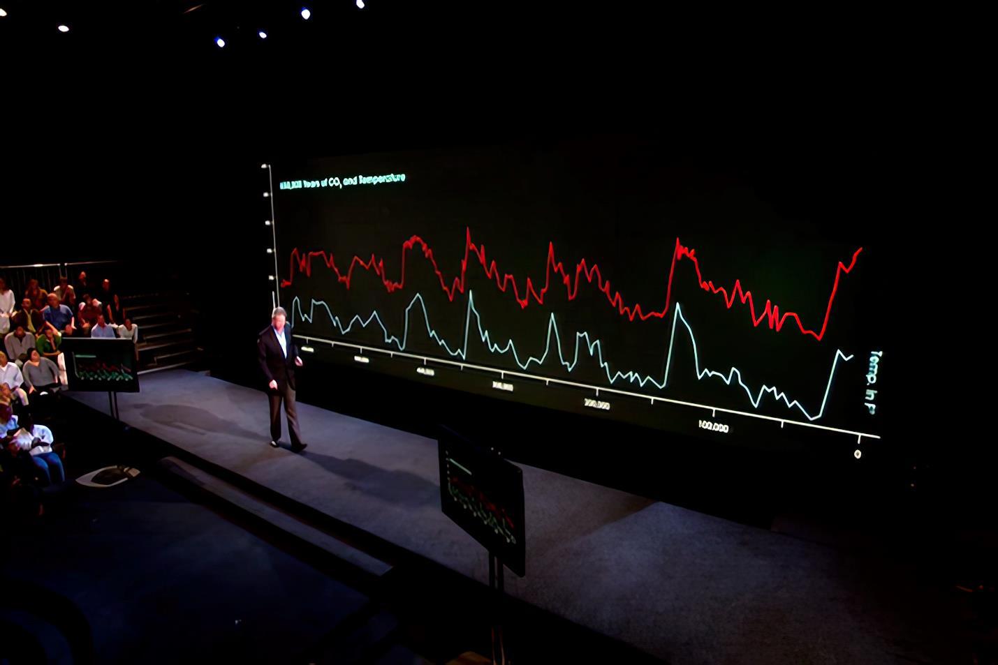
If you do not recall the climate scientists raising these obvious questions, it is not your memory that is at fault. Their silence was deafening.
Mr. Gore’s graph (Fig. 7) extends back about 600 thousand years and shows some visual correlation between temperature and atmospheric CO2 content. A close correlation between X and Y could mean: (A): To some extent X causes Y; (B): To some extent, Y causes X; (C) To some extent, both X and Y are caused by something else; or (D) the correlation between X and Y is accidental.
By contrast, Figure 8 extends back 600 million years and shows no correlation between the two quantities.

Figure 8: Long-term lack of correlation between temperature and CO2 concentration [4]
We will later show a published graph that pretends to show a correlation by using the logarithm of the CO2 concentration, which appears to shrink its variability.
Laboratory Measurements of GHG properties
So, the amount of IR emitted to space is less than the amount of IR emitted from the surface and also has a different spectrum. We naturally expect that the probability of absorption of IR must depend upon the intensity of IR, the wavelength, and the amounts of each greenhouse gas present in the air. But the property of the particular GHG at that particular wavelength that describes the likelihood of interaction is a cross-sectional area called the cross-section.
Imagine some gas X in a tube of cross-sectional area A and length L. There is no other gas in the tube, and the pressure is a tiny fraction of atmospheric pressure. There are N molecules in the tube, each posing a cross-sectional area, the cross-section , as shown in Figure 9. The molecules are represented as circles, but our experiments can only define the area , not the shape. With no changes to the tube or the gas in it, as an educational venture, we will do several gedanken experiments. An eyeball estimate would say that the little circles in Figure 9 occupy about 5%10% of the area.
9
Our first experiment will be to send a stream of (say) argon atoms into the tube at some velocity. What we will look for is a reduction in the stream at the exit end. Perhaps the stream becomes reduced by 10%.
Now, we will send in argon atoms that have high enough kinetic energy that they can ionize the molecules. Perhaps we will produce one ion for every 100 argon atoms entering the tube.
For another experiment, we will send in a beam of infrared radiation of some wavelength. For this wavelength, the intensity of the IR beam is reduced by one part in 10,000.
For another experiment, we will send in a beam of infrared radiation of some other wavelength. For this wavelength, the intensity of the IR beam is reduced by one part in 500
The lesson here is that there is no such thing as “the size of the molecule.” There is only an apparent size that depends on what experiment we perform.
For this reason, scientists measure a cross-section (a cross-sectional area; shape not defined) signified by the in Figure 9, and the cross section will be specified for each exact process. In Figure 9, there are N targets, each of cross-section , so the probability of the specified interaction is simply
You make measurements of probability of interaction and the number of targets per unit area of the tube. Do the simple arithmetic and you have measured the cross-section for that kind of interaction.
Figure 10 shows the measured IR absorption cross-section from the HITRAN database. The measurements cover a range from 2 10–26 cm2 to 5 10–18 cm2 (the “15-micron peak” at around 670 cm–1), a factor of 250 million. Needless to say, the measurements necessarily involved a wide range of experimental conditions.
The HITRAN data have been used by van Wijngaarden and Happer to calculate the effects on the IR spectrum from the equator to the poles and from the surface to the top of the atmosphere.

Now compare the size of the CO2 molecule (4-5 10–16 cm2 as it would be determined by its density as dry ice or by small-angle scattering experiments) with the IR cross-sections, as sketched in Figure 11. The largest IR cross-section is 5 10–18 cm2, only about 1% of the “size” of the molecule itself. Figure 10 shows measured cross-sections that are only a millionth as large as the largest cross-section.

Atmospheric CO2
Now we’ll discuss the effectiveness of CO2 as an IR absorber. It is best expressed by the mean free path, mean which turns out to be calculable from the absorption cross-section (to stay with international standards, we use square meters, not cm2) and the number density n (the number of molecules per cubic meter)
(4)
In the atmosphere at sea level, there are about 2.5 1025 molecules of air per cubic meter. Given that there are about 400 CO2 molecules per million of air molecules, then the value of n for CO2 is 1022 molecules/m3. Therefore mean at that high peak at atmospheric pressure is
In other words, at our present CO2 concentration, IR at about 670 cm–1 will travel only about 20 cm before being absorbed.
By contrast, around 570 cm–1, the cross-section is about 5 10–23 cm2 (5 10–27 m2), which is 5 factors of 10 smaller than at the peak, so the mean free path is 100,000 times as far 0.2 m 105 = 20,000 m or actually, quite a bit greater, since the atmosphere is very thin up there. (The peak of Mt. Everest is about 10,000 m above sea level, and the air pressure is about 1/3 of sealevel pressure.) The point is that IR of that wavelength is very unlikely to be absorbed in the atmosphere.
It would appear that the way to calculate the greenhouse effect for each gas would be to calculate the probability of IR of each wavelength to be captured before getting to space. In fact, that seems to havebeen thethinking oftheIPCC whentheypublishedtheirfirst Assessment Report in 1990. They published a graph (Fig. 12) which clearly shows the very strong absorption of the (near) 667 cm–1 line, with none of it going to space. By the time the Sixth Assessment Report (2021), the total number of IR spectra going to space published by the IPCC (either theoretical or measured) was exactly one the one in 1990 and it was wrong on two counts.
A: It disagreed with data that had already been taken twenty years earlier of the IR spectrum going to space by the Nimbus satellite (see Fig. 13).
B: It apparently assumed that the interaction between molecules and IR is not a one-anddone phenomenon.

Figure 12: Spectrum of IR emitted to space calculated incorrectly by IPCC [2]. It is the ONLY spectrum published in any of IPCC’s six Assessment Reports (1990 through 2021).
Figure 13 shows that the intensity of IR reaching outer space taken by the Nimbus satellite flying over Guam [5] In that 670-700 cm–1 band the intensity does not go to zero as the IPCC calculated in 1990, or as one would suspect from the fact that the mean free path of the 15-micron line is a mere 20 cm. In fact, the existence of that sharp peak in Figure 13 indicates that CO2 in the upper atmosphere is radiating strongly. A good absorber is a good radiator and conversely But why the radiation to space at that 670 cm–1 line?

Figure 13: Infrared emission to space measured by Nimbus satellite flying over Guam in 1970 [5]
Dynamics of molecular collisions
Molecules in the atmosphere are a tiny fraction of a millimeter apart, and they travel at roughly the speed of sound. Not surprisingly, collisions are extremely frequent. If a GHG molecule absorbs some IR, it converts all of the IR’s energy to internal rotational & vibrational energy modes. It can shed that energy by emitting IR or by being hit by another molecule (probably nitrogen or oxygen) in which case the energy thus becomes shared and very slightly heats the region.
Now imagine a GHG molecule being slammed by another molecule. The energy from the collision can be absorbed into an internal energy state that can emit IR. The molecule might emit IR or it might lose its excess energy through another collision. Non-GHGs (primarily nitrogen and oxygen) also have rotational and vibrational energy states that get excited and de-excited by collisions, but they neither absorb nor emit IR because these homonuclear molecules do not have a “handle” (technically, dipole moment) that allows interaction with IR.
There is thus a dynamic interplay going on everywhere in the atmosphere from the surface to the top of the atmosphere, and from the equator to the poles. At every altitude, every latitude, every temperature and every pressure, there are always collisions exciting and de-exciting
wavelength-dependent energy states, and always some IR is being absorbed and some IR is being emitted.
The generic field of interaction between IR and molecules is called molecular spectroscopy, and it involves both quantum-mechanical calculations and precision measurements.
In the atmosphere, those molecules interact with other molecules and IR in ways that depend on the temperature and the pressure. The kinetic energies of the molecules and the Doppler effect are temperature dependent. The closeness of molecules to one another affects the energies of excited states, hence there is so-called pressure broadening of spectral lines. The generic field of these interactions is called statistical mechanics
Absorbers & Radiators
There is a general principle pertaining to these GHG molecules: A good absorber is a good radiator. What is implied, but not often elucidated, is that this principle applies on a wavelengthby-wavelength basis. CO2 is a great IR absorber at ca. 670 cm–1 (ca. 15-micrometers wavelength) and agreat emitter(radiator)at thatsamepartofthespectrum, but it is averypoor absorber/emitter at 500 cm–1 (20 micrometers).
Just as the absorption of IR at a given wavelength is proportional to both the number of molecules per unit volume (n = N/V) and the absorption cross-section , the probability of emission at that wavelength is proportional to the same product, n.
To emphasize the point, notice that the peak in the CO2 spectrum at about 670 cm–1 (see Fig. 10) would imply (in the one-and-done absorption model) that there would be no IR of that wavelength going to space, as shown in IPCC’s only published spectrum (Fig. 12); however that absorption peak shows up as a peak in the emission spectrum to outer space measured over Guam in 1970 (Fig. 13). Even at the cold high altitude, collisions are kicking CO2 into excited states that radiate IR, in this case to outer space.
Surface IR Emission
We noted above that solid materials have energy levels so close together that they emit IR photons with a continuum of photon energies. The spectrum is known as the blackbody spectrum, and there is an equation derived in 1900 by Max Planck that is applicable to distant stars, molten lava in a volcano, hot pokers, your forehead, a block of ice, and a block of dry ice, to name a few. Needless to say, the spectrum is temperature-dependent, but the general shape of the curve is always the same. (See the smooth curves in Fig. 13.)
The smooth curves in Figure 13 were calculated from Planck’s formula. The important thing about such spectra is the area beneath the curve, say between two points on the horizontal axis. For example, consider the range between 600 cm–1 and 800 cm–1. The area beneath the jagged curvebetweenthosetwo numbersrepresentstheamountofIRpowerpersquarecentimeter emitted to space. The area beneath the 300 K curve between 600 cm–1 and 800 cm–1 represents the amount of IR power per square centimeter that would be emitted to space in that band by a 300-K surface if there were no GHGs (in this case, CO2 and H2O) there to interact with the IR. The area between those two curves is the net amount of IR absorbed per square centimeter.
For a blackbody, the total amount of power emitted per unit area is the area under the entire curve, and there is a simple formula for it called the Stefan-Boltzmann law:
Inthis case,theformulais expressedin Système International units:powerin watts, area in square meters, and absolute temperature in kelvins (K, not ºK). Figure 1 shows the IR emission from the surface to be 398 W/m2 (the negative sign merely meaning that heat is leaving the surface). By the Stefan-Boltzmann equation, this amount of radiation comes from a surface of 289.45K (16.3ºC, 61.3ºF) [The range of 395 to 401 corresponds to a temperature range of 289K to 290K.]

[Aside: There are more quantities needing symbols than there are letters in the Roman and Greek alphabets combined. The constant in the Stefan Boltzmann law is not to be confused with the cross-section .]
Another look at Figure 13 reveals a “Theoretical” curve that is a very good match to the data, except that the theory did not account for ozone (O3) in the atmosphere. The theoretical curve was calculated from the IR spectra of the GHGs, primarily H2O and CO2, so we should have a look at what is involved.
IR properties of GHGs
The present CO2 concentration is about 400 molecules of CO2 per million molecules of air (400 ppmv is thestandardnotation). But let’sstart with only 10 ppmv. Theonly partofthe IR spectrum that matters (Fig. 10) is a very narrow region centered around that peak at 670 cm–1; for the rest, the mean free path at that low concentration is so great that IR from the surface escapes to space. But in that part of the spectrum, there is near certainty that the IR is absorbed. Now increase the CO2 concentration to 20 ppmv and you easily increase the absorption. After a while, the effect is largely saturated. Add more CO2 and you widen the absorption curve a little, but the cross-section is so small that it has little effect.
Figure 14 shows the results carried out with the HITRAN data from Figure 10 in units of net suppressed IR flux (in W/m2) versus CO2 concentration. By about 20 ppmv way over at the left CO2 keeps about 15 W/m2 from going to space. To block the next 15 W/m2 from going to space requires adding 19 times as much CO2 (380 ppmv), reaching our present 400 ppmv and 30 W/m2 of net blockage by CO2. Doubling the present amount will increase the effect only 3 W/m2 .

In IPCC’s Third Assessment Report (2001) [6], they give three formulas for calculating the “radiative forcing” (i.e., increase in ability to block IR) for CO2, all of which are in reasonable agreement, and all of which are based on the IR spectrum of CO2 known at the time (and probably using the red lines of Figure 10, as an approximation). The top formula yields 3.7 W/m2 for doubling of CO2, which is 20% higher than Happer and van Wijngaarden get with the best spectral data. My preference is for the result based on HITRAN, but, as we shall soon show, both results lead to the same overall conclusions.

Figure 14: Net IR blockage (seen from top of atmosphere) by CO2 versus CO2 concentration, adapted from van Wijngaarden & Happer [1].
The Greenhouse Effect in watts per square meter

The term greenhouse effect has been used variously (A) as a descriptive about what happens to IR in the atmosphere; (B) as a quantitative term representing the amount of IR absorbed by the surface from the atmosphere (345 W/m2 in the drawing to the right); and (C) by the IPCC in its Sixth Assessment Report (2021) as a quantitative term representing the difference G between the amount of IR emitted by the surface and the amount of IR emitted to space ((398 – 240 = 158) W/m2 in the drawing). Now we can construct a heat flux equation that applies to all equilibrium situations (either on the earth or on any body with no peculiar heat sources orbiting any star anywhere). We combine Equation 2 with IPCC’s definition of G, the greenhouse effect to get:
Equation 7 has four variables. Let us presume for the moment that both the solar flux at orbit and the albedo remain constant, i.e., the left side of Eq. 7 remains constant. It follows that the right side must also remain constant. Therefore, if the greenhouse effect G changes, then there must be a change in the surface temperature such that the change in IR from the surface exactly balances the change in G
In IPCC literature, they refer to “radiative forcing” to changes in the radiative quantities meaning changes in solar flux, changes in reflected solar flux (due to changes in aerosols, land use, etc.), and changes in the greenhouse effect. Using to represent changes, we can rewrite Eq. 7 as
Or more simply as
At present surface temperature, an increase of 1ºC causes the surface to increase its emission by 5.47 W/m2
IPCC scenarios
Let us begin with IPCC’s Third Assessment Report (TAR). Figure 6.6 of that publication gives the total radiative forcing from all causes, 1750 to 2001, as 2.43 W/m2. The Summary for Policy Makerssays thatthe measuredtemperature change,1860 to 2001,is 0.8ºC. Therefore,theincrease in surface IR emission must be 4.4 W/m2, fully 2 W/m2 more than the forcing can account for.
IPCC’s “most likely” temperature rise to occur with a doubling of CO2 concentration (in almost all Assessment Reports is 3ºC, which would cause an increase in surface IR emission of 16.4 W/m2. How that is to be caused by CO2’s radiative forcing of 3 W/m2 (3.7 W/m2, according to IPCC) is a bit of a mystery.
The most recent of IPCC’s Assessment Reports is AR6, published in 2021. They refer to various scenarios as SSPx-y, where ‘SSPx’ refers to the Shared Socio-economic Pathway, one of 5 general expectations of CO2 emissions from now until 2100. Within each SSP there are subscenarios about things like methane (CH4) emissions, land use changes, and so forth, with special emphasis on total radiative forcing by 2100 of 1.9, 2.6, 4.5, 7.0, and 8.5 W/m2 Figure 15, from AR6, shows some representative SSPs, with IPCC’s low-contrast microfont scales and labels made legible.

Figure 15: Shared Socio-economic Pathways (SSPs) from IPCC’s Sixth Assessment Report [7], showing various CO2 emission scenarios.
IPCC’s predicted temperature rises by the 2080-2100 time period for the scenarios in Fig. 15 are shown in Figure 16. The first bar shows the total temperature rise by 2100, and the 2nd shows the contribution due to CO2. The third bar shows the contribution from other GHGs, and the last shows the (negative) contribution from changes in albedo. What the five charts have in common is that the major amount of temperature increase is from CO2, with other GHGs contributing about 40% as much as CO2 does, and all show an increase in albedo (meaning a decrease in absorbed solar energy).

Figure 16: IPCC’s calculated temperature consequences from 5 different SSPs in the Sixth Assessment Report [7].
Let us take the example of SSP3-7.0 because it corresponds to CO2 approximately doubling by the end of the century. Figure 17 shows that case (made legible) with some annotation. The vertical axis shows the predicted temperature rise, and I have added the corresponding increase in surface IR emission calculated from the Stefan-Boltzmann law. For this case, the total forcing that is, the total increase in the ability to block IR from going to space is 7.0 W/m2. By contrast, the increase in IR emission occasioned by the predicted increase in temperature is 20 W/m2. How is that possible?

17
It takes considerable imagination, looking at CO2 concentration and temperature in Figure 8, that the two quantities are correlated. However, the temperature rise is supposedly dependent upon the logarithm of the CO2 concentration, which has considerably less variation than the CO2 concentration itself. Judd et al [8] do not use the term logarithm in their text, but they plot the temperaturereconstructionversusthe logarithm oftheCO2 concentration, presumably recognizing that the forcing is proportional (over the range) to ln(C/C0), as noted in the section IR Properties of GHGs. However, their graph (see Fig. 18) does not have a forcing scale. Notice that in Figure 18 a radiative forcing scale has been appended.
Another scale that should have been in the original is the increase in surface radiation due to increased surface temperature, calculated from the Stefan-Boltzmann law. That scale is now appended in Fig. 18. Notice that the entire change in CO2 radiative forcing, from the least CO2 to the most, is 12 W/m2. By some feat of magic, that is supposed to suppress a total increase in surface IR emission of 140 W/m2. What’s a factor of twelve among friends?

18
et al say [8]:
There is a strong correlation between atmospheric carbon dioxide (CO2) concentrations and GMST [Global Mean Surface Temperature], identifying CO2 as the dominant control on variations in Phanerozoic global climate and suggesting an apparent Earth system sensitivity of ~8°C.
Atmospheric CO2 exerts a dominant control on GMST, both today and in the geologic past.
… [Temperature reconstruction] PhanDA GMST exhibits a strong relationship with atmospheric CO2 concentrations (Fig. 4), demonstrating that CO2 has been the dominant forcing controlling global climate variations across the Phanerozoic. (Emphasis added.]
No, Judd et al, you just proved that CO2 is a minor contributor to the temperature rise.
Measured Heat Balance
Refer back to Equation 7 which relates the surface temperature to the solar flux, the albedo, and the greenhouse effect G. The Clouds and the Earth’s Radiant Energy System (CERES) was initiated to study the earth’s heat balance. They concluded [9] that there is an imbalance (EEI, Earth’s Energy Imbalance), with a decadal increase amounting to 0.47 W/m2, caused by an increase in Absorbed Solar Radiation (ASR) of 0.73 W/m2 with a decrease in Outgoing Longwave Radiation (OLR, a.k.a., outgoing IR) (See Fig. 19). They concluded [9]:
• The EEI trend is primarily associated with an increase in absorbed solar radiation (ASR) partially offset by an increase in OLR.
• Large ASR trend primarily driven by reductions in low and middle clouds.
Translation: The warming trend since 2000 is caused mostly by a decrease in albedo, not repeat NOT by an increase in the greenhouse effect due to CO2.

Figure 19: Trends in watts per square meter per decade from Absorbed Solar Radiation (ASR), Outgoing Longwave Radiation (OLR), and Net effect from the CERES project [9]. In the CERES notation, outgoing longwave radiation is negative, and the negative OLR trend in this table means an increase in OLR, as noted in their conclusions listed above.
Conclusions
• At equilibrium, the amount of heat radiated to outer space equals the amount of heat absorbed from sunlight.
• The amount of IR emitted to outer space is less than the amount of IR emitted by the surface, and the spectrum of IR emitted to space is a jagged one, unlike the smooth spectrum of IR emitted by the surface. The greenhouse gases in the atmosphere, H2O, CO2, O3, and others are responsible for those differences.
• About 20% of the greenhouse effect is due to CO2; most of the rest is due to H2O. However, a The warmth of the surface is not due to atmospheric pressure; however, the decrease in temperature with altitude (the lapse rate) is due ultimately to the decrease in pressure with altitude.
• The science behind the greenhouse effect is molecular spectroscopy, including quantum mechanics and statistical mechanics, subjects that are not in the climate science curriculum
• Predictions made by climate models invariably overestimate future temperatures; in all cases (no exceptions!) the increase in surface IR emission far exceeds the radiative forcing that supposedly suppresses that radiation.
• The CERES project, specifically designed to measure the heat balance of the earth, has found that the present imbalance (leading to warming) is primarily caused by a decrease in albedo, NOT by the increase in atmospheric CO2.
• The CERES project specifically notes an increase in outgoing IR.
References
[1] W. A. van Wijngaarden and W. Happer, “Dependence of Earth's Thermal Radiation on Five Most Abundant Greenhouse Gases,” arXiv:2006.03098v1 4 June 2020
[2] IPCC’s First Assessment Report, 1990, https://www.ipcc.ch/
[3] Gregory Wrightstone, “Inconvenient Facts: Global Warming the Cold Hard Facts,” http://co2coalition.org/, 3/10/2021
[4] Gregory Wrightstone, “Virgina and Climate,” http://co2coalition.org 8/5/2023
[5] “The Nimbus 4 Infrared Spectroscopy Experiment, June 1973, https://ntrs.nasa.gov/archive/nasa/casi.ntrs.nasa.gov/19730018587.pdf
[6] IPCC’s Third Assessment Report (2001), https://www.ipcc.ch/
[7] IPCC’s Sixth Assessment Report (2021), https://www.ipcc.ch/
[8] Judd et al., “A 485-million-year history of Earth’s surface temperature,” Science 385, eadk3705 (2024)
[9] Norman G. Loeb “Observational Assessment of Changes in Earth’s Energy Imbalance Since 2000,” https://ceres.larc.nasa.gov/documents/STM/202305/15_Loeb_Contributed_Science_Presentation_2023.pdf