II. A Cloud Thermostat Controls the Earth’s Climate, Not Greenhouse gasses! and
I. Climate change is a myth!
John F. Clauser, retired experimental and theoretical physicist, 2022 Physics Nobel Laureate, Climate Change Denier 817 Hawthorne Drive Walnut Creek, CA 94596, email: bobbi_john@jfcbat.com, website: johnclauser.com
Zoom Lecture May 8, 2024
Irish Climate Science Forum & CLINTEL
1
Part I. Climate change is a myth -1.
• The IPCC and its collaborators have been tasked with computer modeling and observationally measuring two very important numbers – the Earth’s so-called power imbalance, and its power-balance feedback-stability strength. They have grossly botched both tasks, in turn, leading them to draw the wrong conclusion.
• I assert that the IPCC has not proven global warming! On the contrary, observational data are fully consistent with no global warming. Without global warming, there is no climate-change crisis!
• Their computer modeling (GISS) of the climate is unable to simulate the Earth’s surface temperature history, let alone predict its future.
2
Part I. Climate change is a myth -2.
• Their computer modeling (GISS) is unable to simulate anywhere near the Earth’s albedo (sunlight reflectivity). The computer simulated sunlight reflected power and associated power imbalance error, are typically about fourteen times bigger than the claimed measured power imbalance, and about twenty five times bigger than the claimed measured power imbalance error range.
• The IPCC’s observational data are wildly self-inconsistent and/or are fully consistent with no global warming.
• The IPCC’s observational data claim an albedo for cloudy skies that is inconsistent with direct measurements by a factor of two. Alternatively, their data significantly violate conservation of energy.
3
Part I. Climate change is a myth -3.
• Scientists performing the power-balance measurements admit that the available methodologies are incapable of measuring a net power imbalance with anywhere near the desired accuracy. This difficulty is due to huge temporal and spatial fluctuations of the imbalance, along with gross under-sampling of the data.
• The observational data they report are self-inconsistent and are visibly dishonestly fudged to claim warming. The fudged final reported values, herein highlighted and exposed, are an example of the proverbial proliferation of bad pennies.
• NOAA’s claims that there is an observed increase in extreme weather events are bogus. Their own published data disprove their own arguments. A 100 year history of extreme weather event frequency, plotted frontwards in time is virtually indistinguishable from the same historical data plotted backwards in time.
4
Part I. Climate change is a myth -4.
• In Part II, I present the cloud-thermostat feedback mechanism. My new mechanism dominantly controls and stabilizes the Earth’s climate and temperature. The IPCC has not previously considered this mechanism. The IPCC ignores cloud-cover variability.
5
The IPCC’s two sacred tasks – both botched! -1
1. The IPCC and its collaborators have been tasked with computer modeling and observationally measuring two very important numbers – the Earth’s socalled power imbalance, and its power-balance feedback-stability strength.
2. The Earth’s net power imbalance is its sunlight heating power (its power-IN), minus its two components of cooling power - reflected sunlight and reradiated infrared power (its power-OUT).
3. Based on their claimed power imbalance and global-warming assertion, the IPCC and its collaborators assemble a house of cards argument that forebodes an impending climate change apocalypse/catastrophe.
4. Additionally, the IPCC and its contributors calculate the strength of naturally occurring feedback mechanisms that presently stabilize the Earth’s temperature and climate.
6
The IPCC’s two sacred tasks – both botched! -2
5. They claim only marginal effectiveness for these mechanisms, and correspondingly assert that there is a “tipping point”, whereinafter further added greenhouse gasses catastrophically cause what amounts to a thermal-runaway of the Earth’s temperature.
6. The IPCC scapegoats atmospheric greenhouse gasses as the cause of global warming, and further mandates that trillions of dollars must be spent to stop greenhouse gas release into the environment with a so-called “zerocarbon” policy.
7. The IPCC also mandates multi-trillion dollar per year geoengineering projects including Solar Radiation Management Systems to stabilize the Earth’s climate and CO2 capture projects to reduce the atmospheric CO2 levels.
7
The IPCC’s two sacred tasks – both botched! -3
8. I assert that the IPCC and its contributors have not proven global warming, whereupon their house of cards collapses.
9. My cloud thermostat mechanism’s net feedback "strength" (the IPCC’s 2nd sacred task to estimate) is anywhere from -5.7 to -12.7 W/m2/K (depending on the assumed cloud albedo, 0.36 vs. 0.8), compared to the IPCC's botched best estimate for their mechanisms of -1.1 W/m2/K. My mechanism’s overwhelmingly dominant strength confirms that it is the dominant feedback mechanism controlling the Earth’s climate.
10.Correspondingly, I confidently assert that the climate crisis is a colossal trillion-dollar hoax.
8
The IPCC’s basic argument is a flawed house
of cards: -1
1. The IPCC claims with great certainty that the Earth has a (proven) net power imbalance. It claims that there is more sunlight power incident on the Earth heating it, than there is lost power cooling it. The lost power has two forms reflected sunlight and reradiated far infrared radiation.
2. More power IN than power OUT defines global warming! The IPCC claims a net warming power imbalance!
3. Global warming leads to climate change.
4. Climate change leads to an increased frequency of extreme weather events and other bad phenomena.
5. An increased frequency of extreme weather events leads to global apocalypse and a climate crisis. NOAA claims to have observed an increase. (Their claims are visibly bogus.)
9
The IPCC’s basic argument is a flawed house
of cards: -2
6. The IPCC’s claimed net warming power imbalance is claimed to be caused by an atmospheric buildup of greenhouse gasses, especially of CO2.
7. Trillions of dollars must therefore be spent to limit, prevent, and reverse the atmospheric buildup of greenhouse gasses.
8. However, given that said claimed net warming power imbalance is not proven, and there is actually no global warming, then there is no crisis and the house of cards has collapsed.
9. I assert that the IPCC’s claimed net power imbalance is not proven, and that there is no crisis. The house of cards has indeed collapsed! The requested trillions of dollars are a waste.
10
The IPCC’s computer modeling uses flawed physics to estimate the Earth’s temperature history -1
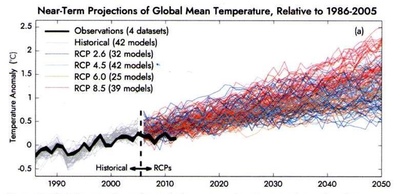
• The above graph is copied from [AR5, (IPCC, 2013) Fig 11.25].
• It shows the IPCC’s CMIP5 computer modeling of the Earth’s temperature “anomaly”. The various computed curves display the earth’s predicted (colored) and historical (gray) “temperature anomaly”.
• The solid black curve is the observed temperature anomaly.
11
The IPCC’s computer modeling uses flawed physics to estimate the Earth’s temperature history -2
(Repeat 1)
• Note that all 40+ models are incapable of simulating the Earth’s past temperature history. The total disarray and total lack of reliability among the CMIP5 predictions was first highlighted by Steve Koonin (former White House science advisor to Barack Obama) in his recent book- Unsettled? What climate science tells us, what it doesn’t, and why it matters.
• Something is obviously very wrong with the physics incorporated within the computer models, and their predictions are totally unreliable.
12
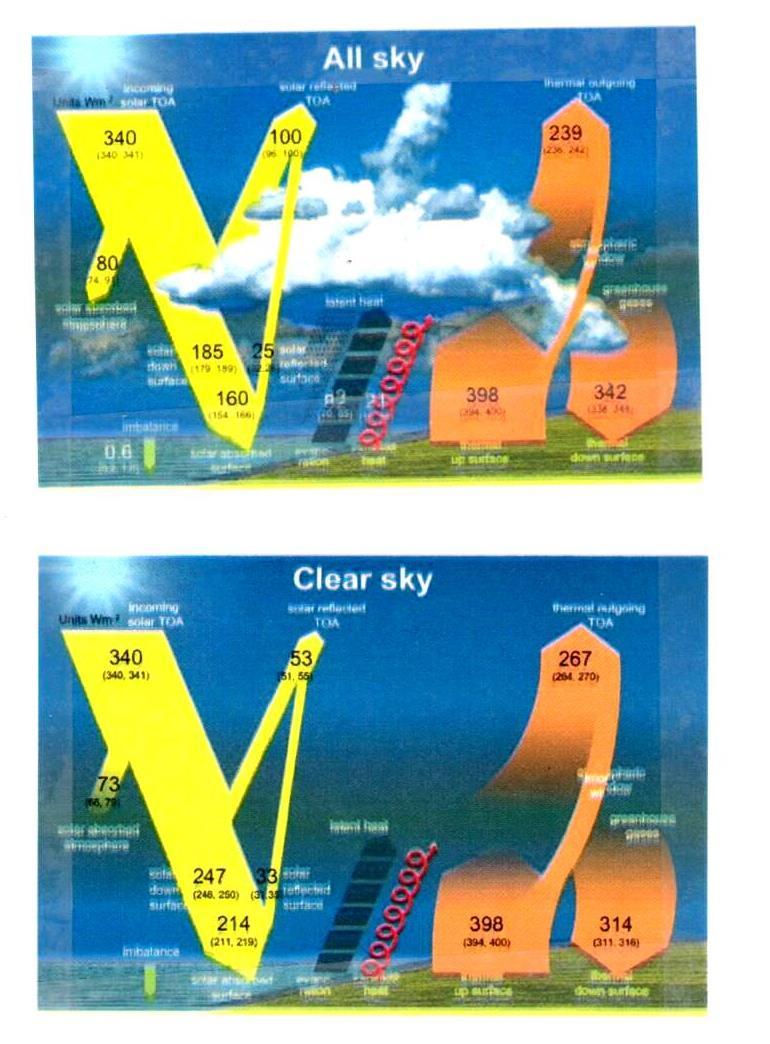
The IPCC’s computer modeling uses flawed physics to estimate the Earth’s albedo -1
Outgoing Shortwave Radiation (W/m2)
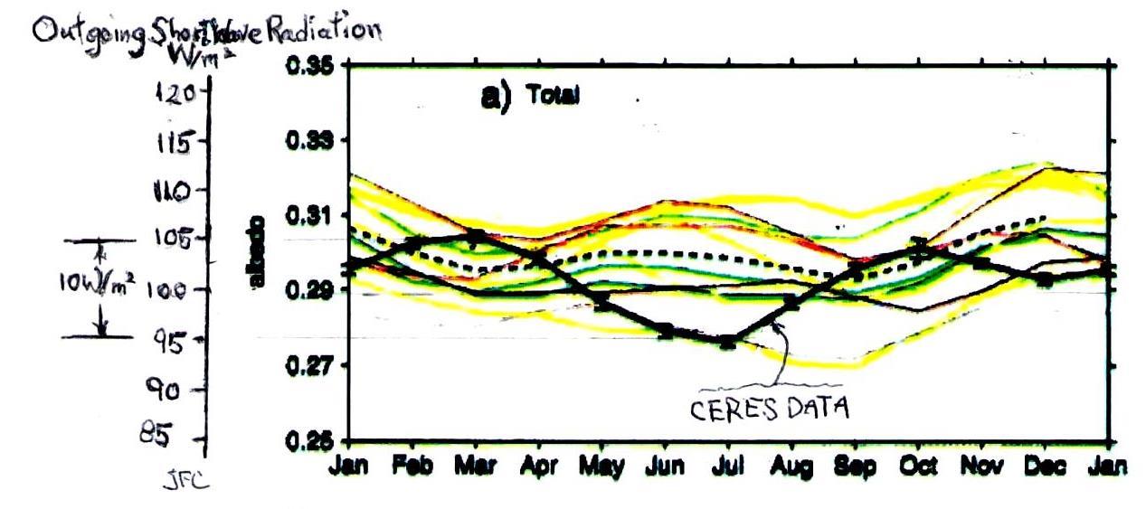
CERES
Data
• Albedo is the fraction of sunlight power that is directly reflected by the Earth back out into space. (OSR=100 W/m2 portion of power-OUT)
• The above Figure, copied from Stephens et al. (2015), shows the IPCC’s CMIP5 computer modeling (colored curves) of the Earth’s mean annual albedo temporal variation. The solid black curve is the Earth’s albedo measured by satellite radiometry. (The variation is not sinusoidal.)
13
albedo 10 W/m2
The
IPCC’s computer modeling uses flawed physics to estimate the Earth’s albedo -2
• The added scale shows the associated reflected sunlight power. It assumes a constant solar irradiance – 340 W/m2 .
• Note that the IPCC’s computer modeling is grossly incapable of simulating the observed Earth’s reflected power, and especially incapable of simulating that power’s dramatic temporal fluctuation.
14
Data albedo 10 W/m2 (Repeat 1)
Outgoing Shortwave Radiation (W/m2) CERES
The IPCC’s computer modeling uses flawed physics to
estimate the Earth’s albedo -3
Outgoing Shortwave Radiation (W/m2)
• The actual power’s annual variation is actually much greater than is shown by this Figure by about 18 W/m2, due to the ellipticity of the Earth’s orbit and the associated sinusoidal temporal variation of the so-called solar constant.
15
albedo 10 W/m2 (Repeat
CERES Data
2)
The
IPCC’s computer modeling uses flawed physics to estimate the Earth’s albedo -4
Outgoing Shortwave Radiation (W/m2)
• Despite more than 10 W/m2 gross errors in the computer simulation’s calculated reflected power, as is shown on the Figure, the IPCC [AR6 (2021)] still claims that it has computer simulated and precisely measured this power, yielding an imbalance that is equal to 0.7 ± 0.2 W/m
16
2 . – Huh?
(Repeat 3)
albedo 10 W/m2
CERES Data
The IPCC’s observational data are consistent with NO global warming - 1
• Power-IN is the sunlight power incident on the Earth. The IPCC and climate scientists call it Short Wavelength (SW) Radiation. It is about 340 Watts per square meter of the Earth’s surface area. (It is not actually constant, but varies ± 9 W/m2.)
• Power-OUT has two components:
• One component is the sunlight energy that is directly reflected by the Earth back out into space, whereinafter it can no longer heat the planet. That component is claimed by the IPCC to be about 100 W/m2 .
• The other component is the far-infrared heat radiated into space by a hot planet. It is claimed to be about 240 W/m2 . The IPCC calls the farinfrared heat radiation component,Long Wavelength (LW) Radiation.
17
The
IPCC’s observational data are consistent with NO global warming - 2
• Measuring the power imbalance consists of measuring power-IN, measuring power-OUT and subtracting. Simple enough? Not really. The problem is that power-IN, and power-OUT are huge numbers, and that the difference between them is miniscule - 0.2% of power-IN. That miniscule difference is the net imbalance that is sought, both experimentally and theoretically. Unfortunately, it is so small that it is very difficult, if not impossible, to measure to the desired accuracy, 0.1 W/m2, or 0.03% of power-IN. It is much tougher to measure when power-IN and power-OUT are both also hugely varying in a seemingly random irreproducible fashion. Large variations occur both in time and in space over the surface of the Earth. As noted in a previous slide, this grossly under-sampled fluctuation is about 28 W/m2 , compared with the IPCC’s claimed imbalance, 0.7 ± 0.2 W/m2 .
18
The
IPCC’s observational data are consistent with NO global warming - 3
• A variety of methods has been employed to measure these powers. They include satellite radiometry, (the ERBE, and CERES Terra and Aqua satellites), ocean heat content (OHC) measured using the ARGO buoy chain and XBT water sampling by ships, and finally by ground sunlight observations using the Baseline Surface Radiation Network (BSRN).
• The various measured values are all in wild disagreement with each other. Importantly, none of the reported data actually show a convincing net warming power imbalance. Importantly, much of the reported data are totally fudged in a manner that dishonestly changes them from showing no warming to showing warming!
19
What is the basic power-imbalance calculation? It is really quite simple - 1.
Observers’ data are usually reported on a Figure that shows a map of the claimed power flow.
The imbalance is conventionally reported at the Top Of Atmosphere (TOA).
The three needed numbers are readily available from the top line of the power-flow diagram.
If you don’t believe my claims of fudging, it’s easy enough to freely download the articles, pull the numbers from the various power-flow diagrams, and verify the arithmetic yourself!
A typical calculation is shown on the next slide:
20
What is the basic
power-imbalance calculation?
It is really quite simple - 2.
A typical calculation is as follows: Incident ShortWave
Fudged arithmetic is highlighted in red on the next slides. (Follow the proverbial bad penny.)
+340 W/m2 ± σIN
reflected power -100 W/m2 ± σSW-OUT Outgoing
power -240 W/m2 ± σLW-OUT
σIMBALANCE σIMBALANCE = (σIN 2 + σSW-OUT 2 + σLW-OUT 2)1/2 . (RMS sum) RMS sum crosscheck: σIMBALANCE > σIN, σIMBALANCE > σSW-OUT, σIMBALANCE > σLW-OUT. no global cooling if IMBALANCE ≤ σIMBALANCE global warming if IMBALANCE > σIMBALANCE
21
power
Outgoing ShortWave
LongWave reemitted
Sum=Net “observed” power imbalance IMBALANCE ±
The earliest data are reported by Stephen’s et al. (1981) and Ramanathan (1987) - 1.
• Their results are based on only four partially analyzed months of observation by the ERBE satellite – (Apr. 1985, July 1985, Oct. 1985, Jan. 1986). (c.f. observed non-sinusoidal albedo annual oscillation.)
• Their resulting Top of Atmosphere net power imbalance results are as follows: Stephens et al. Ramanathan (1981) (1987)
• Both Stephens et al. and Ramanathan’s data are fully consistent with zero net global warming and/or cooling.
Incident ShortWave power (W/m2) +344 +340 Outgoing ShortWave power -103.2 -106 Outgoing LongWave power -234±7 -237 Net “observed” power imbalance +9 ± 10 0 jfc calculation +6.8 -3
22
The earliest data are reported by Stephen’s et al. (1981) and Ramanathan (1987) - 2.
• The 2003 US National Academy / National Research Council report “Understanding Climate Change Feedbacks (p.112)” cites the Ramanathan (1987) data, and comments that “The observations do not meet quality standards.”
23
Loeb et al. (2009, 2012) use OHC data to “adjust” Ramanathan’s (1987) numbers, to show a net warming power imbalance - 1.
• Loeb et al. (2012, p.111) admit ”A limitation of the satellite data is their inability to provide an absolute measure of the net TOA radiation imbalance to the required accuracy level.”
• Loeb et al. (2009, 2012) reanalyze and arbitrarily replace Ramanathan (1987)’s (very sparsely sampled) EREB satellite data with new values that now show a net global warming power imbalance.
• They obtain their new preferred data values by switching modality from satellite-radiometry data to ocean heat content (OHC) data (also very sparsely sampled) from the ARGO buoy chain, and from XBT ship-based bathythermograph manually sampled water temperature data.
• They base their action on a claimed increase in ocean heat content, as per speculation by Hansen et al, (2005, 2011).
24
Loeb et al. (2009, 2012) use OHC data to “adjust” Ramanathan’s (1987) numbers, to show a net warming power imbalance - 2.
• Unfortunately, the ARGO and XBT data have a woefully sparse area sampling, and much worse accuracy than Loeb et al. claim. Data gaps are filled using totally fabricated data by Lyman and Johnson (2008). (Data fabrication is one of our scientific little no-no’s.)
• Their resulting Top of Atmosphere net power imbalance results:
Remember this proverbial BAD PENNY. It will show up again and again, and again.
EREB OHC OHC satellite (2009) (2012) Incident ShortWave power (W/m2) +340 +340 Outgoing ShortWave power -107 -99.5 various Outgoing LongWave power -234.6 -239.6 ________ net power imbalance -1.6 + 0.9 +0.64 ± 0.11 (cooling) (warming) (warming) THE BAD
PENNY
25
Power imbalance analysis by Stephens et al. (2012) with grossly admittedly-fudged error estimates - 1
• Following Loeb et al., Stephens et al. (2012) also admit that satellite data are incapable of observing a net imbalance! The groups join forces and switch to the use of Ocean Heat Content (OHC) data, as per the suggestion by Hansen et al, (2005, 2011).
• Stephens et al. (2012) use OHC data and the Outgoing ShortWave power “adjustment” (fudge!) reported earlier by Loeb et al. (2009, 2012) to claim a net global-warming power imbalance (the BAD PENNY reappears!):
Incident ShortWave power (W/m2)
+340.2 ± 0.1
Outgoing ShortWave power -100.0 ± 2.0
Outgoing LongWave power -239.7 ± 3.3
Net “claimed observed” power imbalance +0.6 ± 0.4 recurring BAD PENNY (fudged warming) Actual summation & assoc. RMS error (jfc) +0.5 ± 3.9 (no warming)
26
Power imbalance analysis by Stephens et al. (2012) with grossly admittedly-fudged error estimates - 2
• Stephens et al.’s use of (visibly) incorrect arithmetic is yet another one of our scientific little no-no’s. RMS error sum crosscheck NG.
• Loeb et al. (2012)’s BAD PENNY error limits are increased from ± 0.11 to ± 0.4.
27
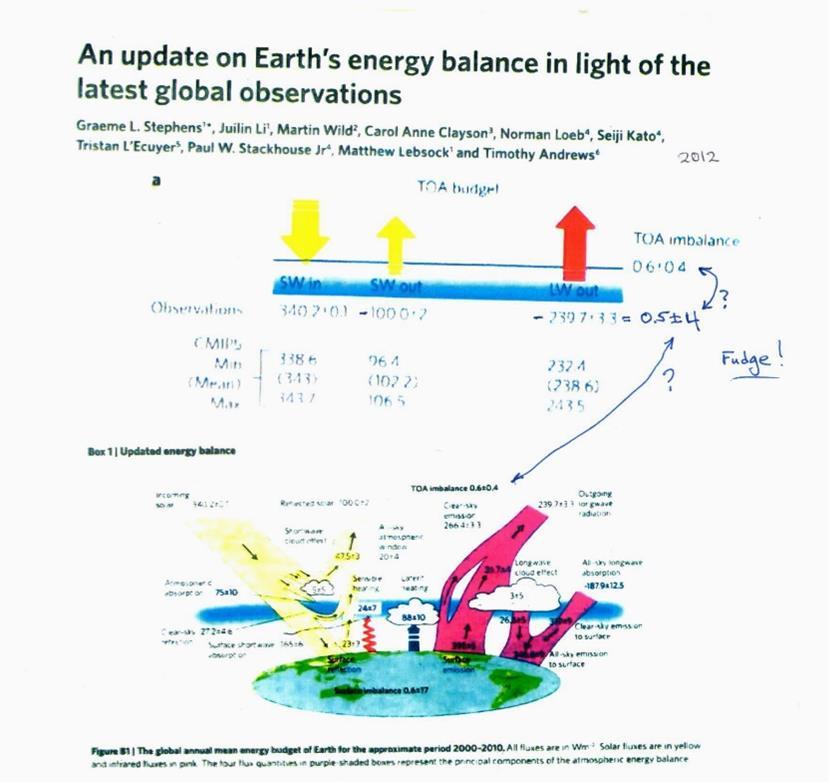
Stephens et al.
(2012)
power-flow diagrams show the fudged numbers
Figures 1 and B1 from Stephens et al. (2012), displaying the bad arithmetic and comparing it with the CMIP5 computer modeling.
28
L’Ecuyer et al. (2015) reanalyze the Ocean Heat Content (OHC) data and get different results and much larger error estimates than reported by Stephens et al. (2012)
• Following the Stephens et al. (2012) estimate of the Earth’s power imbalance based on OHC data, L’Ecuyer et al. (2015) revise Loeb et al.’s (2009, 2012) ocean heat content data analysis.
• They correspondingly revise upwardly the (fudged) power imbalance error limits offered by Stephens et al. (2012). They do, however, provide their own “adjustments”, that they instead call constraints.
unconstrained constrained Incident ShortWave power (W/m2)
± 0.5
± 0.1
(no warming) (no warming)
+340.0
+340.2
-102
-238
-238
Net
0 ± 5.0 0 ± 3.5
29
Outgoing ShortWave power
± 4 -102 ± 4 Outgoing LongWave power
± 3
± 2
“observed” power imbalance
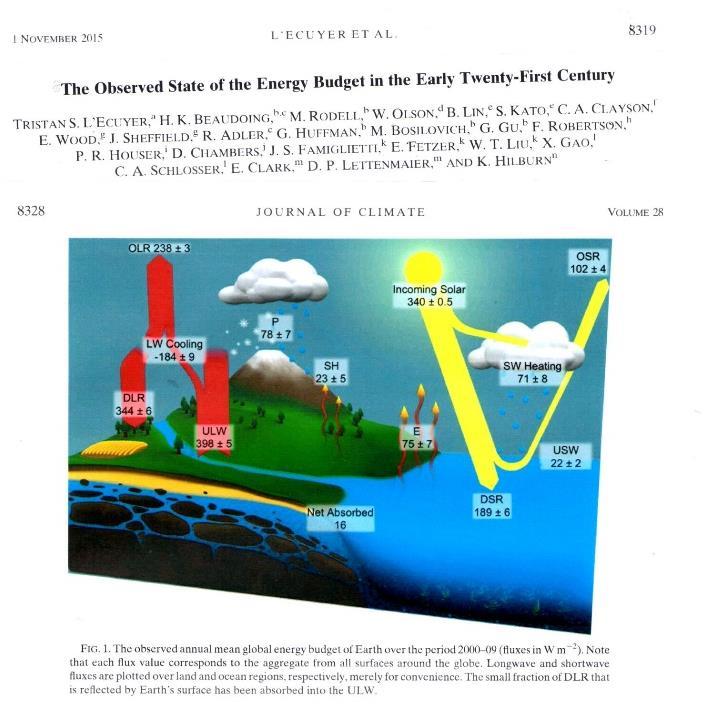
30
Power flow diagram from L’Ecuyer et al. (2015, Fig.1.)
Critiques by Trenberth et al. (2010, 2014) - 1
• Satellites measure the Top of Atmosphere energy balance, while Ocean Heat Content data apply to the surface energy balance. One may legitimately mix power-flux data at the two different altitudes, if and only if one fully understands all of the power-flow processes in the atmosphere that occur between the surface and the Top of Atmosphere. If the latter requirement is not true, then one ends up with an “apples to oranges” comparison.
• Trenberth et al. (2010, 2014) are highly critical of Loeb, Stephens, L’Ecuyer, and Hansen’s claimed “understanding” of the associated connection between the power flows at these two altitudes.
• Trenberth and Fasullo (2010) point to a huge “missing energy” indicated by the difference between the satellite data and the OHC data power-imbalance calculations, and specifically ask “Where exactly does the energy go?”
31
Critiques by Trenberth et al. (2010, 2014) - 2
• Hansen et al. (2011) dismiss Trenberth and Fasullo’s alleged missing energy as being simply due to satellite calibration errors.
• Trenberth Fasullo and Balmesada (2014) further note that despite various considerations of the surface power balance, significant unresolved discrepancies remain, and they are skeptical of the power imbalance claims.
• In effect, Trenberth et al. are the earliest “whistle blowers” to the abovementioned data fudges.
32
Stephens and L’Ecuyer (2015) together offer a mea culpa admission to having made an “unjustified, ad hoc” choice between OHC data and CERES satellite data, and miraculously now claim simultaneously both zero and +0.6 +/- 0.4 W/m2 power imbalance.
• In response to criticism by Trenberth et al. (2010, 2014), Stephens and L’Ecuyer (2015) together offer what amounts to a mea culpa article regarding the aforementioned data fudging. They admit that “adjustments” do need to be made to obtain agreement (closure) between satellite data and ocean heat content data, and that these “adjustments” are very much larger (by about 10 W/m2) than their claimed power imbalance, +0.6 +/- 0.4 W/m2 .
• Stephens and L’Ecuyer (2015) also admit that their choice of which data needs “adjustment” was made “in a totally ad hoc” fashion, and that “there is no real evidence to support one adjustment approach over the other”.
• Amazingly, Stephens and L’Ecuyer (2015) persist in reporting (in their abstract line 5) the power imbalance = 0.6 +/- 0.4 W/m2. (The infamous Loeb et al. (2012) global-warming BAD penny reappears again!).
OHC CERES (satellites)
Power imbalance reported (abstract line 5) +0.6 +/- 0.4 W/m2 (= warming)
Net “calculated” power imbalances (jfc) 0 ± 5.6 0 ± 5.6 (no warming) (no warming)
ShortWave power (W/m
+340.0 ± 0.1 +340.0 ± 0.1 Outgoing ShortWave power -102 ± 4 -100 ± 4 Outgoing LongWave power -238 ± 4 -240 ± 4
Incident
2)
33
Power imbalance analysis by Wild et al. (2019) and AR6 (2021) – imbalance and error bars fudged - 1.
• Wild et al. (2019) report new Clear sky (cloud-free-sky) measurements to the data set using ground sunlight observations via the Baseline Surface Radiation Network (BSRN).
• Wild et al. (2019)’s observational data claim an albedo for cloudy skies that is inconsistent with direct measurements by a factor of two, and/or significantly violates conservation of energy. (See energy conservation theorem Part II and Appendices A,B.) Their data require a cloudy-sky albedo ≈ 0.36, while direct measurements indicate a value ≈ 0.8.
• The Wild et al. (2019)’s diagram is copied directly by AR6 (2021), except for added fudges. The power fluxes and error bounds presented here are copied directly from the top lines of their nearly identical power-flow diagrams. The fudged power imbalances are copied directly from the associated lower lefthand corners.
34
Power imbalance analysis by Wild et al. (2019) and AR6 (2021) – imbalance and error bars fudged - 2.
Incident ShortWave power (W/m2) see note**
Wild et al. (2019) AR6 (2021)
± 0.5
± 0.5
(lower left hand corner of Figures) (warming) (strong warming)
Net “calculated” power imbalance (jfc) 3.5 ± 3.6 2.5 ± 3.0 (no warming) (no warming)
• The infamous Loeb et al. (2012) global-warming BAD PENNY reappears once again in Wild et al.(2019).
+340.5
+340.5
-98
-98.5
Outgoing LongWave power -239 ± 3 -239.5 ± 2.5 Power imbalance reported at bottom +0.6 +/- 0.4 +0.7 ± 0.2
Outgoing ShortWave power
± 2
± 1.5
35
Power imbalance analysis by Wild et al. (2019) and AR6 (2021) – imbalance and error bars fudged - 3.
• The arithmetically incorrect fudged numbers shown in red are the values reported at bottom of their power flow diagrams. My last line gives the correct summation.
• Wild et al. (2019) introduce an innovative technique for data fudging: The Incident ShortWave power reported by previous power-flow maps (e.g. by Stephens and L’Ecuyer (2015), is typically 340.0 ± 0.1 W/m2. Wild et al. (2019) and AR6 (2021) assume 340.0 ± 0.5 W/m2, round upwardly the center of their asymmetric error-limit range by +0.5 W/m2, and show both limits correspondingly rounded (upwardly) to the nearest whole number, as per 340 (340, 341) W/m2. Note that their upward rounding amount, +0.5 W/m2 , similarly shifts upwardly their calculated power imbalance by almost all of their reported net power imbalances, +0.6 +/- 0.4 and +0.7 ± 0.2.
36
Wild (2019, left pair) & AR6 (2021, p.934), right pair) power-flow diagrams.
37
NOAA’s scientific disinformation hoax asserting that the frequency of extreme weather events is increasing
• 2012, Physics Today article “Predicting and Managing Extreme Weather Events” – Earth’s climate is warming, and destructive weather is growing more prevalent. Coping with the changes will require collaborative science, forward-thinking policy, and an informed public.”
• Authors: Jane Lubchenco, undersecretary for oceans and atmosphere at the US Dept. of Commerce, and NOAA administrator, and Thomas Karl, Director of NOAA’s climatic data center and chair of the US Global Change Program.
38
NOAA’s disinformation hoax regarding an impending climate apocalypse
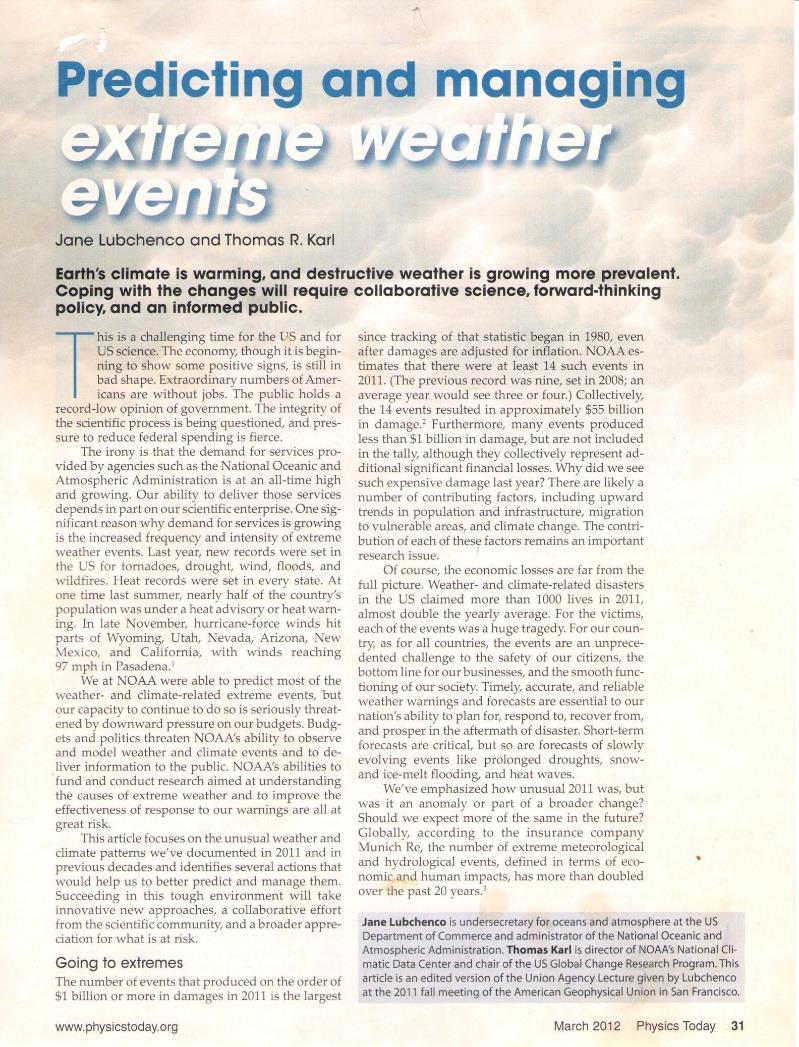
• The article asserts that there is an increase in the extreme weather event frequency that is associated with climate change in the three decades ending in 2012.
• The article presents data in their Fig. 2a displaying NOAA’s Weather and Climate Extremes Index. That index is NOAA’s numerical composite measure of the frequency of so-called extreme weather events, including hot-spells, cold-spells, droughts, floods, land-falling hurricanes, etc. (EF3+ tornado frequency is conspicuously absent from the list, presumably because it was actually decreasing. See Koonin, pp.124-125)
• The authors assert that their climate extremes index has “obviously” grown steadily over the last three decades. I assert here that their own data in their Fig. 2a disprove their own assertion.
39
Lubchenco and Karl’s Fig. 2a
40
The two graphs below are traced directly from Fig. 2a. They are identical, except that one is plotted left-to-right reversed, i.e. backwards with time increasing to the left. If you look carefully, you will see that they are mirror images. If you can’t tell which one of these graphs is correctly plotted and matches the one on the previous slide, and which one is time-backwards, I assert that their claimed recent increase in extreme weather-event frequency is not obviously indicated by their data, as they claim. Their claim is false! Are you really confidently willing to bet trillions of dollars that you can tell which one is correct? These data portend the impending apocalypse, so Lubchenko and Karl claim.
41
Part I – Conclusions - 1
1. The IPCC and its contributors claim the Earth has a net-warming energy imbalance. I show here that those claims are false.
2. The IPCC bases its claims on computer modeling of the Earth’s atmosphere, and on observational data from a variety of observational modalities. Both the computer models and the observational data are grossly flawed, and fudged.
3. The IPCC’s computer modeling and its predictions are totally unreliable. There is something clearly very wrong with the physics incorporated within these computer models. Since the computer models can’t even explain the past, why should anyone trust their prediction for the future?
4. Not one of the observational modalities for measuring the Earth’s power imbalance convincingly shows net global warming.
42
Part I – Conclusions - 2
5. I show where various observers and the IPCC have dishonestly fudged their reported data, and have dishonestly changed it from showing No Warming, to showing Warming. Crucially important data fudges are revealed here and highlighted in red. If you don’t believe me, check my arithmetic.
6. The IPCC and NOAA further claim that the purported power imbalance has already caused an increase in dangerous extreme weather events. NOAA’s own data disprove their own claims.
7. I thus offer Great News. Despite what you may have heard from the IPCC and others, there is no real climate crisis! The planet is NOT in peril!
8. The IPCC’s (and NOAA’s) claims are a hoax. Trillions of dollars are being wasted.
43
Part II – The cloud thermostat - 1
1. So what is really happening? Why is the earth’s climate actually as stable as it really is?
2. The cloud thermostat mechanism is clearly the overwhelmingly dominant climate controlling feedback mechanism that controls stabilizes the Earth’s climate and temperature. It thereby prevents global warming and climate change.
3. The cloud-thermostat mechanism provides very powerful feedback that stabilizes the Earth’s climate and temperature. It great strength obtains from the observed large fluctuation of the Earth’s power imbalance.
4. The mechanism gains its strength from the Earth’s observed very large cloud-cover variation. The power imbalance is actually observed to be continuously strongly fluctuating by anywhere between 18 to 55 W/m2 .
44
Part II – The cloud thermostat - 2
5. Clouds modulate the outgoing Shortwave power and therefore control the Earth’s power imbalance, minimally with a 18 W/m2 available power range (ignoring the added 18 W/m2 solar-constant variation), which is minimally 26 times the IPCC’s 0.7 W/m2 claimed power imbalance, and 45 times the IPCC’s ± 0.2 W/m2 power imbalance error range.
6. The above numbers use the IPCC’s assumed data parameters. With more realistic assumptions, the cloud-thermostat mechanism controls the Earth’s power imbalance with a 73 W/m2 available power range, which is 100 times bigger than the IPCC’s 0.7 W/m2 claimed power imbalance, and 180 times bigger than the IPCC’s ± 0.2 W/m2 power-imbalance total error range.
45
Part II – The cloud thermostat - 3
7. This seemingly random fluctuation of the power imbalance is not random at all, but is actually a crucial part of a thermostat-like feedback mechanism that controls and stabilizes the Earth’s climate and temperature. It is observed by King et al. (2013) and by Stephens et al. (2015) to be quasi-periodic,
8. Just like the thermostat in your home, the power-imbalance is never zero. The furnace or AC is always either ON or OFF. The thermostat simply modulates the heating/cooling duty cycle.
46
Features of the cloud thermostat mechanism
1. In preparation for the introduction of this model, I first describe important, underappreciated, but conspicuous properties of clouds - their variability and their strong reflectivity of sunlight (SW radiation).
2. I show that the cloud-thermostat mechanism involves the dominant (73%) use of sunlight energy by the planet.
3. I show that when the cloud-thermostat mechanism is viewed as a form of climate-stabilizing negative feedback, it is by far the most powerful of any such mechanism heretofore considered.
4. The IPCC estimates that the net stabilizing feedback strength or the Earth’s climate, including the destabilizing feedback strength of greenhouses is about -1 W/m2/ºC.
5. I show that the cloud thermostat feedback increases the net natural stabilizing feedback strength to about anywhere between -7 W/m2/ºC and -14 W/m2/ºC, depending on the assumptions used.
47
Some important properties of clouds
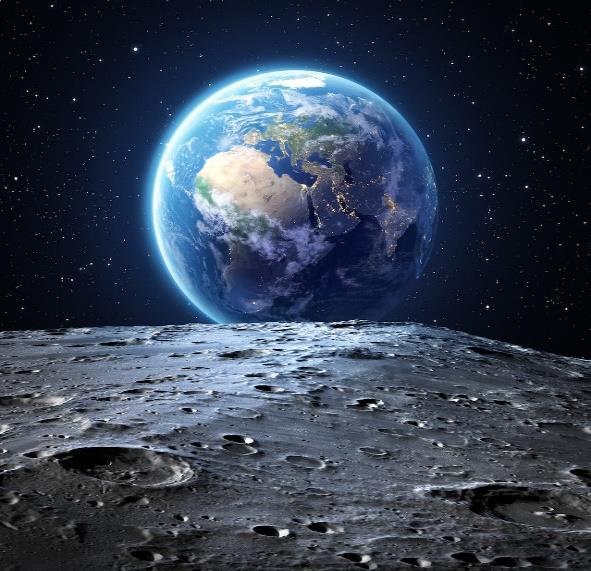
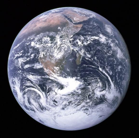
What does the Earth look like when viewed from space in sunlight?
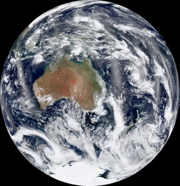
48
There are 5 important take-home messages to be gleaned from these satellite photographs.
1. Clouds reflect dramatically more sunlight than the rest of the planet does!
2. Clouds of all types appear bright white!
3. The photos (along with a large number of careful measurements) strongly suggest that the average cloud reflectivity (of sunlight) is about 0.8 – 0.9. (For comparison, white paper has a reflectivity of ≈ 0.99.) [Wild et al. (2019) claim that cloud reflectivity is 0.36.]
4. The rest of the planet appears much darker than the clouds. The average reflectivity of land (green and brown areas) and ocean (dark blue areas) is ≈ 0.16.
5. Cloud coverage area is highly variable over the Earth.
49
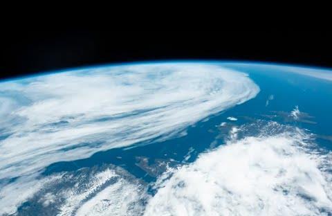
Clouds cast dark shadows.
• Clouds cast dark sharply-defined shadows on the surface below them. Just stand on a hillside or look down from an airplane on a partly cloudy day and watch the cloud shadows cast on the land below.
• Watch your solar-panel output when a solitary cloud passes in front of the sun. Typically, the output drops to 50% or less.
• Try reading a book indoors on a heavily overcast day without turning on the lights. You can’t. It’s too dark! Where did all of the missing sunlight go? Since water droplets negligibly absorb sunlight, the missing sunlight (typically 80-90% of it) got reflected back out into space.
50
What does sunlight mostly do when it reaches the Earth’s surface?
• It is commonly believed that sunlight that is absorbed by the Earth’s surface simply warms the surface. That may be true over land. But land represents only about 30% of the surface.
• Oceans cover 70% of the Earth’s surface. Correspondingly, about 70% of incoming sunlight falls on the oceans. Virtually all of the Earth’s exposed water surface occurs in the oceans.
• Following the AR6 power-flow diagram, 160 W/m2 is absorbed by the whole Earth, meaning that roughly 70% X 160 = 112 W/m2 is absorbed by oceans.
• The AR6 power-flow diagram indicates that 82 W/m2 is used for evaporating water, and not for heating the surface.
• Since clouds are mostly produced over the oceans (because that’s where the exposed water is), then 82/112 = 73% of the input energy absorbed by the Earth’s oceans is used, not for warming the Earth, but instead simply for making clouds.
51
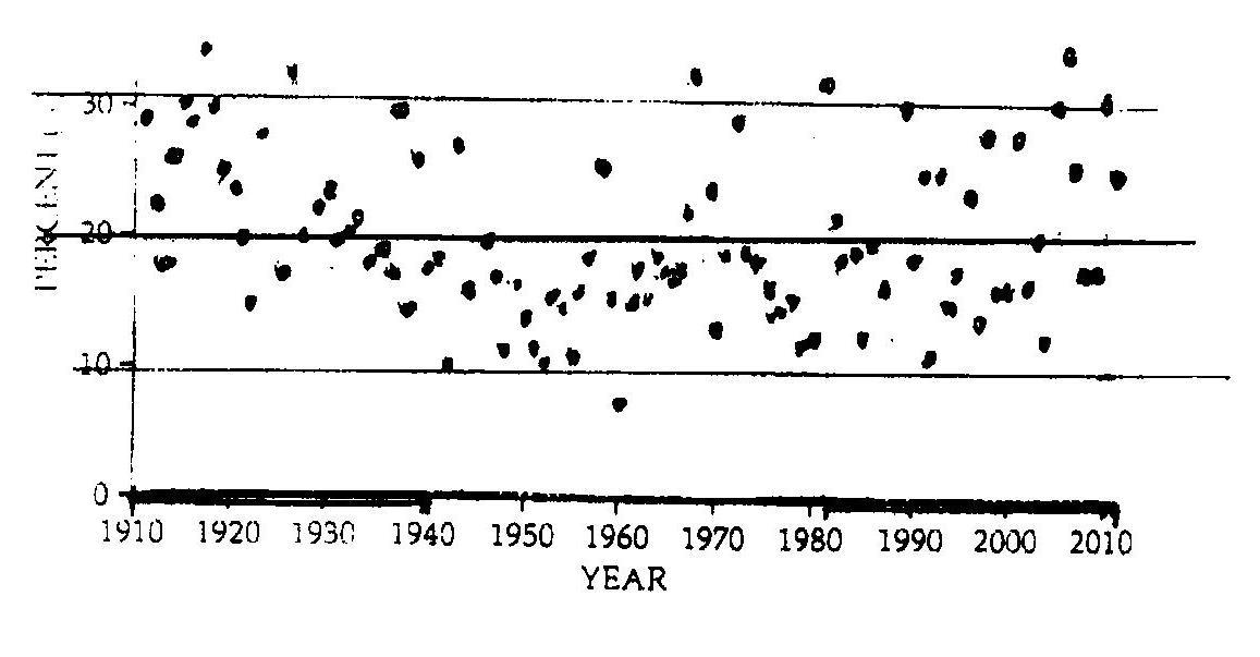
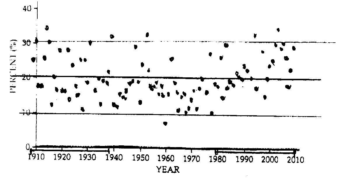
Satellite observations of cloud-cover fraction by King et al. (2013) -1.
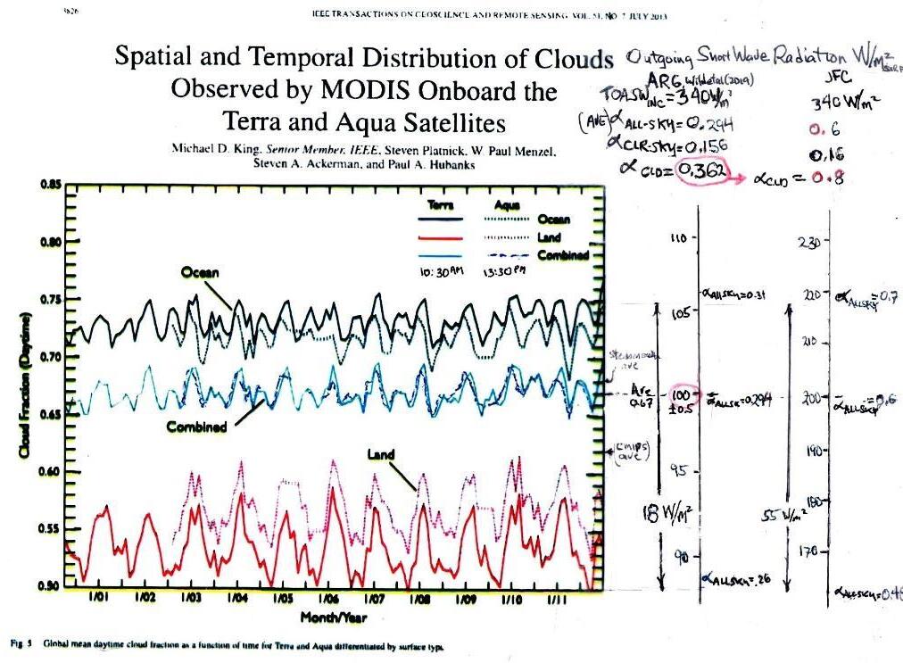
• King et al. (2013) analyzed more than 12 years of data from the CERES Terra and Aqua sun-synchronous satellites, and measured the daytime fractional cloud cover, over ocean, land, and combined.
• I have added Outgoing (reflected sunlight) SW power scales, assuming a constant solar input power, 340 W/m2 .
52
Satellite observations of cloud-cover fraction by King et al. (2013) -2.
• The left-hand scale uses the parameters from the 2021 AR6 report. It assumes an all-sky albedo = 0.3, and a clear-sky albedo = 0.16. Energy conservation (see Appendix B) further requires a cloudy-sky reflectivity (albedo) = 0.36. (an unreasonable value). On this scale, reflected SW power fluctuates by as much as 18 W/m2 .
53
Satellite observations of cloud-cover fraction by King et al. (2013) -3.
• The right-hand scale uses the same parameters, except that it assumes a cloudy-sky albedo = 0.8, as per the cloud photos and various measurements.
Reflected SW power then fluctuates by as much as 55 W/m2 .
54
Satellite observations of cloud-cover fraction by King et al. (2013) -4.
• The cloud-fraction variation is extremely strong and very rapid. The difference between the adjacent solid and dotted lines is the average everyday variation in only three hours – from 10:30AM to 13:30PM.
• Recall that the IPCC insists that the global average power imbalance is always precisely 0.7 ± 0.2 W/m2 .
55
Satellite observations of cloud-cover fraction by King et al. (2013) -5.
• The albedo fluctuation data presented by Stephens et al. (2015, see earlier slide), compared to this Figure, shows that the albedo fluctuation is due to cloud-cover fraction variation.
• Conclusion: Cloud-fraction variation, especially for clouds passing from ocean to land, strongly modulates the Outgoing sunlight power, and strongly affects the power imbalance.
56
My cloud thermostat model – how does it work-1?
1. Recall that the IPCC’s AR6 power-flow map asserts that 73% of the input energy absorbed by the Earth’s oceans is used, not for warming the Earth, but instead simply for evaporating seawater and making clouds, rather than for raising the Earth’s surface temperature. Recall that the Earth has a strongly varying cloud cover and albedo.
2. Temperature control of the Earth’s surface by this mechanism works exactly the same way as does a common home thermostat. A thermostat automatically corrects a structure’s temperature in the presence of varying modest heat leaks. For the earth, the presence of significant CO2 in the earth’s atmosphere, manmade or not, provides, in fact, a very small heat leak (at most, about 2 W/m2).
Note that, just like the Earth, the power imbalance for a thermostatically controlled system is never zero. It is always fully heating or fully cooling.
57
My cloud thermostat model –
3. How does the cloud thermostat work? When the Earth’s cloud-cover fraction is too high, then the earth’s surface temperature is too low. Why? Clouds produce shadows. Cloudy days are cooler than sunny days. A high cloud-cover fraction equals a highly shadowed area. With reduced sunlight reaching the ocean’s surface and lower temperature, the evaporation rate of seawater is reduced. The cloud production rate over ocean (70% of the earth) is low because sunlight is needed to evaporate seawater. The earth’s too-high cloud-cover fraction obediently starts to decrease. Very quickly, cloud-cover fraction decreases, the temperature increases. The Earth’s cloud-cover fraction is no longer too high. Equilibrium cloud cover and temperature are restored.
4. When the Earth’s cloud-cover fraction is too low, the surface temperature is then too high, then the reverse process occurs. With low cloud cover, lots of sunlight reaches the ocean surface. Increased sunlit area then evaporates more seawater. The cloud-production rate obediently increases and the cloud-cover fraction is no longer too low . Equilibrium cloud cover and temperature are again restored.
how does it work-2?
58
My cloud thermostat model
5. Depending of one’s assumption regarding cloud reflectivity (albedo), the cloud thermostat mechanism has anywhere between 18 and 55 W/m2 power available from cloud-fraction variability to overcome a wimpy 0.7 W/m2 heat leak (allegedly blamed on greenhouse gasses) and to stabilize the Earth’s temperature, no matter what the greenhouse gas atmospheric concentration is!
6. These two fluctuating opposing processes, when in equilibrium, provide an equilibrium cloud-cover fraction, and an equilibrium average temperature. The earth thus has a built in thermostat!
–
how does it work-3?
59
Analysis of atmospheric feedback systems
1. The IPCC’s second sacred task was to estimate the so-called feedback stability of the Earth’s atmosphere and its sensitivity to external perturbations, such as increased greenhouse gasses, volcanism, etc.
2. Given huge observed fluctuations in Outgoing power, the Earth obviously maintains a surprisingly stable long-term temperature. Why?
3. Climate scientists have proposed the existence of a variety of feedback mechanisms that account for the evident stability.
4. Climate feedback systems are discussed extensively by the 2003 National Research Council / National Academy report “Understanding Climate Change Feedbacks”, by Sherwood et al. (2020 – the Ringsberg Castle study), and by AR6 (2021, Chapter 7.4).
5. The detailed calculation methodology used by Sherwood et al. (2020) is outlined in Appendix C.
6. By removing one of Sherwood et al. (2020)’s overly restrictive assumptions, their methodology becomes applicable to the cloud thermostat mechanism, as is shown in Appendix D.
60
Feedback strength of the cloud thermostat mechanism
1. The resulting cloud-thermostat mechanism’s feedback parameter is now readily evaluated under the two scenarios associated with two choices for cloud albedo. The details of the calculation are shown in Appendix D.
2. Using the AR6 choice for cloud albedo, αClouds = 0.36, we have λClouds ≈ - 5.7 W/m2 K, which 1.7 times larger than (the misnamed) λPlanck , heretofore the strongest feedback term.
3. Alternatively, using the more reasonable choice for cloud albedo, αClouds = 0.8, we have λClouds ≈ -12.7 W/m2 K, which is 3.8 times larger than (the misnamed) λPlanck.
4. These values are plotted as an extension of the AR6 Figure 7.1, which shows the feedback strength for various mechanisms. The total system strength is shown in the left-hand column.
5. Viewed as a temperature-control feedback mechanism, in either scenario, the cloud thermostat has the strongest negative (stabilizing) feedback of any mechanism heretofore considered.
6. It very powerfully controls and stabilizes the Earth’s climate and temperature.
61
Comparative
feedback sensitivities for various mechanisms.
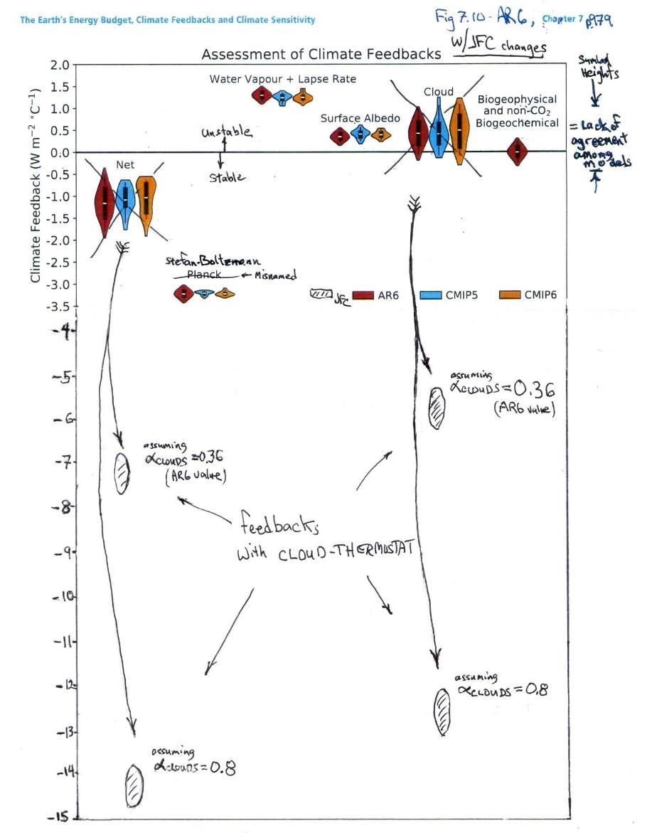
• AR6 (2021, Fig. 7.10, p. 979) estimates for the so-called feedback strengths (sensitivities) for various mechanisms.
• The AR6 Figure is corrected by replacing their estimate of λClouds , with the estimates calculated here for the cloud-feedback mechanism, under two scenarios - assuming cloud albedo = 0.36, and 0.8. In both scenarios, the cloud-feedback mechanism is dominant. [See Appendix D]
62
Part II - Conclusions
1. I have introduced here the cloud-thermostat mechanism. It is clearly the overwhelmingly dominant climate controlling feedback mechanism that controls stabilizes the Earth’s climate and temperature. It thereby prevents global warming and climate change.
2. The IPCC’s 2021 AR6 report (p.978) claims that climate stabilizing natural feedback mechanisms have a net (total) stabilizing strength of -1.16 ± 0.6 W/m2/K. My cloud feedback mechanism has a net stabilizing strength of anywhere between -5.7 to -12.7 W/m2/K, depending of one’s assumptions regarding the albedo of clouds.
3. My cloud thermostat mechanism provides nature’s own Solar Radiation Management System. This mechanism already exists. It is built in to nature’s own cloud factory. It works very well to stabilize the Earth’s temperature on a long term basis. And, it is free!
63
“Recommendations for policy makers - 1”
1. There is no climate crisis! There is, however, a very real problem with providing a decent standard of living to the world’s now enormous population. There is indeed an energy shortage crisis. The latter is being unnecessarily exacerbated by what, in my opinion, is incorrect climate science, and by government’s associated incorrect muddled response to it.
2. Government and business are currently needlessly spending trillions of dollars on efforts to limit the greenhouse gasses, CO2 and CH4, in the Earth’s atmosphere.
3. CO2 and CH4 are not pollutants. They must be removed from every list of defined pollutants. They have a negligible effect on the climate. Trillions of dollars can be saved by this one simple measure alone! Additionally, the CO2 Coalition points out that atmospheric CO2 is actually beneficial.
64
“Recommendations for policy makers - 2”
4. I recommend that all efforts to limit environmental carbon should be terminated immediately! Trillions of dollars can be saved by eliminating carbon caps, carbon credits, carbon sequestration, carbon footprints, zero-carbon targets, carbon taxes, anti-carbon policies and fossil-fuel limits, in energy policy and elsewhere.
5. Government requirements and subsidies for electric vehicles, all electric power, solar and wind power, etc. should all be eliminated.
6. Geoengineering programs to reduce global warming should be cancelled.
7. To paraphrase (and update for inflation) the late Sen. Everett Dirksen’s 1969 comment about the Vietnam war and Apollo programs, and redirect it to the IPCC’s anti-carbon policies“A trillion here, a trillion there, and pretty soon you’re talking real money.”
65
Appendix A. An energy-conservation Theorem phrased
in terms of albedos
Theorem: The albedo of a composite area is the area-weighted average of the individual component areas’ albedos -
α ALL-sky = fClouds X αClouds + fCLR-sky X αCLR-sky
Definitions:
OSRALL-sky ≡ Outgoing SW Radiation irradiance for the whole Earth.
OSRCLR-sky ≡ Outgoing SW Radiation irradiance in cloud-free areas of the Earth.
OSRClouds ≡ Outgoing SW Radiation irradiance in cloudy areas of the Earth.
TOAINC ≡ Incident SW Radiation irradiance for the whole Earth.
fClouds ≡ cloudy-area fraction of the Earth.
fCLR-sky ≡ cloud-free area fraction of the Earth.
αALL-sky ≡ OSRALL-sky / TOAINC = albedo (SW reflectivity) for the whole Earth.
αCLR-sky ≡ OSRCLR-sky / TOAINC = albedo for cloud-free areas of the Earth.
αClouds ≡ OSRClouds / TOAINC = albedo for cloudy areas of the Earth.
Assumtions:
Conservation of area: fClouds + fCLR-sky = 1. (1)
Conservation of energy, OSRALL-sky = OSRCLR-sky + OSRClouds. (2)
66
Proof:
Evaluate the above expressions, using Equations (1) and (2) for α ALL-sky, αClouds, and αCLR-sky , α ALL-sky = fClouds X αClouds + fCLR-sky X αCLR-sky, (3)
Corollary: α Clouds = α ALL-sky / fClouds – ((1/ fClouds) – 1) α CLR-sky (4)
This latter formula is useful for evaluating the cloudy-sky albedo when ALL-sky albedo, CLR-sky albedo, and cloud fraction are all known.
67
Appendix B. Application of the albedo conservation Theorem to data from the Fig. X.6 AR6 (2021 p.934) power-flow map data
The IPCC’s numbers from AR6 are shown here to require the silly number, αClouds = 0.36. (The notation used here is defined above in Appendix A.)
First note that the AR6 all-sky diagram implies that the all-sky albedo is
αALL-sky ≡ OSRALL-sky / TOAINC = 100 / 340 = 0.3.
The clear-sky diagram (lower power flow map), for fCLR-sky = 0.33 (i.e. for 33% of the Earth’s area), simultaneously implies that the clear-sky albedo is
αCLR-sky ≡ OSRCLR-sky / TOAINC = 53 / 340 = 0.16.
For the cloud fraction, fClouds = 0.67, the albedo conservation corollary (in Appendix A) shows that the cloudy sky albedo is αClouds = 0.36.
This value for αClouds seems conspicuously wrong by about a factor of two! If true, then clouds in the NASA satellite photos of Fig. X.7 should appear as barely brighter (more reflective of light) than the whole-Earth average. They don’t. For comparison, a sheet of white paper is about 99% reflective. Clouds in the photos appear visually a lot brighter than dessert-color brown or ocean-color blue, and appear much closer to paper-color white,.
Also, note that the commonly accepted value for nearly all types of clouds is about αClouds = 0.8 - 0.9. See, for example, the measurements and estimates by Griggs (1968), Cheylek et al. (1984), Wetherald and Manabe (1988), Stephens and Greenwald (1991). The measurements of αClouds for Pacific Ocean stratus clouds by Griggs (1968) were done from a DC3 aircraft, and, of course, do not include the added contribution from atmospheric (blue-sky) Rayleigh (back) scattering, that Top of Atmosphere albedos αClouds and αCLR-sky must both further add.
68
Appendix C. Feedback Analysis of climate systems [as
per Sherwood et al. (2020)]
• Sherwood et al. (2020) use the symbol ΔN, to represent the downward-flowing energy imbalance, calculated at the Top of Atmosphere. This is the quantity the I have discussed above that is used by the IPCC to define global warming. It is the primary target of the IPCC’s computer modelling and observational efforts.
• If the imbalance, ΔN, is negative, the earth is cooling. If it is positive, the Earth is warming.
• For any given feedback mechanism, Sherwood et al. (2020) calculate the overall feedback strength (sensitivity) as the derivative of ΔN with respect to the Earth’s surface temperature,
λ ≡ dΔN / dTSurface.
If λ is negative, the feedback stabilizes the system. If , if λ is positive, the system is unstable.
• If the system has a variety of independent mechanisms, and each mechanism, labeled j, relies on an associated intermediate variable, xj , then the total system’s feedback strength is calculated using the chain rule for derivatives, as per
j = Σj (∂ΔN /∂xj) X (∂xj/∂TSurface).
• For example, the primary temperature stabilizing feedback mechanism is via the Stefan-Boltzmann law’s σT4 dependence of far-infrared (LW) energy reemission by the Earth. Here, σ, is the Stephan-Boltzmann constant. Sherwood et al. (2020, p.19) calculate the (misnamed) feedback parameter, λPlanck, for StefanBoltzmann law negative feedback, as λPlanck = -3.3 W/m2/K.
(The Stefan-Boltzmann Law was discovered in 1879. Planck’s law was not discovered until 1900. The quantity called λPlanck should properly be called λStefan-Boltzmann.)
λ
Σ
λ
≡
j
69
Appendix D. Feedback strength of the cloud thermostat mechanism
• To calculate the feedback strength for the cloud thermostat, note that the shadowing of the oceans by clouds modulates the sunlight irradiance reaching the surface, SWdown. In doing so, it similarly modulates ΔN. A first step in the calculation is to use the albedo conservation theorem, and the terminology introduced in Appendix A, to evaluate SWdown , as per
SWdown ≡ (1-αALL-sky) TOAINC = [1–(fClouds αClouds + fCLR-sky αCLR-sky)] TOAINC, where TOAINC is the incident sunlight power.
• For some strange reason, Sherwood et al. (2020) arbitrarily structure the allowable forms for ΔN to prohibit the use of fClouds as an intermediate variable xClouds . I ignore this silly restriction here! [Cess (1976) did use use fClouds as an intermediate variable and obtained similar results to those presented here.]
• The climate feedback parameter for the specific cloud thermostat process is
λClouds ≡ d SWdown / dTsurface . It may be expanded using the chain rule, and fClouds as an intermediate variable, yielding
λClouds = d SWdown /dTsurface = (∂ SWdown /∂ fClouds) X (∂ SWdown /∂Tsurface) = – (fClouds αClouds) TOAINC (∂ fClouds /∂Tsurface).
• Finally one may reasonably estimate the remaining important factor, ∂fClouds/∂Tsurface . It is found by noting that both the precipitation rate of clouds and the evaporation rate are a sensitive functions of surface temperature. Both are directly proportional to the vapor pressure of seawater, whose temperature dependence is about 7-8% per degree Kelvin (or Celsius). i.e. ∂fClouds/∂Tsurface ≈ 0.07/K
70
