Issuu

Economics 21st Edition by McConnell

ISBN 1259723224

9781259723223

Download solution manual at: https://testbankpack.com/p/solution-manual-foreconomics-21st-edition-by-mcconnell-isbn1259723224-9781259723223/

Download full test bank at : https://testbankpack.com/p/test-bank-foreconomics-21st-edition-by-mcconnell-isbn1259723224-9781259723223/

Chapter 09 - Businesses and the Costs of Production

McConnell Brue Flynn 21e

DISCUSSION QUESTIONS

1. Distinguish between explicit and implicit costs, giving examples of each. What are some explicit and implicit costs of attending college? LO1

Answer: Explicit costs are payments the firm must make for inputs to non-owners of the firm to attract them away from other employment, for example, wages and salaries to its employees. Implicit costs are nonexpenditure costs that occur through the use of self-owned, self-employed resources, for example, the salary the owner of a firm forgoes by operating his or her own firm and not working for someone else. The explicit costs of going to college are the tuition costs, the cost of books, and the extra costs of living away from home (if applicable). The implicit costs are the income forgone and the hard grind of studying (if applicable).

2. Distinguish between accounting profit, economic profit, and normal profit. Does accounting profit or economic profit determine how entrepreneurs allocate resources between different business ventures? Explain. LO1

Answer: Accounting profit equals sales revenue minus explicit costs, such as material, the wages of employees, etc…

Normal profit equals the accounting profit you could have potentially earned in a different (or alternative) business venture. This gives us a true measure of the opportunity cost of the current business venture. Economists classify normal profits as costs, since in the long run the owner of a firm would close it down if a normal profit were not being

Chapter 09 - Businesses and the Costs of Production 9-1

earned. Since a normal profit is required to keep the entrepreneur operating the firm, a normal profit is a cost.

Economic profit equals the accounting profit minus the additional implicit costs of the business. This includes entrepreneurial ability, forgone interest, forgone labor income, etc...

Economic profit determines how entrepreneurs allocate resources between different business ventures. If economic profit is greater zero this implies the business venture is earning above average normal profits (more than other alternative business ventures on average), thus more resources will flow towards this activity. The opposite is true when economic profit is negative.

Chapter 09 - Businesses and the Costs of Production 9-2

3. Complete the table directly below by calculating marginal product and average product.

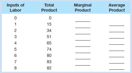
Plot the total, marginal, and average products and explain in detail the relationship between each pair of curves. Explain why marginal product first rises, then declines, and ultimately becomes negative. What bearing does the law of diminishing returns have on short-run costs? Be specific. “When marginal product is rising, marginal cost is falling. And when marginal product is diminishing, marginal cost is rising.” Illustrate and explain graphically. LO2

Chapter 09 - Businesses and the Costs of Production 9-3

Answer: Table: Inputs of labor Total product Marginal product Average product 0 1 2 3 4 5 6 7 8 0 15 34 51 65 74 80 83 82 NA 15 19 17 14 9 6 3 -1 NA 15 17 17 16.25 14.8 13.33 11.86 10.25

Plots, or graphs, for this problem will need to be done by students and instructors.

MP is the slope the rate of change of the TP curve. When TP is rising at an increasing rate, MP is positive and rising. When TP is rising at a diminishing rate, MP is positive but falling. When TP is falling, MP is negative and falling. AP rises when MP is above it; AP falls when MP is below it.

MP first rises because the fixed capital gets used more productively as added workers are employed. Each added worker contributes more to output than the previous worker because the firm is better able to use its fixed plant and equipment. As still more labor is added, the law of diminishing returns takes hold. Labor becomes so abundant relative to the fixed capital that congestion occurs and marginal product falls. At the extreme, the addition of labor so overcrowds the plant that the marginal product of still more labor is negative total output falls. Because labor is the only variable input and its price (its wage rate) is constant, MC is found by dividing the wage rate by MP. When MP is rising, MC is falling; when MP reaches its maximum, MC is at its minimum; when MP is falling, MC is rising.

4. Why can the distinction between fixed costs and variable costs be made in the short run?

Classify the following as fixed or variable costs: advertising expenditures, fuel, interest on company-issued bonds, shipping charges, payments for raw materials, real estate taxes, executive salaries, insurance premiums, wage payments, depreciation and obsolescence charges, sales taxes, and rental payments on leased office machinery. “There are no fixed costs in the long run; all costs are variable.” Explain. LO3

Answer: The distinction can be made because there are some costs that do not vary with total output. These are the fixed costs that, fundamentally, are related to the scale or size of the plant. In the short run, by definition, the scale of the plant cannot change: The firm cannot bring in more machinery or move to a larger building. All costs that are related to the scale ofthe plant coststhat continue to be incurredeven thoughthe firm’s output may be zero are fixed costs. On the other hand, the firm can increase its output by using its plant its fixed capital more intensively, that is, by hiring more labor, or by using more materials. But by doing so, it will increase its operating costs, its variable costs.

Advertising expenditures: variable costs (although it may be reasonable to argue a fixed component). Fuel: variable costs. Interest on company-issued bonds: fixed costs. Shipping charges: variable costs. Payments for raw materials: variable costs. Real estate taxes: fixed costs. Executive salaries: fixed costs. Insurance premiums: fixed costs. Wage payments: variablecosts. Depreciation and obsolescence charges: fixedcosts. Sales taxes: variable costs. Rental payments on leased office machinery: fixed costs (although it is possible that short-term lease arrangements on some types of office equipment may rise or fall with output).

In the long run, the firm can, by definition, get out of paying all of its short-run fixed costs; its lease is up, it can fire its executives without penalty, the insurance has run out, and so on. All of its costs at this moment, then, are variable. It can decide to continue producing at thesamescaleandthusreassumeallitspreviousfixedcostsforthenext short-runperiod; or it can decide to increase its scale and thus increase its fixed costs; or it can decide to go out of business and thus have no costs at all.

Chapter 09 - Businesses and the Costs of Production 9-4

5. List several fixed and variable costs associated with owning and operating an automobile. Suppose you are considering whether to drive your car or fly 1,000 miles to Florida for spring break. Which costs fixed, variable, or both would you take into account in making your decision? Would any implicit costs be relevant? Explain. LO3

Answer: Fixedcostsassociatedwithowningandoperatinganautomobileincludetheprice of the car (probably monthly payments); insurance; driver’s license; car license; and depreciation.

Variable costs associated with owning and operating an automobile include gasoline, oil, lubricants; repairs; car wash; and depreciation, which is also in part a variable cost since the more the car is driven, the more it depreciates.

The costsof drivingto FortLauderdale arethe same variable costs (including depreciation) listed above. Going by plane, the variable cost is the cost of the ticket. It would probably be cheaper to drive but this would leave out the relevant implicit cost my time and the wear and tear on myself of driving there and back. The plane would be faster. How much is it worth to me to arrive sooner and stay longer and be fresher on arrival? On the other hand, maybe I’d find the car useful around Fort Lauderdale, and having one’s own car saves the variable cost of renting if one flies.

6. Use the concepts of economies and diseconomies of scale to explain the shape of a firm’s long-run ATC curve. What is the concept of minimum efficient scale? What bearing can the shape of the long-run ATC curve have on the structure of an industry? LO4

Answer: The long-run ATC curve is U-shaped. At first, long-run ATC falls as the firm expands and realizes economies of scale from labor and managerial specialization and the use of more efficient capital. The long-run ATC curve later turns upward when the enlarged firm experiences diseconomies of scale, usually resulting from managerial inefficiencies.

The MES (minimum efficient scale) is the smallest level of output needed to attain all economies of scale and minimum long-run ATC.

If long-run ATC drops quickly to its minimum cost which then extends over a long range of output, the industry will likely be composed of both large and small firms. If long-run ATC descends slowly to its minimum cost over a long range of output, the industry will likely be composed of a few large firms. If long-run ATC drops quickly to its minimum point and then rises abruptly, the industry will likely be composed of many small firms.

Chapter 09 - Businesses and the Costs of Production 9-5

7. LAST WORD Does additive manufacturing rely on economies of scale to deliver low costs? What are two ways in which additive manufacturing lowers costs? Besides what's written in the book, might there be another reason to expect 3-D blueprints to be inexpensive? (Hint: Think in terms of supply and demand.)

Answer: No, additive manufacturing does not rely on mass production and mass sales to lower its costs. Additive manufacturing will eliminate the large fixed costs attributed to building factories, as well as eliminating transportation costs required to ship resources and finished goods.

Once 3-D printers become widespread, the business to be in will be designing 3-D blueprints. Due to many new companies making these blueprints, the supply of them will increase. This increase in supply will drive the price down.

REVIEW QUESTIONS

1. Linda sells 100 bottles of homemade ketchup for $10 each. The cost of the ingredients and the bottles and the labels was $700. In addition, it took her 20 hours to make the ketchup and to do so she took time off from a job that paid her $20 per hour. Linda’s accounting profit is _____________ while her economic profit is ______________. LO1

a. $700; $400

b. $300; $100

c. $300; negative $100

d. $1,000; negative $1,100

Answer: e; $300; negative $100.

Linda’s revenue is $1,000 (=100 bottles of ketchup sold at $10 each). Linda’s explicit costs for ingredients, bottles, and labels are $700. Thus her accounting profit (which subtracts explicit costs from revenue) is $300 (=$1,000 of revenue minus $700 of explicit costs).

Linda’s implicit cost is the opportunity cost of the 20 hours of labor that she put into making the ketchup. Because she gave up making $20 per hour for each of those 20 hours of labor, the implicit cost of her labor is $400 (=$20 per hour times 20 hours). Thus her economic profit (which subtracts both explicit costs and implicit costs from revenue) is negative $100 (=$1,000 in revenue minus $700 in explicit costs minus $400 in implicit costs).

2. Which of the following are short-run and which are long-run adjustments? LO1

a. Wendy’s builds a new restaurant.

b. Harley-Davidson Corporation hires 200 more production workers.

c. A farmer increases the amount of fertilizer used on his corn crop.

d. An Alcoa aluminum plant adds a third shift of workers.

Chapter 09 - Businesses and the Costs of Production 9-6

Answer:

a. Long-Run. This is a capital investment, which takes time to become productive.

b. Short-Run. The new laborers can work immediately.

c. Short-Run. Although this takes time via the growing process, this is still a short-run adjustment. It influences the growth of current crops immediately.

d. Short-Run. The new laborers can work immediately.

3. A firm has fixed costs of $60 and variable costs as indicated in the table at the bottom of this page. Complete the table and check your calculations by referring to problem 4 at the end of Chapter 10. LO3

a.Graph total fixed cost, total variable cost, and total cost. Explain how the law of diminishing returns influences the shapes of the variable-cost and total-cost curves.

b.Graph AFC, AVC, ATC, and MC. Explain the derivation and shape of each of these four curves and their relationships to one another. Specifically, explain in nontechnical terms why the MC curve intersects both the AVC and the ATC curves at their minimum points.

c.Explain how the location of each curve graphed in question 3b would be altered if (1) total fixed cost had been $100 rather than $60 and (2) total variable cost had been $10 less at each level of output.

Chapter 09 - Businesses and the Costs of Production 9-7

a. See the graph below. Over the 0 to 4 range of output, the TVC and TC curves slope upward at a decreasing rate because of increasing marginal returns. The slopes of the curves then increase at an increasing rate as diminishing marginal returns occur.

b. See the graph below. AFC (= TFC/Q) falls continuously since a fixed amount of capital cost is spread over more units of output. The MC (= change in TC/change in Q), AVC (= TVC/Q), and ATC (= TC/Q) curves are U-shaped, reflecting the influence of first increasing and then diminishing returns. The ATC curve sums AFC and AVC vertically. The ATC curve falls when the MC curve is below it; the ATC curve rises when the MC curve is above it. This means the MC curve must intersect the ATC curve at its lowest point. The same logic holds for the minimum point of the AVC curve.

Table: Total product Total fixed cost Total variable cost Total cost Average fixed cost Average variable cost Average total cost Marginal cost 0 1 2 3 4 5 6 7 8 9 10 $60 60 60 60 60 60 60 60 60 60 60 $ 0 45 85 120 150 185 225 270 325 390 465 $0 105 145 180 210 245 285 330 385 450 525 $60 30 20 15 12 10 8.57 7.5 6.67 6 $45 42.5 40 37.5 37 37.5 38.57 40.63 43.33 46.5 $105 72.5 60 52.5 49 47.5 47.14 48.13 50 52.5 $45 40 35 30 35 40 45 55 65 75

2018

Answer:

c. (1) If TFC has been $100 instead of $60, the AFC and ATC curves would be higher by an amount equal to $40 divided by the specific output. Example: at 4 units, AVC = $25.00 [= ($60 + $40)/4]; and ATC = $62.50 [= ($210 + $40)/4]. The AVC and MC curves are not affected by changes in fixed costs.

(2) If TVC has been $10 less at each output, MC would be $10 lower for the first unit of output but remain the same for the remaining output. The AVC and ATC curves would also be lower by an amount equal to $10 divided by the specific output. Example: at 4 units of output, AVC = $35.00 [= $150 - $10)/4], ATC = $50 [= ($210 - $10)/4]. The AFC curve would not be affected by the change in variable costs.

4. Indicate how each of the following would shift the (1) marginal-cost curve, (2) averagevariable-cost curve, (3) average-fixed-cost curve, and (4) average-total-cost curve of a manufacturing firm. In each case specify the direction of the shift. LO3

a.A reduction in business property taxes.

b.An increase in the nominal wages of production workers.

c.A decrease in the price of electricity.

d.An increase in insurance rates on plant and equipment.

e.An increase in transportation costs.

Answer:

a. This is a change in the fixed cost. This implies there will be no change in MC or AVC. Since this is a decrease in fixed cost AFC shifts down and ATC shifts down (sum of AVC and AFC).

b. This is a change in variable cost. Since wages are now higher, MC shifts up, AVC shifts up, and ATC shifts up. There is no change in AFC.

c. This is a change in variable cost. The lower price of electricity implies MC shifts down, AVC shifts down, and ATC shifts down. There is no change in AFC.

d. This is a change in the fixed cost. This implies there will be no change in MC or AVC. Since this is an increase in fixed cost AFC shifts up and ATC shifts up.

e. This is a change in variable cost. Since transportation costs are now higher, MC shifts up, AVC shifts up, and ATC shifts up. There is no change in AFC.

Chapter 09 - Businesses and the Costs of Production 9-9

the

prior written consent of McGraw-Hill Education.

5. True or false. The U shape of the long-run ATC curve is the result of diminishing returns. LO4

Answer: false

The long-run ATC curve's U shape cannot be explained by diminishing returns. That is because the definitions of short run and long run that are used in microeconomics imply that diminishing returns can only take place in the short run.

To see why, recall that the short run is a period of time that is too brief for a firm to alter its plant capacity while the long run is a period long enough for a firm to adjust the quantities of all the resources that it employs, including plant capacity. The difference between those definitions matters because diminishing returns applies only when one productive resources or input is held constant. Thus, it cannot happen in the long run when, by definition, firms have had enough time to adjust all their inputs, including plant capacity.

So what does cause the U shape of the long-run ATC curve? The answer is economics and diseconomies of scale related to factors such as labor specialization and capital efficiency.

6. Suppose a firm has only three possible plant-size options, represented by the ATC curves shown in the accompanying figure. What plant size will the firm choose in producing (a) 50, (b) 130, (c) 160, and (d) 250 units of output? Draw the firm’s long-run average-cost curve on the diagram and describe this curve. LO4

Chapter 09 - Businesses and the Costs of Production 9-10

Answer:

(a) To produce 50 units, the firm will choose plant size #1, since its ATC is lower for this size firm in producing less than 80 units.

(b) To produce 130 units, the firm will choose plant size #2, since its ATC is lower for size #2 in producing between 80 and 240 units.

(c) To produce 160 units, the firm will choose plant size #2, since its ATC is lowest for producing between 80 and 240 units.

(d) To produce 250 units, the firm will choose plant size #3, since its ATC is lowest for production of more than 240 units.

The firm's long run average total cost curve will be the lower sections of the different plant size ATC schedules. Specifically, to the left of 80 units ATC1 will be the first section of the long run ATC. Between 80 and 240 ATC2 will make up the second section of the long run ATC. Finally, to the right of 240 ATC3 will make up the rest of the firm's long run ATC.

PROBLEMS

1. Gomez runs a small pottery firm. He hires one helper at $12,000 per year, pays annual rent of $5,000 for his shop, and spends $20,000 per year on materials. He has $40,000 of his own funds invested in equipment (pottery wheels, kilns, and so forth) that could earn him $4,000 per year if alternatively invested. He has been offered $15,000 per year to work as a potter for a competitor. He estimates his entrepreneurial talents are worth $3,000 per year. Total annual revenue from pottery sales is $72,000. Calculate the accounting profit and the economic profit for Gomez’s pottery firm. LO1

Answer: Accounting profit = $35,000; Economic profit = $13,000. Explicit costs are the direct costs incurred from production: $37,000 (= $12,000 for the helper + $5,000 of rent + $20,000 of materials). Implicit costs are the costs that are indirectly incurred by the activity: $22,000 (= $4,000 of forgone interest + $15,000 of forgone salary + $3,000 of entrepreneurship).

Accounting profit = $35,000 (= $72,000 of revenue - $37,000 of explicit costs); Economic profit = $13,000 (= $72,000 - $37,000 of explicit costs - $22,000 of implicit costs).

2. Imagine you have some workers and some hand-held computers that you can use to take inventory at a warehouse. There are diminishing returns to taking inventory. If one worker uses one computer, he can inventory 100 items per hour. Two workers can together inventory 150 items per hour. Three workers can together inventory 160 items per hour. And four or more workers can together inventory fewer than 160 items per hour. Computers cost $100 each and you must pay each worker $25 per hour. If you assign one worker per computer, what is the cost of inventorying a single item? What if you assign two workers per computer? Three? How many workers per computer should you assign if you wish to minimize the cost of inventorying a single item? LO2

Chapter 09 - Businesses and the Costs of Production

9-11

Answer: 1.25; 1.00; 1.09; 2

If you assign one worker per computer, the cost of inventorying a single item is $1.25. You incur the cost of the computer, $100, and the cost of employing one worker, $25, which is divided by the number of units inventoried, 100 (= ($100 + $25) / 100)).

If you assign two workers per computer, the cost of inventorying a single item is $1.00. You incur the cost of the computer, $100, and the cost of employing two workers, $50 ($25 each), which is divided by the number of units inventoried by the two workers, 150 (= ($100 + $50) / 150)).

If you assign three workers per computer, the cost of inventorying a single item is $1.09. You incur the cost of the computer, $100, and the cost of employing three workers, $75 ($25 each), which is divided by the number of units inventoried by the three workers, 160 (= ($100 + $75) / 160)).

To minimize the cost of inventorying a single item, you should assign two workers to each computer. This is the lowest cost per unit inventoried given the information above.

3. You are a newspaper publisher. You are in the middle of a one-year rental contract for your factory that requires you to pay $500,000 per month, and you have contractual labor obligations of $1 million per month that you can’t get out of. You also have a marginal printing cost of $0.25 per paper as well as a marginal delivery cost of $0.10 per paper. If sales fall by 20 percent from 1 million papers per month to 800,000 papers per month, what happens to the AFC per paper, the MC per paper, and the minimum amount that you must charge to break even on these costs? LO3

Answers:

AFC per paper rises from $1.50 per paper to $1.88 per paper; MC does not change; and the minimum amount that the paper must charge to break even rises from $1.85 per paper (= $1.5 million in fixed costs divided by 1 million papers plus $0.35 per paper in marginal costs) to $2.23 per paper (= $1.5 million in fixed costs divided by 800,000 papers plus $0.35 per paper in marginal costs).

Here Marginal Cost (MC) is constant, which implies that Average Variable Cost (AVC) is constant and equals MC. This does not imply Average Total Cost (ATC) is constant or has to equal MC. Total Cost (TC) = Fixed Cost (FC) + Variable Cost (VC)

Divide through by the quantity Q, which implies TC/Q = FC/Q + VC/Q. This gives us ATC = AFC + AVC.

Now, since MC is constant (each unit of output costs MC to produce), thus we have MCxQ = Variable Cost (VC). Note this is variable cost (VC) because we do not have to produce.

Divide this by Q, which implies that MC = VC/Q = AVC

Substituting this result into the ATC equation, we have ATC = AFC + MC (or AVC). Thus, MC and AVC are the same in this set-up.

The original average fixed cost (AFC) was $1.50, which equals the total fixed cost $1.5 million divided by the number of papers sold (1 million, the original amount). Note here that labor is treated as a fixed cost because of the contractual obligation (you must pay even if production stops, assuming the company does not file for bankruptcy) (=$1,500,000/1,000,000).

Chapter 09 - Businesses and the Costs of Production 9-12

Now assuming sales fall by 20% to 800,000 papers sold, the new average fixed cost (AFC) is $1.88. This equals the total fixed cost $1.5 million divided by the new number of papers sold, 800,000 (=$1,500.000/800,000). Thus, the AFC increases from $1.50 to $1.88 after the decrease in sales. The marginal printing and marginal delivery costs are still the same; therefore, marginal costs do not change.

To break-even before the decline in sales, the company needed to charge enough to cover the AFC, $1.50, and the average variable cost (AVC) of $0.35 (This is the sum of the printing cost and delivery cost per paper). Thus, the company needed to charge $1.85 per paper.

To break-even after the decline in sales, the company needs to charge enough to cover the AFC, $1.88, and the average variable cost (AVC) of $0.35 (This is the sum of the printing cost and delivery cost per paper, note this does not change because the cost is per paper). Thus, the company needed to charge $2.23 per paper.

4. There are economies of scale in ranching, especially with regard to fencing land. Suppose that barbed-wire fencing costs $10,000 per mile to set up. How much would it cost to fence a single property whose area is one square mile if that property also happens to be perfectly square, with sides that are each one-mile long? How much would it cost to fence exactly four such properties, which together would contain four square miles of area? Now, consider how much it would cost to fence in four square miles of ranch land if, instead, it comes as a single large square that is twomiles long on each side. Which is more costly fencing in the four, one-square-mile properties or the single four-square-mile property? LO4

Answers: $40,000 for the single one-square-mile property; $160,000 for four of the one-square-mile properties; $80,000 for the single four-square-mile property that is two-miles on each side; it is cheaper to fence in a single four-square-mile property than four, one-square mile properties.

Feedback: Consider the following example: Barbed-wire fencing costs $10,000 per mile to set up. How much would it cost to fence a single property whose area is one square mile if that property also happens to be perfectly square, with sides that are each one-mile long?

The answer is 4 times $10,000 for each side of the fence, or $40,000. How much would it cost to fence exactly four such properties, which together would contain four square miles of area? The four squares below represent our 4 properties. Each of these cost $40,000 to fence. Thus, the cost of fencing these four properties equals $160,000 (= 4 x $40,000).

Chapter 09 - Businesses and the Costs of Production 9-13

Now, consider how much it would cost to fence in four square miles of ranch land if, instead, it comes as a single large square that is two-miles long on each side. Here, we only need to fence the outside perimeter in the diagram below. First, recognize that each side of the square below is twice as long as the problem above (separate properties), which implies it is going to cost $20,000 to fence each side (2 miles long). There are four sides, so the total cost of fencing this area is $80,000 (= 4 x $20,000).

This implies that it is cheaper to fence a property of four square miles than four properties of one square mile. The cost savings comes from the fact that we do not need to fence off the inner sides of the square miles (dashed lines).

Chapter 09 - Businesses and the Costs of Production 9-14