
Active planar phased array, array factor (AF), particle swarm optimization (PSO), radar, transmit receive module (TRM)
ABSTRACT
With rapid development and advancement in the technologies, the trend of incorporating an „active‟ phased array configuration in majority of wireless, mobile, space and radar communication system is increasing day by day [1, 2]. Studies revealed that an active phased array configuration offers the collective advantages of high reliability, improved efficiency, low loss and higher sensitivity over a passive configuration [3]. An active phased array system contains several antenna elements assembled with individual solid state transmit receive module (TRM) to meet the required power aperture product. The system uses the abilities of active array to electronically steer the array beam instantaneously in any direction by controlling in build phase shifters of TRMs [4].
International Journal of Antennas (JANT) Vol.2, No.3, July 2016 DOI: 10.5121/jant.2016.2301 1
Samaresh
KEYWORDS
Evolutionary algorithms (EAs) have the potential to handle complex, multi dimensional optimization problems in the field of phased array. Out of different EAs, particle swarm optimization (PSO) is a popular choice. In a phased array, antenna element failure is a common phenomenon and this leads to degradation of the array factor (AF) pattern, primarily in terms of increased side lobe levels (SLLs), displacement of nulls and reduction in the null depths. The recovery of a degraded pattern using a cost and time effective approach is on demand. In this context, an attempt made to obtain an optimized AF pattern after fault in a 49 elements quasi circular aperture equilateral triangular grid active planar phased array using PSO. In the paper, multiple cases on recovery are discussed having a maximum 20% element failure. Each recovery is also further evaluated by different statistical analyses A dedicated software tool was developed to carry out the work presented in this paper.
ARRAY FACTOR OPTIMIZATION OF AN ACTIVE PLANAR PHASED ARRAY USING EVOLUTIONARY ALGORITHM
Bhattacharjee, Ashish Kumar, Manish Naja
Aryabhatta Research Institute of observational sciencES (ARIES), Nainital 263001, Uttarakhand, India
1.INTRODUCTION
Failure of single or multiple TRMs in such systems is a common occurrence which makes an antenna element become non radiative. In the event of the failure, the far field array factor (AF) pattern of the system degrades seriously in terms of increased side lobe levels (SLLs), displacement of nulls and reduction in the null depths. To get rid of such degradations, repair/ replacement of the faulty modules could be best choice, as it always gives the best recovery of the original AF pattern. However, such repair/ replacement in a space based or ground based systems commissioned with hundreds of TRMs will be expensive in terms of time and budget. Under such circumstances, without undergoing any repair/ replacement, evolutionary algorithms (EAs) could
be used as an alternative to recover the optimized pattern closest to the original by perturbing the input amplitudes and/ or phases of input excitations of remaining functional TRMs
This paper presents multiple cases on the recovery of the AF pattern of a 49 elements active planar phased array operating in very high frequency (VHF) band. Active array in VHF band has wide application in the areas of wind profiling and weather radar [20]. In the presented cases, the number of non working elements is increased to a maximum 20% of the total elements. The recovered pattern in each case is evaluated numerically by comparing the levels of first side lobes (FSLs) and the depth of the first nulls (FNs) with the corresponding values in the original AF pattern.
MN jmTTnTTxxsyys mn mn AFAe
00
International Journal of Antennas (JANT) Vol.2, No.3, July 2016
EAs are inspired by the biological models of evolution and natural selection [5, 6]. To solve a particular problem using EAs, a situation is created in which potential solutions can evolve. The situation is outlined by the parameters of the problem that pushes the algorithm towards optimal solutions. Most commonly used EAs are genetic algorithm (GA) [7], particle swarm optimization (PSO) [8, 9], cuckoo search (CS) [10], and artificial bee colony (ABC) [11]. Several studies have been reported on optimization of AF pattern by amplitude and/ or phase perturbation using EAs for linear array [12 15]. The present work deals with recovery of the AF pattern of an active planar phased array by recalculating a new set of amplitudes of input excitations of working elements using PSO. Being a stochastic technique and based on the movement and intelligence of swarms, PSO has gained an immense popularity in the field of electromagnetics [16]. The reason behind selecting PSO is that PSO algorithm has the advantages of its simplicity and less computational complexity over the other EAs. The computational time taken by PSO to arrive at the desired solution is also less as compared to other EAs [17 19].
2.ARRAY CONCEPT
where, dx and dy = inter element spacing along X and Y direction respectively; Tx = (2π/λ) dx cos(αx); Ty = (2π/λ) dy cos(αy); Txs = (2π/λ) dx cos(αxs ) ; Tys = (2π/λ) dy cos(αys); cos(αx) = sin(θ)cos(φ); cos(αy) = sin(θ) sin(φ); cos(αxs) = sin(θo)cos(φo); cos(αys) = sin(θo) sin(φo); and Amn = Amplitude of input excitation of the mn th element.
2
Fig. 1. A planar phased array
The AF pattern of an active planar phased array consisting of M x N identical elements placed on XY plane (Fig. 1) scanning to a direction (θo, φo) may be expressed as [4]: 11 [()()](,) (1)

where, EP(θ,φ) is the Element Pattern (EP) of an antenna element at (θ,φ) plane.
The phasing of mn th element, ψmn for beam steering is calculated as mTxs + nTys and the far field radiation pattern of the array is: ff(θ,φ) = AF(θ,φ) x EP(θ,φ) (2)
The choice of different parameters and the constants in above two equations can be decided according to the work described in [22 25]. During the process of algorithm, the Pbest and Gbest are decided according to the criteria set by a fitness function (FF) [16]. A FF plays a vital role in controlling the performance of the algorithm. The selection of FF depends on the type and complexities present in the identified problem.
where, vn+1 and vn are the velocity vectors of the particle in the present and previous iterations respectively; Xn is the current position of the particle; w is the inertial weight which varies as the algorithm progresses and determines the weight by which the particles current velocity depends on its previous velocity; c1 is the cognitive coefficient controlling the pull to the Pbest position; c2 is the social rate coefficient controlling the pull to the Gbest position; rand1 and rand2 are the random numbers uniformly distributed in (0, 1); Δt is the time difference between the two successive positions of the particles and is most often taken as unity. The next position, Xn+1 of particle in the search space is calculated as:
4.METHODOLOGY OF THE WORK
International Journal of Antennas (JANT) Vol.2, No.3, July 2016
3.PSO
The PSO is a population based search strategy which is applied in an N dimensional search space containing set of points, referred as particles. These set of particles moves in the search space with velocities that are dynamically adjusted according to their historical performance as well as the experience and knowledge of its neighbours. During movement, at each iteration, the particles update their velocities according to the best positions already found by themselves as personnel best (Pbest) and global best (Gbest) [16].
1122 ,, 1 ()() ... best nnbest nn nninertia cognitivepersonalcomponentsocialneighbourhoodcomponent PXGX vwvcrandcrand tt (3)
3
11nnn XXvt (4)
EAs are stochastic optimization techniques popularly being used for real life problem solving tasks in wide and diverse range of application areas like science, engineering, medical and economics [5, 6] and [21]. Among all EAs inspired from biological process, the PSO technique is simple, effective and capable of handling tricky multidimensional nonlinear optimization problems across the fields [16 19]. The PSO was originally introduced in 1995 by Russell Eberhart, an electrical engineer, and James Kennedy, a social psychologist [8, 9]. Here it is necessary to mention that the present work is not intended to carry an extensive review on PSO, and therefore only the main steps of the algorithm are discussed.
After finalizing the structure of the test array, a suitable FF is developed and expressed as equation (5). There could be many possibilities of the FF depending on the factors decided to achieve the optimization. The present FF is developed after a number of trials to bring the solution close to the optima by minimizing it till last iteration. The weights (a1, a2, a3 and a4) in the FF equation are taken as unity.
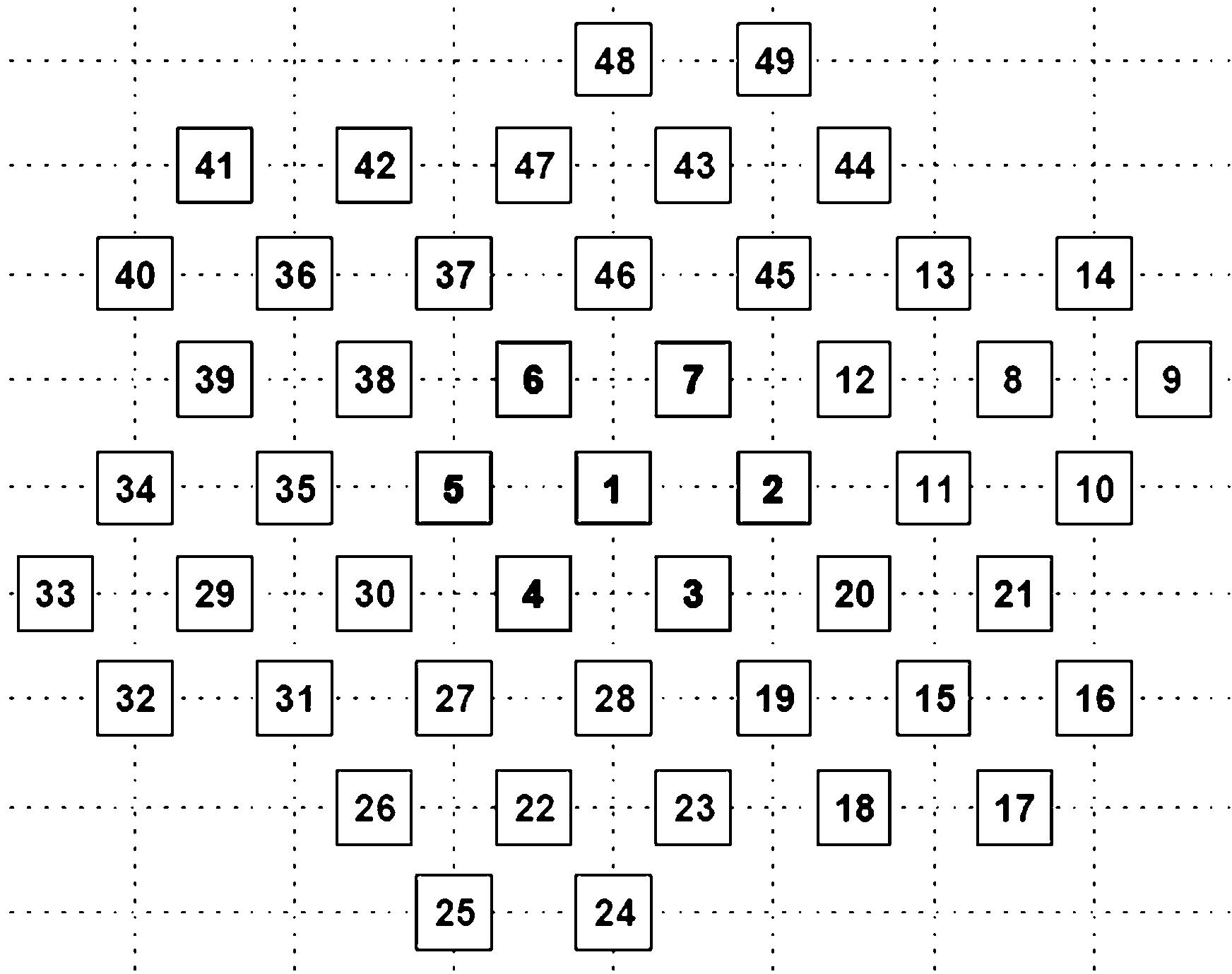
In the present work, a planar phased array having a quasi circular aperture is considered as the test array. The diagram of the array shown in Fig. 2 is populated with 49 elements, each represented by a square box labeled with a fixed numerical number for easy identification of element location. Elements of the array are arranged as equilateral triangular grid in 9 rows and 15 columns. During the design of the array geometry, it is attempted to make the periphery of the aperture close to circular to maintain angular symmetry in the AF pattern. A configuration of a planar array having circular or near to circular aperture with triangular grid gives a grating lobe free AF pattern at maximum possible off zenith angle with comparatively low FSLs without any amplitude tapering. Triangular grid also helps to reduce the number of elements demanded to fill a certain aperture [26]. These inherent advantages make the configuration a popular choice in applications like wireless, space borne synthetic aperture radar (SAR), weather radar, wind profilers [20], [27 29]
4
International Journal of Antennas (JANT) Vol.2, No.3, July 2016
Balanis says that the characteristic of an AF pattern can be broadly determined by the three levels: main beam, FSLs and FNs [30]. F1, F2 and F3 of FF uses these three levels of optimized and original patterns for deciding movement of particles in problem space. To test the
Fig. 2. The test array
11223344 FFaFaFaFaF (5) where, 2 1 [(0,0)(0,0)] psooriginalFAFAF 2 2__[] FSLpsoFSLoriginalFAFAF 2 3__[] FNpsoFNorigFAFAF 90 2 4 90 [(,)(,)] psooriginal FAF0AF0
EP of the array elements is considered as isotropic and initial amplitude of input excitations are taken as unity. The inter element spacing is kept 0.7 λ which places the rows and columns at 0.88 m and 1.02 m apart, respectively. Regardless of aperture or grid structure, the AF equation described in equation (1) takes individual element location as inputs. The same equation is used for calculating the AF of the test array. Effect of mutual coupling among elements is not considered during the analysis and discussion.
5
Different schemes on variation of „w‟ of equation (3) are tested, and finally for faster convergence „ w‟ is linearly decreased over 100 iterations from 0.9 to 0.4. The same tool can be used for optimization of any configurations of planar phased array by modifying the elements co
effectiveness of the PSO algorithm for the present problem with the FF, a software tool is developed. The coding of the tool is done based on the array concepts and the PSO algorithm. The tool takes the values of all the PSO parameters and the location of non working element as user inputs. Research revealed that PSO can achieve faster convergence towards optima with less oscillation by careful selection of its parameters [22 25]. After a detailed study, following values of the PSO parameters are fed into the developed tool and kept fixed in all the presented
Amn of equation (1) is written as (1+ μmn), where, μmn is introduced to represent the perturbation required in initial amplitude of the input excitations of working elements for recovery. Each iteration produces a new set of μmn which is algebraically added with unity to generate a new set of amplitudes for calculating the AF in present iteration required by all four entities of FF. The perturbations are restricted within a window of ±0.3, so the final amplitude factor, Amn is restricted within a boundary between 0.7 and 1.3, which is equal to ± 30% perturbation of initial amplitude. The window in amplitude factor can be linked with the tuning of power amplifier modules in TRMs. In practical application, depending on the type and quality of a power amplifier module, the set window may vary. Based on the methodologies, the results obtained after single run for each case are presented and discussed in the next section.
Fig. 3. Original AF pattern of the test array
International Journal of Antennas (JANT) Vol.2, No.3, July 2016
of particles = 200, No of iterations =100, Cognitive component (c1) = 2, and Social component (c2) =1
5.RESULTS AND DISCUSSION
The original AF pattern of the test array in normalized form without any element failure at zenith (θo, = 0 , φo = 0 ) is depicted in Fig. 3. From the figure, it is noted that the levels of FSLs are 19.08 dB down whereas the depths of FNs are 38.84 dB down from the peak level of the main beam which is at 0 dB after normalization. Throughout the work, the recovery of the pattern at zenith is only presented. No beam steering to other elevation (θo) or azimuth (φo) plane is introduced during the pattern optimization. After recovery in each case, the original AF, AF with fault and PSO optimized AF patterns are presented in a single figure for visual comparison and performance evaluation.

Inordinates.thecode,
cases.No
Fig. 4. AF patterns for case 1
Case 2: Work advances with three elements failure at locations 5, 2 and 28 selected randomly as user inputs. With these three non working elements, the levels of FSLs increase to 16.52 dB. But in opposite of the case 1, the depths of FNs increase to 49.67 dB with one degree shift towards the main beam. Again the tool runs to recover the original pattern by amplitude perturbation of remaining 46 working elements. Both fault and PSO optimized patterns with original one are depicted in Fig. 5.


Fig. 5. AF pattern for case 2
International Journal of Antennas (JANT) Vol.2, No.3, July 2016
6
In the next couple of paragraphs detailed evaluations on the AF pattern recovery in four different cases using the developed methodologies are discussed. Work starts with the recovery of the original pattern when a single element is made non working. Thereafter, number of non working elements are increased in subsequent cases to three, five and ten, respectively. The locations of the non working elements are picked up randomly.
Case 1: In the first case the center element at location 1 is made non working. The presence of a non working element at the said location increases the levels of both FSLs and FNs by 1.64 dB and 7.16 dB, respectively. After creation of the fault, now the tool runs with set PSO parameters to recover the original pattern. At the end of 100th iteration with 200 particles, the tool produces an optimized AF pattern close to the original one shown in Fig. 4. The tool has recovered the pattern by generating a new set of amplitudes of input excitations of 48 working elements and brings down the levels of FSLs and FNs to 19.09 dB and 38.87 dB, respectively resulting very close matching with the corresponding values in the original pattern.
7
The figure illustrates that the optimized pattern nicely follows the original pattern at every location of θ with hardly any variation in the levels. The shifting of FNs after faults is also rectified by placing them exactly at their original locations.

Case 3: Till now the tool has shown satisfactory performances in recovering the optimized pattern closest to the original after the occurrence of faults. But to imitate a more complex situation in an active phased array having hundreds of TRM, the tool is tested further with 10% non working elements i.e. 5 of 49 elements. The location numbers of non working elements are randomly taken as 37, 12, 30, 1 and 18. Remaining 44 working elements with a void at said locations produces a pattern with phenomena entirely opposite to the occurrences in the last two cases. FSLs of the fault pattern remain at very close to its original levels with one degree shift towards the main beam, whereas the second side lobes (SSLs) increase from 20.87 dB to 15.9 dB. These increased SSLs may pick up a strong interference signal from any external source and may raise the probability of occurrence of ambiguous detection [4] and [30]. Fig. 6 plots the AF pattern with faults at the said locations. The plot also depicts that the optimized pattern achieved after the final iteration is made highly resemble the original pattern. After optimization, the maximum levels of SLLs are brought down to 20.84 dB close to the original value 20.87 dB. In optimized pattern, the shifts in FSLs are rectified and original levels are also maintained.
Fig. 6. AF pattern for case 3
Case 4: To add much more complexity, the number of non working elements is increased further to ten which is equal to 20 % of the total elements. The position numbers of the fault elements are again randomly selected as 49, 42, 13, 5, 10, 32, 31, 19, 26 and 17. Fig. 7 presents the AF pattern before and after faults. The fault pattern is deformed to a typical formation. The lobes after second nulls are merged together and pop up to maximum 15.98 dB at ±30o. This merging eliminates the third and fourth nulls in both sides of the main beam. In opposite, on occurrence of merging, FSLs shift downward by approximately 10 dB. This downward shifting of FSLs could be better at the cost of the deformation, but the popping up of second and third side lobes could damage the entire application by inviting strong interferences into the system.
International Journal of Antennas (JANT) Vol.2, No.3, July 2016
Fig. 7. AF pattern for case 4
Thevalues.convergence
profiles of 200 particles obtained by minimizing the FF are presented in Fig. 8.

Once again the tool runs in the quest of searching a new set of amplitudes for the remaining 39 working elements for correcting the failed pattern. The optimized pattern after recovery is presented in Fig. 7. The pattern illustrates that the process of recovery is successfully handled by the tool to a great extent. FSLs are pulled up to the values of the original pattern. The region after FSL in both sides of the main lobe is restructured at every point and brought near to the original
The figure illustrates that the profiles of convergence are nicely damped and reached closest to optima at around 70th iteration. Out of 200 particles, the 81th particle emerges as the global best to produce the best optimized AF pattern.

Fig. 8. Convergence profiles of the FF for case 4
The final amplitudes of input excitations of 39 working elements of case 4 are displayed in Fig. 9. The values of excitations are represented by a grey scale whose values vary between 0.6 and 1.3. The figure depicts the final excitations searched by the tool within the set window. In the figure, the non working elements are represented by only number without any shaded box.
International Journal of Antennas (JANT) Vol.2, No.3, July 2016 8
A comparative summary on the values of the critical parameters of AF patterns in original, fault and recovered conditions discussed in above four cases is presented in Table 1.
International Journal of Antennas (JANT) Vol.2, No.3, July 2016
Case 2 FSLs 19.08 dB 16.52 dB 19.08 dB
FNs 38.84 dB 49.67 dB 38.85 dB FNBW 28o 26 o 28 o
The degree of recovery of each case is further examined and compared using linear correlation coefficient (LCC), median absolute deviation correlation coefficient (MADCC), linear least square regression (LLSR) and root mean square error (RMSE) statistical methods [31]. The results after examination are tabulated in Table 2.

Case 1 FSLs 19.08 dB 17.44 dB 19.09 dB FNs 38.84 dB 31.68 dB 38.87 dB
Fig. 9. Final amplitude distribution for case 4
Case 3 FNBWFNsFSLs 19.08 dB 38.84 dB 28o 18.28 dB 39.48 dB 26 o 19.15 dB 38.16 dB 28 o
FNBW 28o 26 o 28 o
Case 4 FSLs 19.08 dB 27.73 dB 19.18 dB FNs 38.84 dB 32.65 dB 36.87 dB FNBW 28o 30 o 28 o
9
Table-1. Comparative results
Cases Parameters Original After fault recoveryAfter
[7] J. F. Frenzel, "Genetic algorithms," Potentials, IEEE, vol.12, no.3, pp.21 24, Oct. 1993.
Case 1 0.9965 0.9999 0.8564 0.9991 0.9931 0.9999 1.9029 0.0395
[2] J. Ronghong, Y. Sheng, L. Xianling, and G. Junping, "Research on planar antenna arrays," Antenna Technology: "Small Antennas, Novel EM Structures and Materials, and Applications" (iWAT), International Workshop on, pp.140 142, 4 6 Mar. 2014
Case 4 0.9883 0.9992 0.7615 0.9643 0.9768 0.9985 4.1567 1.0870
10
REFERENCES
International Journal of Antennas (JANT) Vol.2, No.3, July 2016
[5] T. Bäck and H. P. Schwefel, “An overview of evolutionary algorithms for parameter optimization,” Evol. Comput., vol.1, no.1, pp. 1 24, Spring 1993.
[6] K. R. Krishnanand, S. K. Nayak, K. B. Panigrahi, and P. K. Rout, "Comparative study of five bio inspired evolutionary optimization techniques," Nature & Biologically Inspired Computing, NaBIC, World Congress on, pp. 1231 1236, 9 11 Dec. 2009.
Case 3 0.9821 0.9997 0.0683 0.9679 0.9646 0.9995 4.2718 0.4674
Cases LCC MADCC LLSR RMSE (%) O F O P O F O P O F O P O F O P
6.CONCLUSION
The recovery of the AF pattern in case of element failure by perturbing the amplitudes of input excitations is discussed. The FF with set PSO parameters was able to produce close optimization even when 20 % fault elements were present in the array. The numerical results and the statistical data presented for all the cases shows that the developed methodology worked well in obtaining the optimized AF pattern with acceptable values of SLLs, FNs and its depths. In present era when any solid state based active array system is equipped with embedded technology where the algorithm can be stored and processed, the developed methodology can easily be adopted for recovering AF pattern of any large and complex planar phased array. However, the present work shows that the performance of the recovery degrades with the number of fault elements present in an array Therefore for large number of faults, the replacement of TRMs could be the right choice. In future, AF optimization using phase or combination of phase and amplitude perturbation will be attempted as the extension of the present work.
The authors are thankful to Dr. D. V. Phanikumar for going through the manuscript critically and suggesting improvements.
[1] A. K. Golshayan, S. V. D. Schoot, and P. V. Genderen, “Active Phased Array Radar (APAR),” Proc. of the 5th International Conference on Radar Systems, Brest (F), 1999.
[3] A. K. Agrawal and E. L. Holzman, "Active phased array design for high reliability," IEEE Trans. Aerosp. Electron. Syst., vol.35, no.4, pp.1204, 1211, Oct. 1999.
The first two methods estimate the correlation coefficients, LLSR calculates the linear regression and RMSE gives the errors before and after recovery. In the table, O F represents estimation between original and fault patterns, whereas O P signifies the relation between original and PSO optimized patterns. The values in Table 1 and Table 2 illustrate that the recovery process after faults works satisfactorily.
ACKNOWLEDGEMENTS
Case 2 0.9966 0.9999 0.8838 0.9990 0.9933 0.9999 1.8526 0.0272
[4] M. Skolnik, Radar Handbook, 3rd ed., McGraw Hill Education, 2008.
Table 2. Statistical comparison
[26] E. Sharp, "A triangular arrangement of planar array elements that reduces the number needed," IEEE Trans. Antennas Propag., vol. AP 9, no.2, pp.126 129, Mar. 1961.
11
[24] I.C. Trelea, “The Particle Swarm Optimization Algorithm: Convergence Analysis and Parameter Selection,” Inf. Process. Lett., vol. 85, no. 6, pp. 317 325, Mar. 2003.
[28] R. L. Jordan, B. L. Huneycutt, and M. Werner, "The SIR C/X SAR Synthetic Aperture Radar system," IEEE Trans. Geosci. Remote Sensing, vol.33, no.4, pp.829 839, Jul. 1995.
[30] C. A. Balanis, "Antenna theory analysis and design," 2nd ed , John Willey and Son's Inc., New York, 1997.
[31] D. Yadolah, “The Concise Encyclopedia of Statistics,” 1st ed New York, USA: Springer Verlag, 2008.
[20] A. Kumar, S Bhattacharya, M. Naja and P. Kumar, “Front End Digital Signal Processing Scheme For 206.5 MHz Atmospheric Radar Application,” Int. Jr. of Adv. Tech., vol.2, pp. 71 81, Jan 2011.
[18] D. W. Boeringer and D. H. Werner, “Particle swarm optimization versus genetic algorithms for phased array synthesis,” IEEE Trans. Antennas Propag., vol. 52, no. 3, pp. 771 779, Mar. 2004.
[11] D. Karaboga and B. Basturk, “A powerful and efficient algorithm for numerical function optimization: artificial bee colony (ABC) algorithm,” J Glob Optim, vol. 39, no. 3, pp.459 471, Oct. 2007.
[14] H. M. Elkamchouchi, M. M. Hassan, "Array pattern synthesis approach using a genetic algorithm," Microwaves, Antennas & Propagation, IET, vol.8, no.14, pp.1236 1240, Nov. 2014.
[10] R. Rajabioun, "Cuckoo optimization algorithm," Applied Soft Computing, vol. 11, no. 8, pp. 5508 5518, Dec. 2011.
[25] M. Clerc and J. Kennedy. The particle swarm: explosion stability, and convergence in a multi dimensional complex space, Evolutionary Computation, IEEE Transactions on, vol.6, no.1, pp.58 73, Feb. 2002.
[15] V. Zuniga, A. T. Erdogan, T. Arslan, "Adaptive radiation pattern optimization for antenna arrays by phase perturbations using particle swarm optimization," Adaptive Hardware and Systems (AHS), NASA/ESA Conference on, pp.209 214, 15 18 June 2010.
[8] R. Eberhart and J. Kennedy, "A new optimizer using particle swarm theory," Proc. 6th Int. Symp. Micromachine and Human Science, Nagoya, Japan, 4 6 Oct. 1995, pp.39 43.
[13] Y. Cengiz and H. Tokat, "Linear antenna array design with use of genetic, memetic and tabu search optimization algorithms," Progress In Electromagnetics Research C, vol. 1, pp. 63 72, 2008.
[9] J. Kennedy, R. Eberhart, "Particle swarm optimization," Proc. IEEE Int. Conf. Neural Netw., Perth, Australia, Nov/Dec 1995, vol. IV, pp.1942 1948.
[22] M. Jiang, Y.P. Luo, and S.Y. Yang, “Stochastic convergence analysis and parameter selection of the standard particle swarm optimization algorithm,” Information Processing Letters, vol. 102, no. 1, pp. 8 16, 15 Apr. 2007.
[16] J. Robinson and Y. Rahmat Samii, “Particle swarm optimization in electromagnetics,” IEEE Trans. Antennas Propag., vol. 52, no. 2, pp. 397 407, Feb. 2004.
[27] T. Kozu, T. Kawanishi, H. Kuroiwa, M. Kojima, K. Oikawa, H. Kumagai, K. Okamoto, M. Okumura, H. Nakatsuka, and K. Nishikawa, "Development of precipitation radar onboard the Tropical Rainfall Measuring Mission Satellite," IEEE Trans. Geosci. Remote Sens., vol.39, no.1, pp.102 116, Jan. 2001.
[29] D. J. McLaughlin, E. Knapp, Y. Wang, and V. Chandrasekar, "Distributed weather radar using X band active arrays," Aerospace and Electronic Systems Magazine, IEEE, vol.24, no.7, pp.21,26, Jul. 2009.
[23] R. C. Eberhart and Y. Shi, “Comparing inertia weights and constriction factors in particle swarm optimization,” Evolutionary Computation, 2000. Proceedings of the 2000 Congress on, vol. 1, pp. 84 88, July 2000.
International Journal of Antennas (JANT) Vol.2, No.3, July 2016
[17] D.W. Boeringer and D.H.Werner, “A comparison of particle swarm optimization and genetic algorithms for a phased array synthesis problem,” Antennas and Propagation Society International Symposium, 2003. IEEE, vol. 1, pp.181 184, 22 27 June 2003.
[12] B. Basu and A. Nandi, “Evolutionary Algorithms in Optimization of Linear Antenna Array,” in LAP Lambert Academic Publishing, May 2014.
[21] Coello Coello and A. Carlos, "Evolutionary multi objective optimization: a historical view of the field," Computational Intelligence Magazine, IEEE, vol.1, no.1, pp.28 36, Feb. 2006.
[19] J.R Perez and J. Basterrechea, "Comparison of Different Heuristic Optimization Methods for Near Field Antenna Measurements," IEEE Trans. Antennas Propag., vol.55, no.3, pp.549 555, Mar. 2007.