Solution manual for process dynamics and control seborg 3rd edition

Solution manual for Process Dynamics and Control Seborg

3rd edition

To download the complete and accurate content document, go to: https://testbankbell.com/download/solution-manual-for-process-dynamics-and-controlseborg-3rd-edition/

In the absence of more accurate data, use a first-order transfer function:



Assuming that the operator logs a 99% complete system response as “no change after 3:34 am”, five time constants elapse between 3:09 and 3:34 am.

5 = 3:34 min 3:09 min = 25 min

 = 25/5 min = 5 min Therefore,

To obtain a better estimate of the transfer function, the operator should log more data between the first change in T and the new steady state.

Copyright©2011byDaleE.Seborg,ThomasF.EdgarandDuncanA.Mellichamp, andFrancisJ.DoyleIII

a) Output at 63.2% of the total change = 5.50 + 0.632(6.52-5.50) = 6.145 ft

Interpolating between h = 6.07 ft and h = 6.18 ft

Using Eq. 7-15,

c) The slope of the linear relation between ti and

gives an approximation of (-1/), according to Eq. 7-13.

Using h() = h(5.0) = 6 .52, the values of zi are

Then the slope of the least squares fit, using Eq. 7-6 is

where the datum at t = 5.0 has been ignored.

Using definitions,

S7.2. Comparisonbetweenmodelsa),b)andc)andthestepresponsedata.

where the approximation follows from Eq. 6-58 and the fact that 1>2, as revealed by an inspection of the data.

Let z1 and z2 be the natural log of the fraction incomplete response for T1 and T2, respectively. Then,

A plot of z1 and z2 versus t is shown below. The slope of the z1 plot is

0.333; hence

From the best-fit line for z2 versus t, the projection intersects z2 = 0 at t

Hence 2 = 1.15.

b) Using Simulink-MATLAB, the following results are obtained:

Taking the inverse Laplace transform,

a) Fraction incomplete response

-

Figure S7.3a. z1andz2asafunctionoft

Figure S7.3b. Comparisonofexperimentaldataandmodelsforastepchange.

From the plot: slope = - 0.179 and intercept  3.2

Using either Eq. 1 or the plot of this equation, t20 = 4.2 , t60 = 9.0

The models are compared in the Fig. S7.5:

The integrator plus time delay model is G(s) = Ks e s  For a unit step input, y(t) = 0 t < 0 y(t) = K (t - ) t  0

Thus a straight line tangent to the point of inflection will approximate the step response. Two parameters must be found: K and  (See Fig. S7.5 a)

1) The process gain K is obtained by calculating the slope of the straight line.

K = 0.074 13.5 1 

2) The time delay is evaluated from the intersection of the straight line and the time axis (where y = 0).

 = 1.5

Figure S7.4b. Comparisonofthreemodelsforastepinput

From Fig. E7.5, the approximate values are:

A graphical comparison is shown in Fig.

Figure S7.5a. Integratorplustimedelaymodel; parameterevaluation

S7.5b.

Figure S7.5b. Comparisonbetweenexperimentalandmodelresponses.

data Integrator plus time delay model

a) Drawing a tangent at the inflection point which is roughly at t  5, the intersection with y(t) = 0 line is at t  1 and with the y(t)=1 line at t  14. Hence  =1 and  = 14 1=13

b) Smith’s method

From the plot,

3.9

9.6

using Fig

Nonlinear regression

From Figure E7.5, we obtain these values (approximate):

Table.- OutputvaluesfromFigureE7.5

For the step response of Eq. 5-48, the time constants were calculated so as to minimize the sum of the squares of the errors between data and model predictions. Use Excel Solver for this Optimization problem:

The models are compared in Fig.S7.6:

a) From the plot, time delay

Smith’s method,

= 4.0 min

b) Overall transfer function

Figure S7.6. Comparisonofthreemodelsforunitstepinput

7.8

Assuming plug-flow in the pipe with constant-velocity,

Assuming that the thermocouple has unit gain and no time delay

(a) 63% response method

From inspection of the data, it is obvious that there is no time delay in the system (=0).

Time constant  is estimated by the 63% response method:

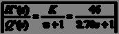
From inspection at the data,  ≈ 270 min.

The process gain is calculated as:

The estimated process model is:

(b) Nonlinear regression

By using deviation variables, the first order tank can be expressed as

The inlet flow rate is quickly changed from 1.5 gallon/min to 4.8 gallon/min so it is a step change, Q’(s) 3.3/s:

Apply the inverse Laplace transform:

By using EXCEL, the estimated model is: A comparison of the data and the two models is shown in Fig.S7.8.

The Sum of Squared Errors for the two models are:

SSE (63.2%) = 0.75

Fig.S7.8. Acomparisonofthestepresponsesofthedataandthetwomodels.

SSE (NR) = 0.43

As indicated in Fig.27.8, both methods fit the data well. The NR model is preferred due to its smaller SSE value.

Thus the transfer function can be written as:

From (5-45) and (5-46) or by factoring (e.g., using MATLAB command ) gives:

Assume that T() = T(13) = 890 C. The steady-state gain K is the change in output divided by the change in input:

K = 890 – 850 950 – 1000 = – 0.8 C/cfm

Assume that the input change in air flow rate is made at t = 2+ min so that the observed input first changes at t = 3 min ; the output first changes at t = 5 min. This means that the time delay is two sampling periods, i.e.,  = 2 min. Why is =2 min, rather than 3 min? To understand this point, first consider a process with no time delay (=0). For a step change at t = 2+ min, the first observed changes in the input and the output of this undelayed would occur at t = 3 min, because the output cannot change simultaneously due to the process dynamics. But for our process, the first changes are observed at t = 5 min which implies that

Time constant  can be obtained from the 63.2% response time:

63.2% = 850 C + (890 – 850 C)(0.632) = 875.3 C

Interpolating between t = 7 min and t = 8 min gives

Then

63.2% =

+

+ t(0) where t(0)=3, the time when the input first changes. Thus

a) Replacing  by 5, and K by 6 in Eq. 7-34

b) Replacing  by 5, and K by 6 in Eq. 7-32

In the integrated results tabulated below for t = 0.1, the values are shown only at integer values of t, for comparison. Table S7.11 Integratedresultsforthefirstorderdifferentialequation

Thus t = 0.1 does improve the finite difference model making it a more accurate approximation of the exact model.

To find 1a and 1b , use the given first order model to minimize

Substituting into expressions for 1a  and 1b gives

1a = 0.8187 , 1b = 1.0876

The fitted model is

( 0876 1 ) ( 8187 0 1) ( ykykxk

)

Let the first-order continuous transfer function be,

For Eq. 7-34, the discrete model is

Comparing Eqs. 1 and 2, for t=1, gives

 = 5 s and K = 6 volts

Hence, the continuous transfer function is

The first-order, discrete-time model is:

To find

b , use this model to minimize

where y(k) denotes the data. Thus,

Figure S7.12. Responsesofthefittedmodelandthedata

Solving simultaneously for

and

b gives

Substitutingthe data in Table E7.12 gives,

Using the graphical (tangent) method of Fig.7.5

The response to unit step change for the first-order model given by,

A comparison of the models and the data is shown in Fig. S7.13.

a) For the model in (1), the least squares parameter estimates are given by

1212 ()(1)(2)(1)(2) ykaykaykbukbuk 

Next, we generate model predictions for the calibration data (dataset basal1) using past inputs and past model predictions, but not past output data.

Figure S7.14a compares the calibration data and the model predictions, where y = y - y(0). Metric S denotes the corresponding sum of squared errors,

Figure S7.14a. Comparisonofmodelpredictionsandcalibrationdataforthe2nd orderdiscrete-timemodel(SisthesumofsquarederrorsinEq.2).

b) The comparison of the validation data (dataset basal2) and the corresponding model predictions is shown in Figure S7.14b.

b) Now, consider the first-order transfer function model

First, determine the steady-state gain, K = Δy/Δu. The output finally reaches a new steady state of about 250 mg/dL. For dataset basal1, the input change is u=2.5 units/day. Thus,

day 100 2.5dL units

To identify time constant τ, determine the time at which 63.2% of the total change has occurred. This corresponds to the time at which the output, Δy has a value of - 250 × 63.2% = - 158. For inspection of the data, τ = 134 min when y= 158 mg/dL.

The model predictions for the model in (3) can be calculated from the step response for a first-order transfer function in (5-18)

The input step sizes are M = 2.5 units/day for basal1 and 1.5 units/day for basal2

Figure S7.14b. Comparisonofmodelpredictionsandvalidationdataforthe2nd orderdiscretetimemodel(SisthesumofsquarederrorsinEq.2).

Figures S7.14c and S7.14d show the model predictions for the calibration and validation data, respectively.

c) Discussion of results

Table S7.14 lists the calculated values of S for the two models.

Figure S7.14c. Comparisonofthemodelpredictionsandcalibrationdataforthe 1stordertransferfunction(SisthesumofsquarederrorsinEq.2).

Figure S7.14d. Comparisonofthemodelpredictionsandvalidationdataforthe 1stordertransferfunction(SisthesumofsquarederrorsinEq.2).

7.15

The discrete-time model is more accurate than the transfer function model for the calibration data, which is not surprising because the former has more model parameters. Although, the transfer function model is more accurate for the validation dataset, neither model is very accurate for this dataset.

a) Fit a first-order model:

Let y = hydrocarbon exit temperature, THC u = air flow rate, FA

Note: There is a typo in the 1st printing. The step change in u should start at 17.9 m3/min, not 17.0 m3/min.

The step response data is shown in Fig. S7.15a. The step change in u from 17.9 to 21 m3/min occurs at t = 14 min. By inspection of the noisy y data, the time delay is approximately = 4 min.

Table S7.14. Average squared error for the model predictions.

Figure S7.15a. Stepresponsedataforthefurnacemodule.

From the step response data, the following information can be obtained:

From the figure,

Thus, the transfer function model is:

b) Fit a second-order model:

From inspection of the data,

Thus the second-order transfer function can be written in standard form as:

c)

d) Discussion

The model comparisons in Fig. S7.15b indicate that the two models are very similar and reasonably accurate. However, the low-order transfer function models fail to capture the higher order dynamics of the physical furnace model that was used to generate the step response data. The first-order model has a lower value of the least squares index, S:

First order model: S = 1.71 x 104

Second-order model: S= 2.01 x 104

Figure S7.15b Comparisonoffurnacestepresponsedataandmodelresponses.

(a) Fit a FOPTD model to the column step response data:

Let y = distillate MeOH composition, xD u = reflux ratio, R

The step response data is shown a in Fig. S7.16a with the step change in u from 1.75 to 2.0 occurring at t = 3950 s. By inspection of the noisy data, the time delay is 

50 s.

The following information can be obtained from the step response data:

Figure S7.16a. Stepresponsedataforthecolumnmodule.

From the figure,  = t63.2 – t(0)= 5050 – 3950 - 50 ≈ 1050 s. Thus, one estimate of the time constant is  = 1050 s. A second estimate can be obtained from the settling time, ts ≈ 7600 – 3950 = 3650 s. Thus,  ≈ ts/4 = 912 s. Averaging these two estimates gives:

Thus the identified transfer function is,

(b) SOPTD model: Use Smith’s method:

y20 = 0.85 + (0.2)(0.03) = 0.856

y60 = 0.85 + (0.6)(0.03) = 0.868

From the step response data:

t20 ≈ 4280 – 3950 – 50 = 280 s

t60 ≈ 4900 – 3950 – 50 = 900 s

From Fig. 7.7:

The SOPTD model can be written as:

which can be factored using (5-45) and (5-46):

d) Discussion

The model comparisons in Fig. S7.16b indicate that both models are reasonably accurate. However, the second-order model is more accurate as indicated visually and by its slightly lower S value:

First order model: S = 9.014 x 10-4

Second-order model: S= 9.012 x 10-4

Fig. 7.16b. Comparisonofcolumnstepresponsedataandmodelresponses.