An econometric model for Linear Regression using Statistics
Renvil Dsa1, Remston Dsa2Abstract - This research paper discusses the econometric modeling approach of linear regression using statistics. Linear regression is a widely used statistical technique for modeling the relationship between a dependent variable and one or more independent variables. The paper begins by introducing the concept of linear regression and its basic assumptions.

The univariate and multivariate linear regression models are discussed, and the coefficients of the regression models are derived using statistics. The matrix form of the Simple Linear Regression Model is presented, and the properties of the Ordinary Least Squares (OLS) estimators are proven. Hypothesis testing for multiple linear regression is also discussed in the matrix form.
The paper concludes by emphasizing the importance of understanding the econometric modeling approach of linear regression using statistics. Linear regression is a powerful tool for predicting the values of the dependent variable based on the values of the independent variables, and it can be applied in various fields, including economics, finance, and social sciences. The paper's findings contribute to the understanding of the linear regression model's practical application and highlight the need for rigorous statistical analysis to ensure the model's validity and reliability.
Key Words: econometric model, linear regression, statistics, univariate regression, multivariate regression, OLS estimators, matrix form, hypothesis testing.
1. INTRODUCTION
Linear regression is a powerful statistical modeling techniquewidelyusedtoanalyzetherelationshipbetween a dependent variable and one or more independent variables. In a simple linear regression model, the dependent variable is assumed to be a linear function of one independent variable, while in a multiple linear regression model, the dependent variable is a linear functionoftwoormoreindependentvariables.
The coefficients of the linear regression model are represented by beta (β) values, which are constants that determine the slope and intercept of the regression line.
The beta values are estimated using the Ordinary Least Squares (OLS) method, which involves minimizing the sum of squared errors between the predicted values and theactualvaluesofthedependentvariable.
Thematrixformofthelinearregressionmodel isa useful tool for understanding the relationship between the dependent and independent variables. The matrix form allows for a more efficient calculation of the beta values andthevariance-covariancematrixofthebetavalues.
Partial derivatives are used to derive the expected values and variation of the beta values. The expected values of the beta values are equal to the true beta values, and the variation of the beta values can be used to derive confidence intervals and hypothesis tests for the beta values.
The relationship between the beta values and the normal distribution is important in understanding the properties of the OLS estimators. The beta values are normally distributed, and their variance-covariance matrix can be usedtoderiveconfidenceintervalsandhypothesistests.
Hypothesis testing is an essential component of linear regression analysis. The null hypothesis is typically that the beta value is equal to zero, indicating that there is no relationship between the independent variable and the dependent variable. The t-test and F-test are commonly usedtotesthypothesesaboutthebetavalues.
The ANOVA matrix is a useful tool for decomposing the total variation in the dependent variable into the explained variation (sum of squared regression) and unexplainedvariation(sum ofsquared error). Thesum of squared total is the sum of squared deviations of the dependentvariablefromitsmean.
The relationship between the sum of squared regression, sum of squared error, and sum of squared total with the mean squared error and the degrees of freedom is important in interpreting the results of the linear regressionanalysis.
In summary, linear regression is a powerful statistical modeling technique that can be used to analyze the
relationship between a dependent variable and one or moreindependentvariables.Thebetavalues,matrixform of the model, partial derivative concept, expected values and variation of beta values, relationship with normal distribution, hypothesis testing, ANOVA matrix, formulas forsumofsquared regression,sumofsquared error,sum of squared total, and relationship with mean squared error, t-test, and F-test with degrees of freedom are importantconceptsinunderstandingandinterpretingthe resultsoflinearregressionanalysis.
2. METHODS
2.1 Deriving the coefficient of the regression model for the simple linear regression model
Theimportantresultthatisneededtoderive ̂ and̂
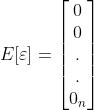
Suppose, is the sample mean of y then is defined as 1 overntimesthesummationfromi=1tonof
Italsomeansthat isequaltothesummationfrom i=1tonof
∑ (a)
Similarly, isthesamplemeanofyandisdefinedas1overntimes thesummationfromi=1tonof
Italsomeansthat isequaltothesummationfrom i=1tonof =∑ (b)
There are some important results that we need to know usingthesummationoperator,
The written L.H.S. can also bewrittenas:
Table 1: Different forms of ∑ ( - )( - ) [1]
Derive
Fromequation(a)andequation(b) =∑ - + -
[Equation(1)]
Derive:∑ =∑ ( - )
L.H.S.
Fromequation(b)
Applying Partial Derivative with respect to
Fromequation(a)
Deriving the formula for ̂ and ̂ [2]
1. S.S.E: The sum of squared error is equal to the summation from i = 1 to n of the square of the difference between and ̂
2. istherealobservationand ̂ isthepredicted observation
3. The goal is to minimize the distance between the realobservationandthepredictedobservation.
4. The equation is a quadratic equation and the objective is to find the minimum point and not the maximumpoint.
S.S.E
Applying Partial Derivative with respect to ̂
(
̂ ) (-1)
Tofindthemaximaorminima, Equivalently,thederivativeequals0.
Tofindthemaximaorminima, Equivalently,thederivativeequals0.
fromequation(a)andequation(b)
Scalar
ForY, theintercept, istheslope,and is the error term epsilon. This is known as the scalar form. Suppose therearendatapoints, thenirangesfrom1ton
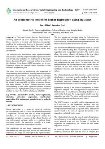
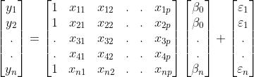
TheMatrixFormofYis
Here,
2.3 SLR Matrix Form Proof of Properties of OLS(Ordinary Least Squares) Estimators
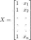
The first assumption is that the expected value of epsilon isequaltozeroforalliandtheseiareintherangeofi=1, 2,...,n,wherenisthenumberofdatapoints.
Themathematicalrepresentationisstatedbelow.
E[ ]=0 i,wherei=1,2,3,...,n.
Theanticipatedvalueofvectorepsilonisgoingtobezero vector or in rows, so it's essentially epsilon, the expected value of epsilon is going to be simply a vector of zero, wheretherewillbenrows,Sothisisthefirstassumption that will be evaluated when working with the simple linearregressionmodelinmatrixform.
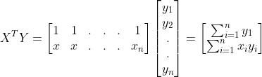
Expected value and Variance of [4]
E[ ]=
The second assumption is about the variance of the epsilon
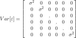
Var[] i. The epsilon vector's variance matrix is equal to sigma squared times the identity matrix, with dimensions ofnbyn.
Sothevarianceofepsilonisequaltosigmasquaredonall diagonal terms up to n rows, and all these entries should bezerootherthandiagonalterms.
Var[ ]= I
The third assumption is that the epsilon values are uncorrelated. If they are uncorrelated then that means that for any Epsilon values and , the variance of and is equal to zero. This also means that the covariances of and are equal to zero. Thus, wherei j,thecovarianceof and isequaltozero.
As ’sareuncorrelated
The mathematical representation of the above third assumptionis:
Var( )=0
Cov( )=0
Cov( )=0 i
Astheepsilonofi's( ’s)areuncorrelatedwitheachother, and based on these three assumptions, when combined with the fourth assumption, allow for a very good powerful construction of the simple linear regression model,fromwhichvariousresultscanbederived.
Thefourthandlastassumptionisthattheerrortermsare normallydistributed.
The epsilon i( ) follows the normal distribution with somemean( )andsomevariance( ).
N( , ) [5]
From Assumptions 1 and 2, we know that = E[ ] = and Var[ ] = where is the standard deviation. Also,fromassumption3where i,wherei=1,2,3,.........,n Cov( ) = 0 i which means these epsilon are independentandareidenticallydistributed.
Hence, N( , )
Hence, =Ŷ = Ŷ
Derive and show that E[ ̂] =
As ̂ =
E[̂]=E[ ]
Note: isnotstochastic,it’snotrandomatall,it is all just constant known values that are multiplied by eachother.
E[̂]= E[ ]
As,Y=X +
E[Y]=E[X + ] =E[X ]+E[ ] =E[X ] (FromAssumption1,E[ ]=0) =X
Hence, E[̂]= E[ ] = ( X)
As ( X)= where Xissymmetricmatrix
E[̂]=
E[̂]=
Derive and show that Var[ ] =̂
Var[ ̂]=Var[ ]
LetB= Var[B ] = BVar[ ] = BVar[X + ] = BVar[ ] +BVar[ ]
Here, in Var[ ] is not random and continuous hence wecanassumethatVar[ ]=0
FromAssumption2whereVar[ ]= I
Var[ ̂]=B I = I
As issymmetric, =X = X
Var[ ̂] = I = IX
As ( X)= where Xissymmetricmatrix
I
As are unobservable, cannot be computed hence we assume ̂isanestimatorof
Hence,Var[ ̂]=̂
2.4 Hypothesis testing for Multiple Linear Regression- Matrix form
Y=X
here, = Ŷ where Y above inthe equationis the actual observationand ̂ isthefittedobservation.
The following equation gives the sum of squared errors(SSE):
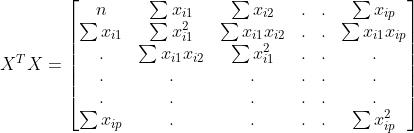
SSE=̂
Therefore,theabovefunctioncanbewrittenas:
SSE= ̂ ̂
Tofittheregressionmodel,thegoalshouldbetominimize theSSE, minimize(SSE)=minimize(̂ )
=minimize[ ̂ ̂ ]
Here, ̂ = where E[̂]= Var[̂]=̂ ̂ ̂ = ̂ =MSE= = ̂
Here, p regressors of interest 1 is for and n is the numberofsamplesinthepopulation
LetSebetheStandardError
Hence, Se(̂)=√ ̂ ̂ =√̂
Here,Se(̂ )=√̂
Hypothesis
Hypothesis testing on a linear combination of regression parameters in the matrix form of the linear regression problem.
Belowis the general formula ofthe regressionmodel that isinmatrixform:
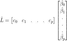
Y=X
Scalarrepresentationoftheregressionparameters:
Y= + + + +……….+
Linear
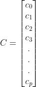
The , , ,...., intheaboveequationrepresentthe constants.
Hypothesis to be tested: : ̂ = vs : ̂
Expectedvalueof ̂ :
E[ ]=E[̂ ]= E[ ]= =L
istherowvectoroftheconstants.
Varianceof ̂ : ̂ = = c= ̂ c
Formulation of the test statistics is a t-test where the parameter of interest (̂) follows the normal distribution withmeanofLandvarianceof ̂ c.
̂ N( , ̂ c)
TeststatisticsT:
T =
:Itisthevalueofthelinearcombinationunderthenull hypothesis
where =√̂
Thenteststatisticsbecomes,
T= √̂
ANOVAMatrixForm[7]:
SSR:SumofsquaresRegression:∑ (̂ )
SSE:SumofsquaresErrors:∑ ̂
SST:SumofSquaredTotal:∑ ( )
Source of variation Sumof Squares degree sof freedo m
Mean Square F statistic
Regresion SSR p MSE= F=
Errors SSE n-p-1 MSE= = ̂
Table 2: ANOVA matrix form [8]
F= Hypothesis to be tested: : = = = =...= vs : F [9]
f F> thenreject elseaccept
3. CONCLUSIONS
In conclusion, this research paper has explored the econometricmodelingapproachoflinearregressionusing statistics. The paper has presented the fundamental concepts of linear regression, such as the basic assumptions and the definition of the dependent and independentvariables.
The paper has then discussed the univariate and multivariatelinearregressionmodels,andthecoefficients of the regression models have been derived using statistical methods. The matrix form of the Simple Linear Regression Model has been presented, and the properties oftheOrdinaryLeastSquares(OLS)estimatorshavebeen proven.
Finally, the paper has discussed hypothesis testing for multiple linear regression in the matrix form. The importance of understanding the econometric modeling approach of linear regression using statistics has been emphasized, and the paper's findings contribute to the understanding of the practical application of the linear regressionmodel.
Overall,linear regression is a powerful tool for predicting the values of the dependent variable based on the values of the independent variables. It can be applied in various fields, including economics, finance, and social sciences. Rigorous statistical analysis is necessary to ensure the model's validity and reliability, and this paper has provided insights into the statistical methods used in linearregressionmodeling.
REFERENCES
[1] Introduction to Linear Regression Analysis, 5th Edition"byMontgomery,Peck,andVining
[2] AppliedLinearRegression,3rdEdition"byWeisberg
[3] MatrixApproachtoSimpleLinearRegression"byKato andHayakawa
[4] Linear Regression Analysis: Theory and Computing" byLiuandWu
[5] LinearModelswithR,2ndEdition"byFaraway
[6] Applied Regression Analysis and Generalized Linear Models,3rdEdition"byFox
[7] StatisticalModels:TheoryandPractice"byFreedman, Pisani,andPurves
[8] StatisticalInference"byCasellaandBerger
[9] Probability and Statistics for Engineering and the Sciences,9thEdition"byDevore