

Dynamic Targeting to Improve Earth Science Missions
Alberto Candela, Jason Swope, Akseli
Kangaslahti, Itai Zilberstein, Qing Yue, Steve Chien
ai.jpl.nasa.gov
Northeastern University
01 April 2024
Reference herein to any specific commercial product, process, or service by trade name, trademark, manufacturer, or otherwise, does not constitute or imply its endorsement by the United States Government or the Jet Propulsion Laboratory, California Institute of Technology.
© Copyright 2024, California Institute of Technology, All Rights Reserved. This research was carried out by the Jet Propulsion Laboratory, California Institute of Technology, under a contract with the National Aeronautics and Space Administration. JPL CL #23-3071 #23-4890.

Introduction
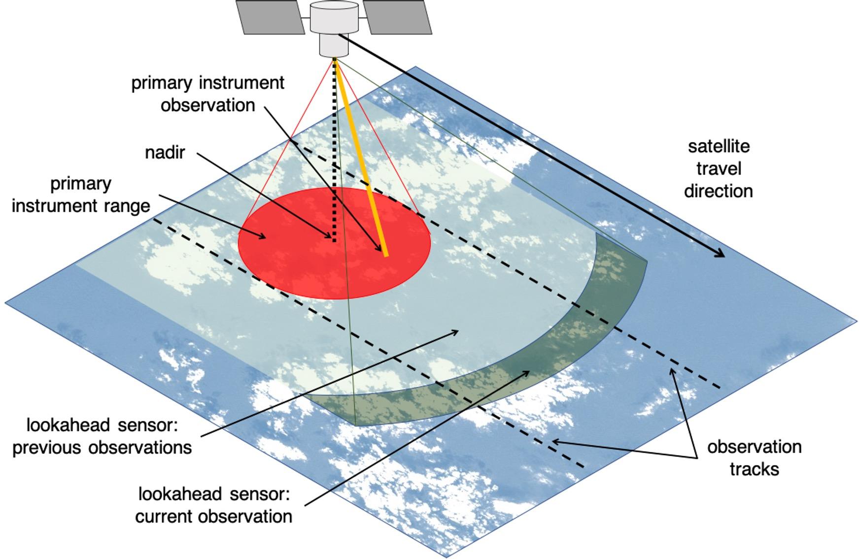
• Remote sensing: high spatial resolution can be expensive and physics dictates trades of footprint versus spatial resolution. Often instrument configuration can be optimized to target.
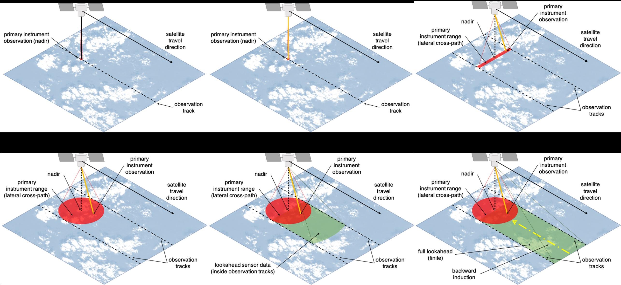
• DT uses information from a lookahead sensor to identify targets for the primary, pointable sensor to improve science yield
• Dynamic targeting (DT) can improve the science return of swath/mode limited instruments

• We advocate DT to become commonplace across many future Earth Science missions
jpl.nasa.gov 3
Related Work: Cloud Avoidance
• JPL Mission (Thompson et al., 2014): Rapid spectral cloud screening (compression) for AVIRIS airborne instrument
• JAXA - L3Harris Mission (Suto et al., 2021): cloud avoidance for TANSO -FTS-2 thermal and near infrared carbon observations
• JPL Study (Hasnain et al., 2021): Greedy, graphsearch, DP algorithms for agile spacecraft imaging of clear vs. cloudy skies (binary)
jpl.nasa.gov 4
Hasnain et al., 2021
Initial Work: Hunting Deep Convective Storms
• NASA Study: Smart Ice Cloud Sensing (SMICES) satellite concept
• Dynamic measurements of different storm clouds categories
• Swope et al. 2021: greedy heuristics
❖ This work is a continuation and generalization of the SMICES concept
jpl.nasa.gov 5
Swope et al., 2021
1. Use Cases
2. SMICES ML
3. Simulation Studies: SMICES: Storm Hunting
Global Studies: Storm Hunting Cloud Avoidance
4. Dynamic Targeting: Problem Definition Algorithms
5. Experiments and Results
6. Conclusions and Future Work
jpl.nasa.gov 6
Overview
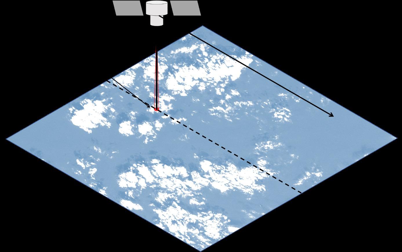
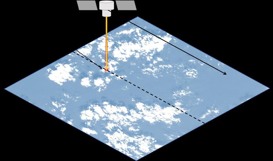
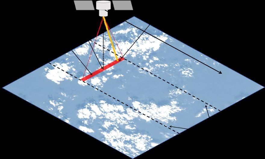
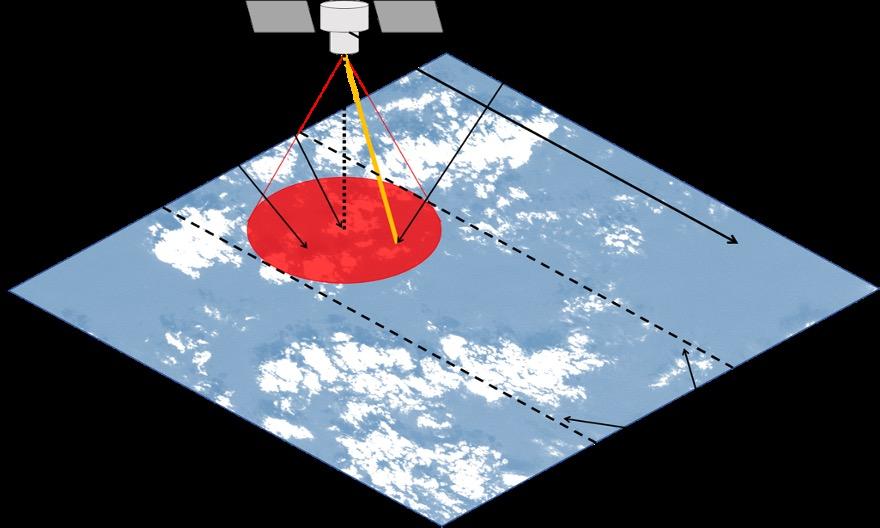
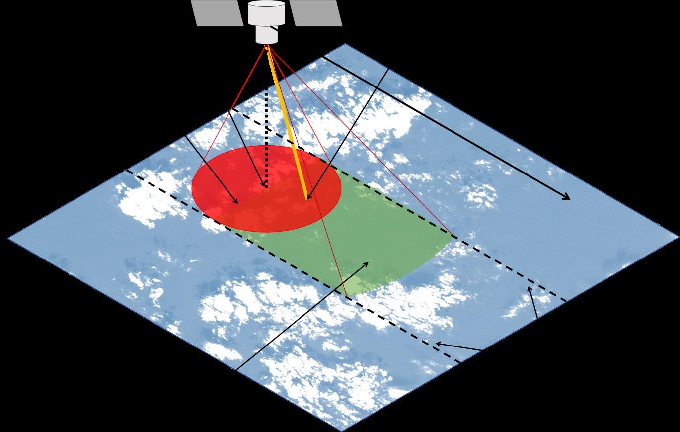
Example Concept: Cloud Avoidance
• Many instrument concepts do not “like” clouds
• Example: OCO-3 clouds interfere with CO 2 retrieval
• lookahead visible or IR camera → detect clouds
• OCO-3 PMA targets around clouds
• Example: VSWIR spectrometers imaging surface (same)
detect and avoid clouds
trajectories
jpl.nasa.gov 7
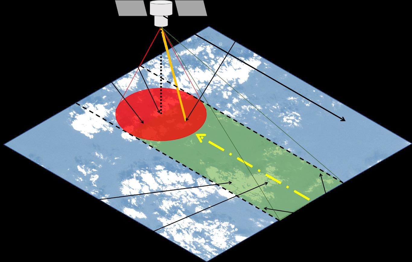
Example Concept: Planetary Boundary Layer (PBL)
• PBL phenomena can be rare and short-lived
• Instrument to detect likely PBL areas
• Sounder at 118 and 138 Ghz (low resolution) to detect areas of high gradient in temperature and moisture*
• Instruments to study are narrow FOV sensors
• Differential Absorption Radars for opaque (cloudy) areas **
• Differential Absorption Lidar for clear-air areas***
* TEMPEST-D, HAMSR, MASC heritage
** Differential Absorption Radar eg. VIPR
*** Differential Absorption Lidar
identify areas of likely PBL phenomena based on high gradient in moisture and temperature
trajectories
jpl.nasa.gov 8
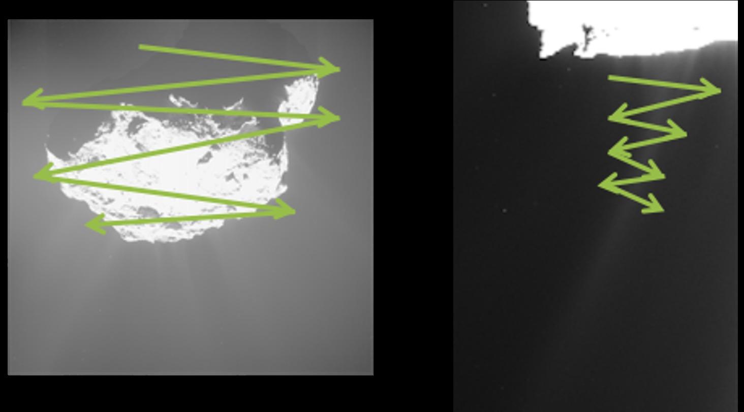
For Rosetta Orbiter mission, observations were planned weeks to months in advance. (wide FOV: OSIRIS, narrow FOV MIRO)
(Non Terrestrial) Example Concept: Plume Study trajectories
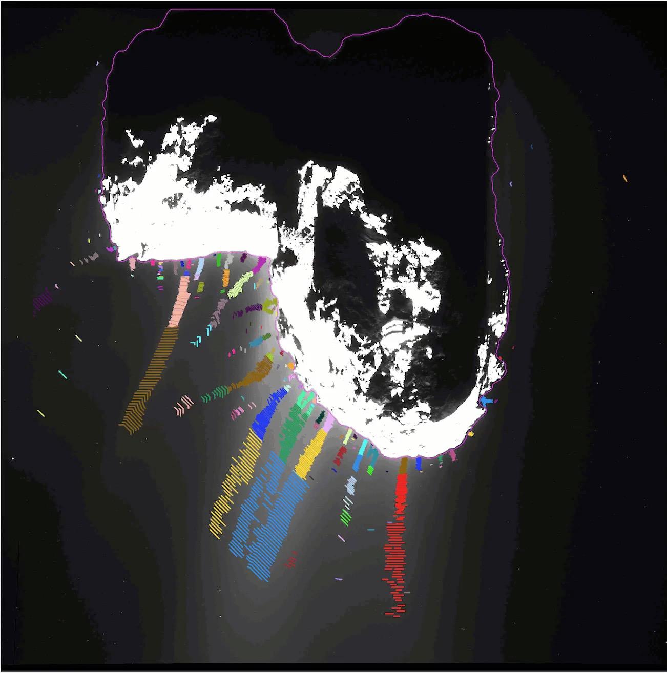
Future missions could dynamically track plumes and execute targeted sweeps across plumes to sample at much higher temporal frequency. See Brown et al. 2019 Astronomical J.
Note that in these use cases primary instrument data could be used in near real-time to identify the edge of the feature!
jpl.nasa.gov 9
Terrestrial Plumes
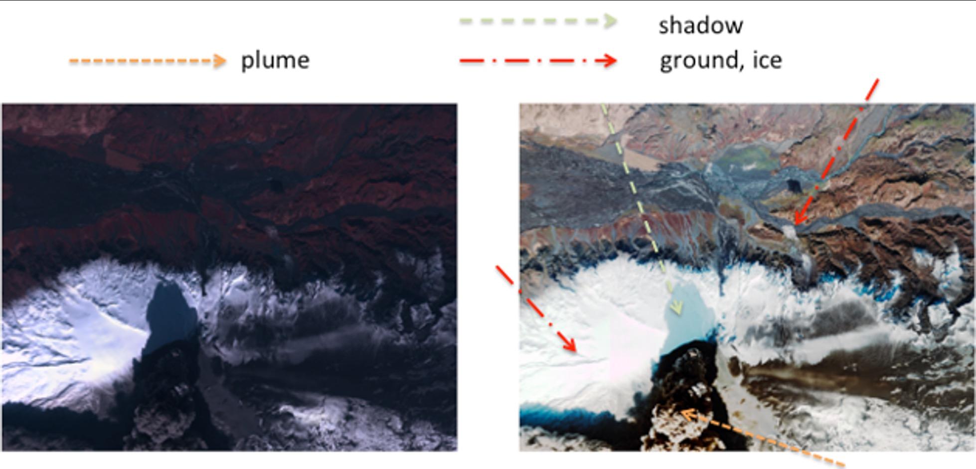
WorldView -2 Image of Eyjafjallajökull eruption, acquired April 17, 2010
10
jpl.nasa.gov
Machine Learning
● SMICES: Storm Hunting
jpl.nasa.gov 11
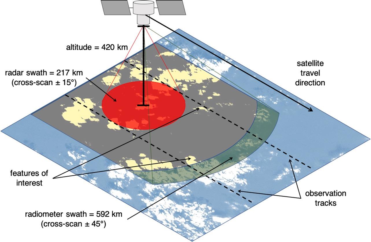
Concept: SMICES
• NASA ESTO mission concept
• Reconfigurable, smart instrument combining:
• *Radiometers (lookahead): up to 45 °
• **Radar (primary): up to ±15°
• SMICES would use AI for:
• instrument calibration
• primary instrument on/off and targeting:
• radiometer → likely deep convective ice storm
• radar → on/off and targeting
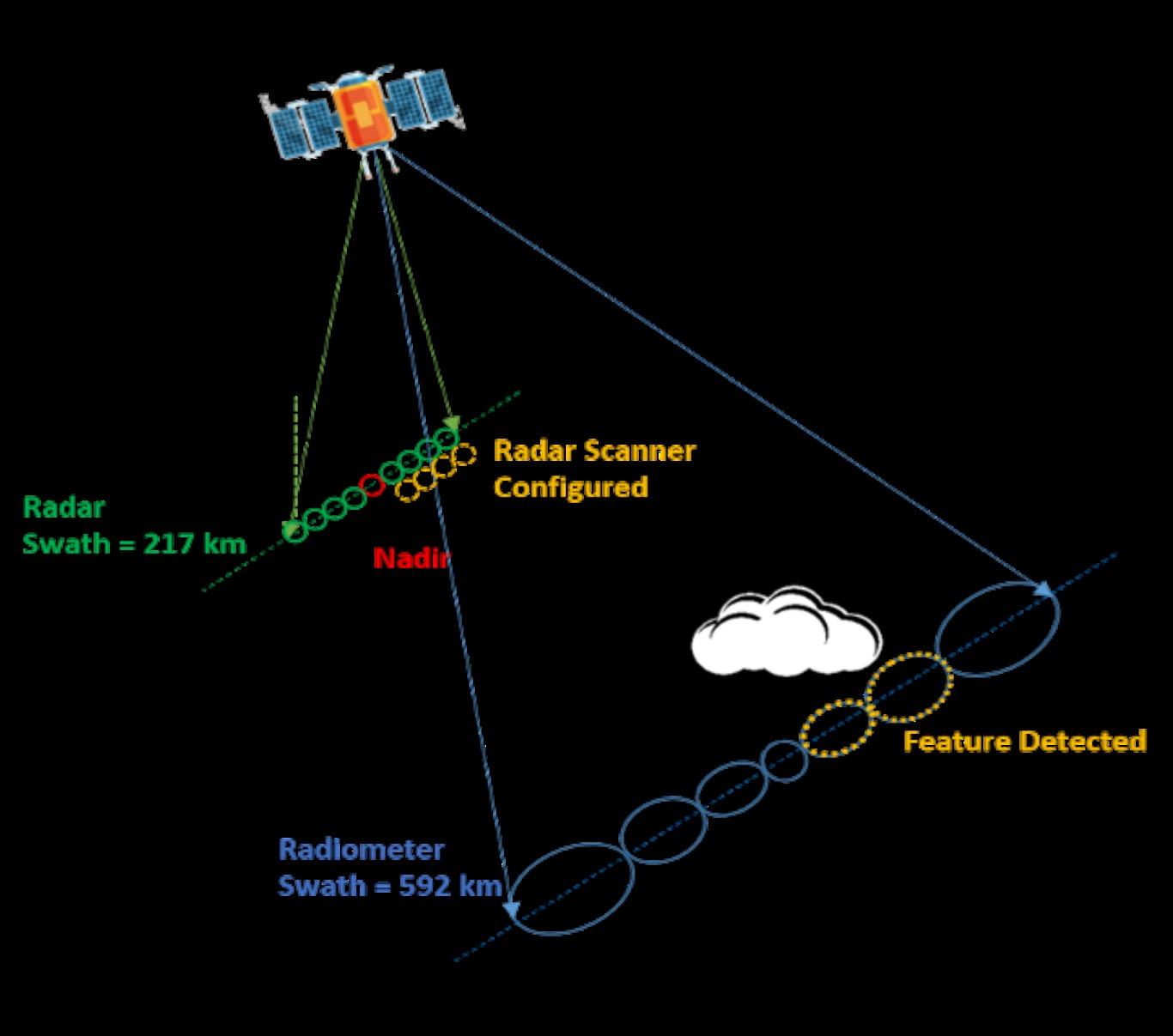
Bosch-Lluis et al., 2020
Machine Learning: How to detect deep convective ice storms in Lookahead Radiometer Data?
trajectories
* TWICE heritage ** ViSAR heritage
jpl.nasa.gov 12
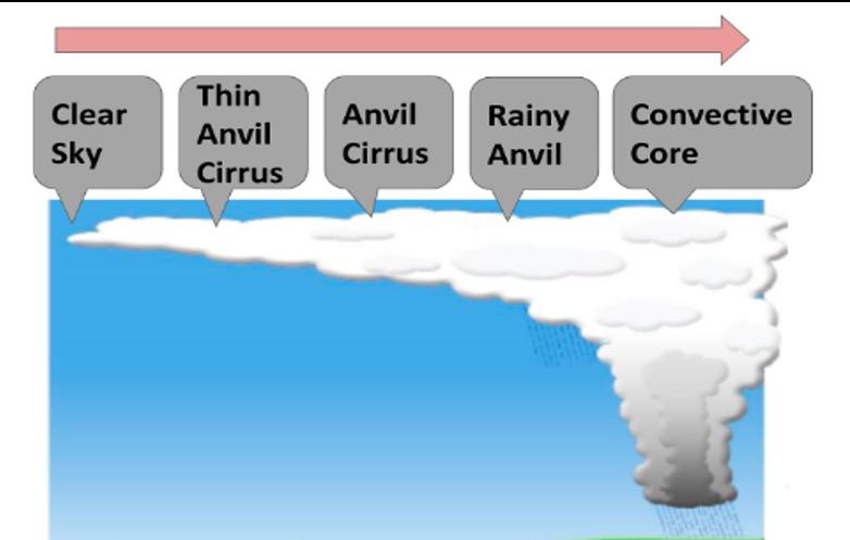
Targets of Interest
* Methods apply to other foci! e.g. we can focus on anything that is detectable. DIffering science campaigns, operating modes, etc.
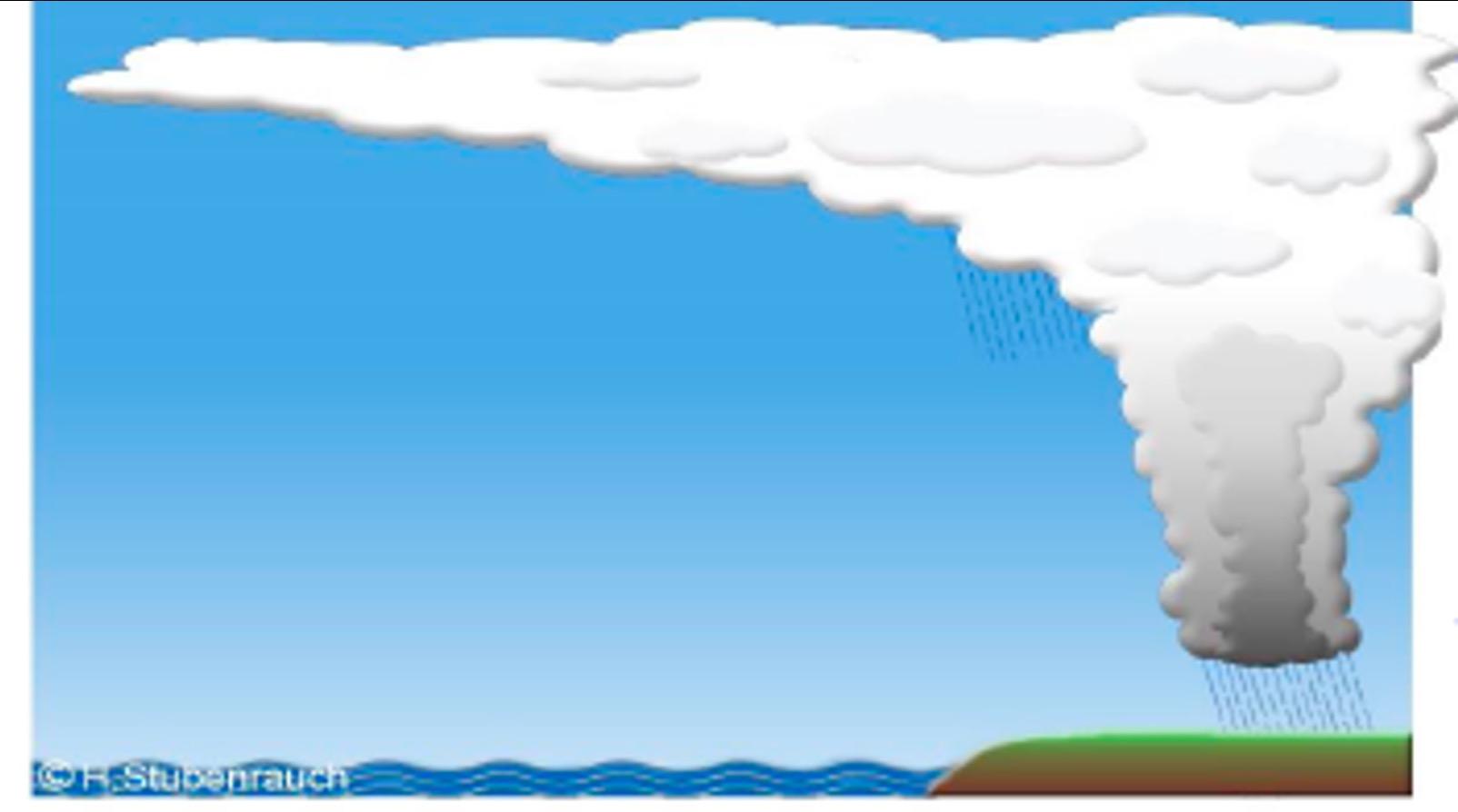
Clear Sky Thin Anvil Cirrus Anvil Cirrus Rainy Anvil Convective Core Increasing Interest* 13
The Problem of Data Labels
• For classification problems, how to get labels for data?
• Really, really don’t want to manually label…
• We use atmospheric simulation as “Digital Twin” (Questions? see Qing Yue)
• Digital Twin - software artifact of physical system for advantage e.g.
https://www.ge.com/digital/applications/digital -twin
• Access to hidden variable(s)
• Ability to generate massive amounts of training data (or run at faster than real-time)
• Ability to generate hard data (such as infrequent failures, risk to life/hardware)
14
Simulated Storm Data
• 2 Regions Simulated Storm Datasets
• Tropical (Carribean )
• 13 images each 119x208 pixels with 15km pixels spatial extent of 1,785km x 3,120km 13 x 1h intervals
• Non-Tropical (East Coast US)
• 29 image cutouts each1998x270 pixels with 1.33km pixels for a spatial extent of 2,657km x 359km. 3 x 12h intervals
1. Can simulate target environmental conditions
2. Can simulate hidden variables (e.g. hard/impossible to sense quantities)
3. Can simulate both radiometer and radar data
15
Clustering to avoid Labelling Problem
• Take “Digital Twin” weather simulation data
• Cluster* based on hidden variables:
• Particle Size
• Cloud Top Height
• Ice Water Path
• Use hidden variable statistics on derived clusters to map clusters → classes
• Convective Core
• Rainy Anvil
• Anvil Cirrus
• Thin Cirrus
• Clear Sky
* Use k-means clustering (unsupervised learning) which attempts to:
- maximize within cluster coherence; and
- maximize between cluster separation.
• Use cluster labels as class labels (human expert mapped)
16
Cluster Mapping
Hidden values by cluster Data Visualization
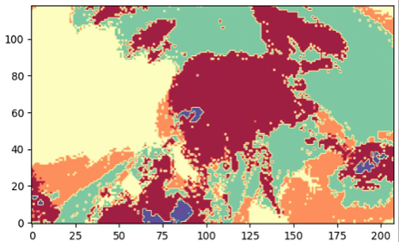
Tropical GWRF data set labelled by derived clusters
● Higher value targets (Convection Core, Rainy Anvil) exhibit:
○ Larger Ice Water Path (IWP)
○ Larger Median Particle Size
○ Lower Median Cloud Top Height
24,752 data points 17 Cluster → Label/Class mapping based on science input!
Cluster Color IWP (mean: std) Median Particle Size (mean: std) Median Cloud Top Height (mean: std) Assigned Cloud Type Yellow 0: 0 0: 0 0: 0 Clear Orange .98: 12.9 37.2: 16.5 11,794: 1,290 Thin Cirrus Green 55.2: 197 103: 37.9 7,412: 787 Cirrus Red 473: 806 270: 169 4,870: 573 Rainy Anvil Purple 8,476: 4,312 539: 155 4,539: 652 Convection Core
15 km x 15 km pixels
Impact of # of Clusters on Cluster Separation and Coherence
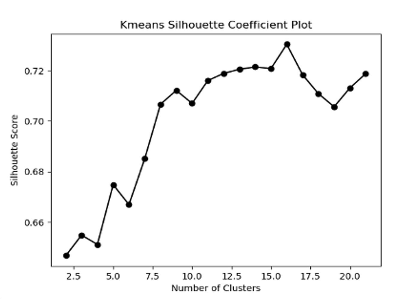
Silhouette Score:
Calculates goodness of clustering techniques
1: clusters are well distinguished
0: clusters are indifferent
-1: clusters are incorrect
Equation: (b – a) / max(a, b)
a = average intra cluster distance: average distance between each point within a cluster
b = average nearest cluster distance: average distance between the instances of the next closest cluster
● Perfectly separated clusters have a silhouette score of 1
● Local maximums at 5, 9, and 16 clusters
● Score increase is small (0.675 → 0.735 = .06) between 5 and 16 clusters
● 5 clusters provides good clustering and maps well to the 5 labels provided by the scientists (convection core, rainy anvil, cirrus, thin cirrus, clear) 18
Two Datasets
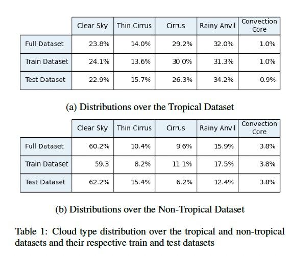
19
Learning Classifiers
• Clusters → Labels
• Present labelled data to classifier learning methods to learn: simulated instrument data
→ storm/cloud class (do NOT provide hidden variables to classifier)
• Instrument Data: 8 bands of radiance
• Tb250+0.0, Tb310+2.5, Tb380-0.8, Tb380 -1.8, Tb380-3.3, Tb380 -6.2, Tb380 -9.5 Tb670+0.0
Classification Methods applied:
1. random
2. decision forest (RDF),
3. support vector machine (SVM),
4. Gaussian Naıve Bayesian,
5. a feed forward artificial neural network (ANN),
6. and a convolutional neural network (CNN).
• The classifiers operate at the single pixel level;
• given radiometer measurements at a given pixel, what is the cloud class at that pixel.
• Thus, our current classifiers do not take into account neighboring pixel values.
• Classifier performance was evaluated using 5-fold cross-validation, and testing was performed on a separate held-out test set.
20
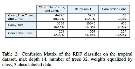
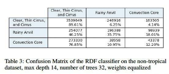
RDF
• The non-tropical dataset proved to be significantly more difficult to classify than the tropical dataset.
• The accuracy for the storm cloud classes (rainy anvil and convection core) decreased by about 2x.
• The non-storm class accuracy remained relatively unchanged when compared to the tropical dataset.
• When looking at the non -storm/storm cloud accuracy the RDF achieved 90% non-storm accuracy and 42% storm accuracy.
21
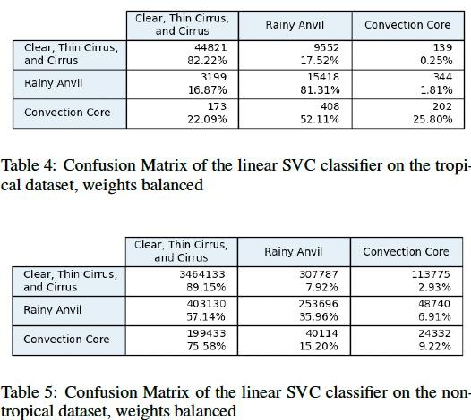
SVM/Linear SVC
• The SVM classifier performed worse in the storm classes on the non -tropical dataset than it did on the tropical dataset.
• While the non -storm classification accuracy increased to 89%, the accuracies in both storm classes decreased by more than half when compared to the tropical dataset performance.
• The storm class accuracy over the non-tropical dataset was 40%.
22
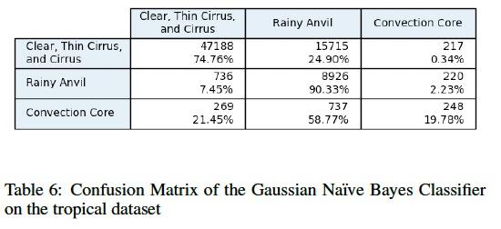
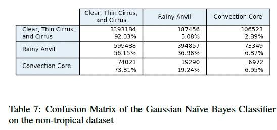
Gaussian Naïve Bayes
• The two class accuracy over the tropical dataset is 75% for non -storm and 42% for storm.
• The two class accuracy over the tropical dataset is 92% for non -storm and 55% for storm.
23
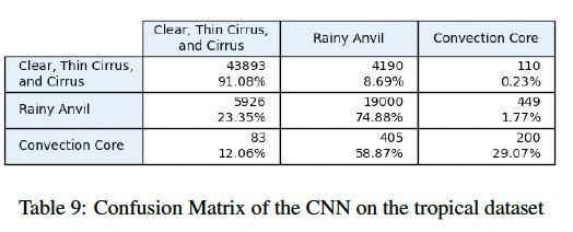
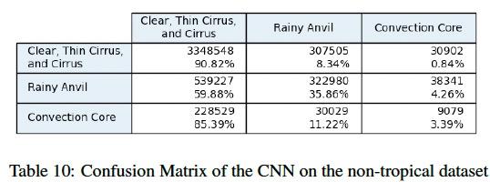
CNN
• The CNN experiences difficulty when trained on the non- tropical dataset. The heavier skew towards non- storm clouds caused the classifier to classify the majority of the test dataset as non- storm.
• The classifier achieved a 91% accuracy in non - storm clouds and a 44% accuracy in storm clouds on the non - tropical dataset.
• For future work, we plan to upsample the minority classes when training our neural networks.
24
Takeaways from the ML
• Skewed minority classes (few deep convective storms in nature) challenges for ML. (Future study)
• Non -tropical dataset challenges all of the ML techniques.
• Asymetric loss function (want to capture all deep convective storms even at cost of false alarms needs to be be better incorporated).
• Future work to incorporate contextual information (neighboring pixels) into classifiers.
• Study of other contexts to increase generality (seasonal, regional, diurnal, classifiers)
• Even at relatively low accuracy rates, classifiers can dramatically improve overall system performance (still harvest more high value targets than random).
25
Targeting Simulation Studies
● SMICES: Storm Hunting
● Global Studies: Storm Hunting, Cloud Avoidance
jpl.nasa.gov 26
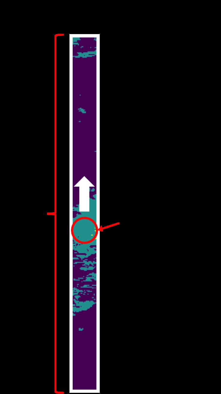
SMICES: Storm Hunting
• Continuation of previous SMICES work (Swope et al. 2021)
• Storm hunting: collect data of storm clouds
• 5 cloud classes: most interesting/scarce rainy anvil and convective core
• Data comes from the Global Weather Research and Forecasting (GWRF) state -of-the-art weather model (Skamarock et al. 2019)
• 2 datasets of high -storm regions, resolution 15 km/pixel:
• Non-tropical (U.S. Eastern Coast): 4,050 km x 29,970 km
• Tropical (Caribbean): 3,120 km x 1,785 km
• Simulated satellite mission: simple, linear, parallel trajectories
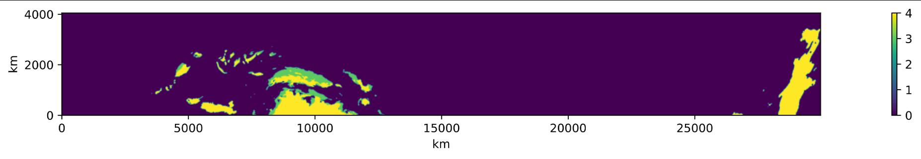
Non-tropical Tropical interest


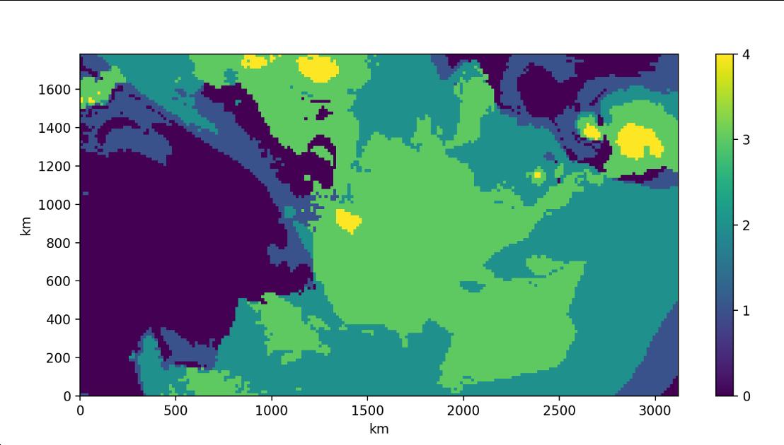
jpl.nasa.gov 27
Global Simulation Studies
• Global datasets that extend and complement the SMICES study
• Simulate more realistic satellite trajectories of Earth science missions
• 2 studies: storm hunting and cloud avoidance
Storm Hunting Cloud Avoidance
jpl.nasa.gov 28
Global Study: Satellite Trajectories
General Mission Analysis Tool (GMAT) was used to simulate realistic satellite trajectories.
Orbital parameters, Low Earth Orbit:
• Altitude: 400 km
• Period: ~95 minutes
• Inclination: 65 degrees
• Eccentricity: 0
Simulated 36,000 time steps at 1 second per time step, spanning 10 hours (~ 6 full orbits)
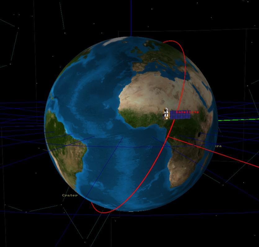

jpl.nasa.gov 29
GMAT
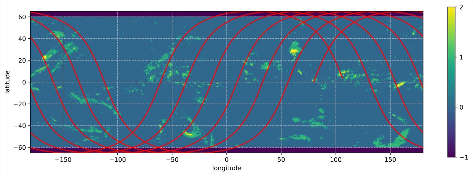
Global Study: Storm Cloud Dataset
*Merged clear sky, thin anvil cirrus, anvil cirrus
Dataset:
• Merged and aligned 2 global datasets
• Precipitation: GPM IMERG products
• IR Brightness Temperature: NOAA Climate Prediction Center/NCEP/NWES products
• Spatial res: 4 km/pixel
• Temporal res: 2 images/hour (interpolation)
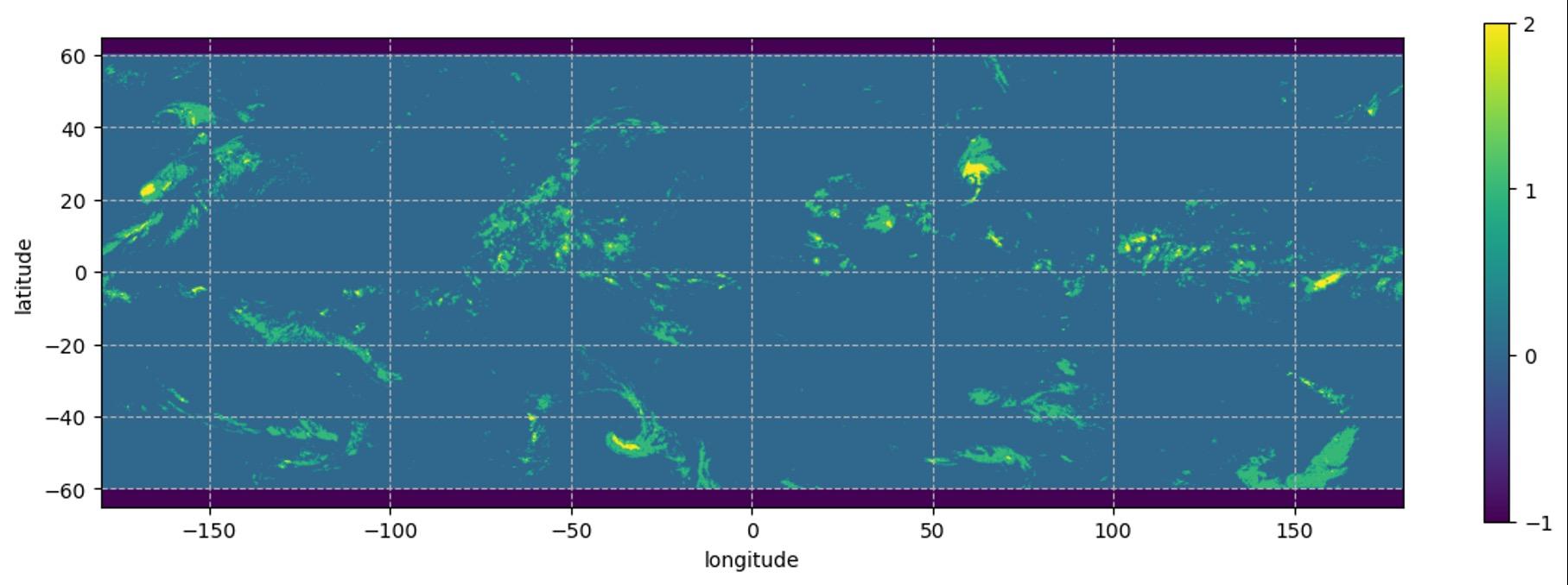
jpl.nasa.gov 30
Storm Classes Precipitation IR Bright. Temp. No storm* (0) < 5 mm/hr > 240 K Rainy Anvil (1) > 5 mm/hr > 240 K Convection Core (2) > 5 mm/hr < 240 K Importance
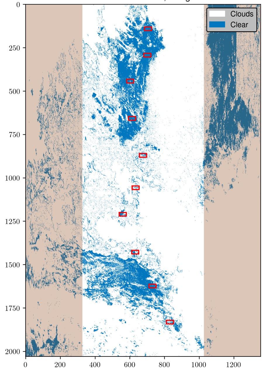
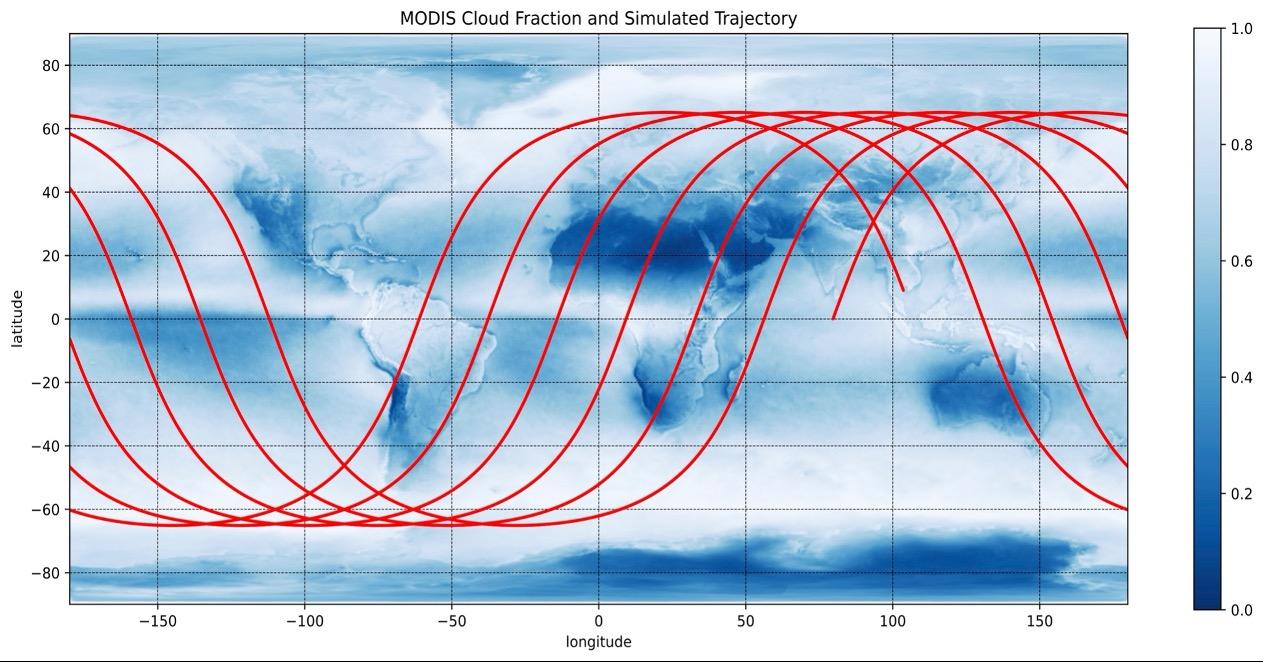
Global Study: Cloud Avoidance Dataset
Data set:
• MODIS cloud fraction global product (AQUA satellite)
• Spatial res: 0.1 degrees/pixel (~11 km/pixel)
• Temporal res: 1 image/day (interpolation)
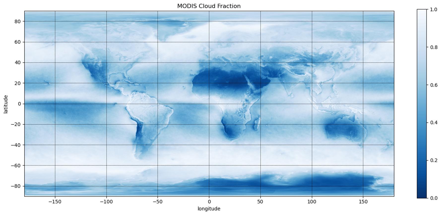
Definitions:
• Clear sky: cloud fraction < 0.35
• Mid-cloud: 0.35 <= cloud fraction <= 0.65
• Cloud: cloud fraction > 0.65
Importance
Definition: Cloud algorithms for Landsat 8 (Foga et al. 2017)
trajectories
jpl.nasa.gov 31
Dynamic Targeting
● Problem Formulation
● Algorithms
jpl.nasa.gov 32
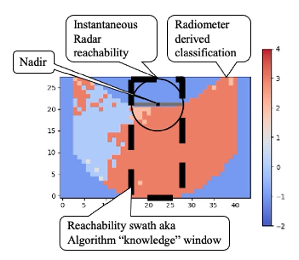
Dynamic Targeting: Problem Formulation
Pointing planning problem
● Goal: maximize observations of high -value targets (clouds) given energy constraints
● Tie-breaker: points closest to nadir are preferred
Instruments
● Lookahead sensor: radiometer, 105 -1000 km range

● Primary instrument: radar, 217 km reachability window
Energy constraints

● 20% duty cycle (radar needs to be turned off 80% of the time)
● Each radar measurement consumes 5% state of charge (SOC)
● Battery recharges 1% at each time step
jpl.nasa.gov 33
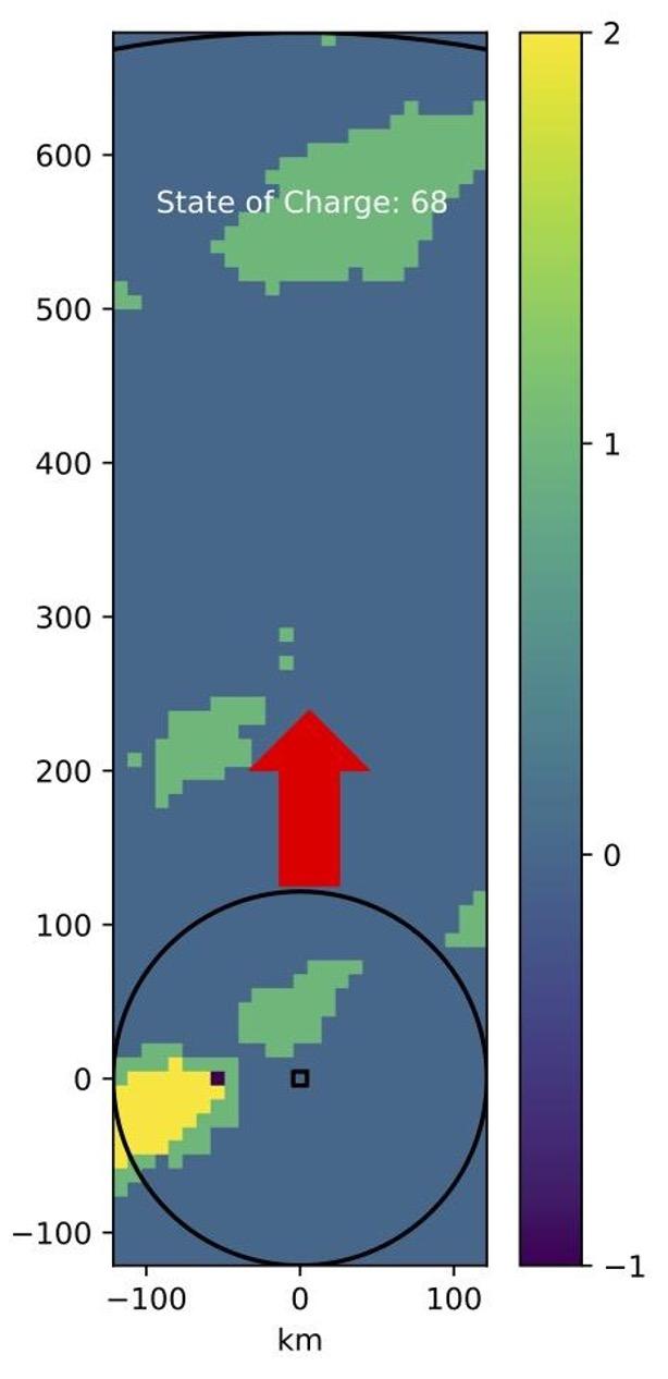
Dynamic Targeting: Example (Video)
Storm Hunting
GPM / IMERG
Dynamic Programming
2 = convection core
1 = rainy anvil
0 = no storm
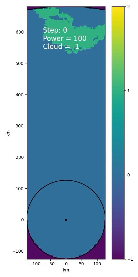
jpl.nasa.gov 34
Dynamic Targeting: Example (Explanation)
a) Energy is saved for high-value observations in the near future
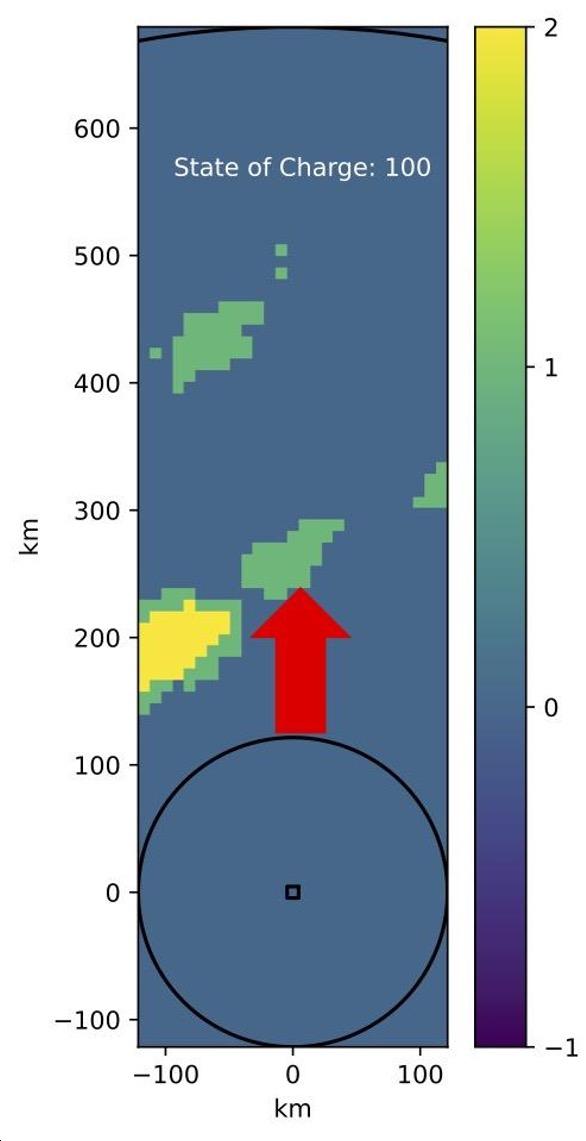
b) Saved energy is used to collect high-value measurements when they are within the primary instrument’s reach
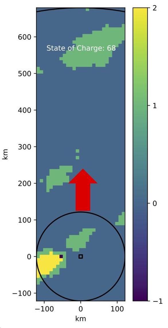
jpl.nasa.gov 35
Dynamic Targeting: Algorithms
jpl.nasa.gov 36
1) Random
2) Greedy Nadir
3) Greedy Lateral
4) Greedy Radar
5) Greedy Window
6) Dynamic Programming
Algorithms: Random
• Representative of most targeting methods on current Earth Science satellites
• It randomly targets the point under nadir 20% of the time to ensure that it meets energy requirements
• It is indifferent to the clouds it is flying over and will most likely miss many high -value targets
• It provides a lower bound on performance
jpl.nasa.gov 37
Algorithms: Greedy Nadir, Lateral, Radar
• They collect observations based on the:
• Current state of charge (SOC)
• Radar reachability window
• Larger reachability window for analysis and sampling
Greedy Nadir Greedy Lateral Greedy Radar
jpl.nasa.gov 38
Algorithms: Greedy Window
• Improves upon greedy radar
• It collects observations based on the:
• Current state of charge (SOC)
• Radar reachability
• Radiometer range
• It accounts for future clouds along the radar’s path
jpl.nasa.gov 39
Algorithms: Dynamic Programming
• Optimal algorithm
• Omniscient, full lookahead
• Requires unrealistic computational and instrument resources
• Cannot be deployed on flight missions
• But useful for this study as it provides an upper bound on performance
jpl.nasa.gov 40
Algorithms: Dynamic Programming Formulation
Assumptions:
• Discrete environment: locations, state of charge, actions
• Finite path length
• Additive, independent rewards
• Rewards among classes differ significantly (by several orders of magnitude) to avoid trade-offs among cloud categories
• E.g: cloud = 1, mid-cloud = 10,000, clear sky = 100,000,000
Markov Decision Process Formulation
• State space = [Location (row), SOC (0-100)]
• Action space = # points inside the radar + don’t sample option
jpl.nasa.gov 41
Algorithms: Insights from the Optimal Solution
• Useful lessons were learned from the DP algorithm
• The optimal policy prioritizes saving energy for rare, high -value targets by:
• Performing atmospheric profiling (i.e., sample low-reward clouds) only when SOC = 100%
• Periodically sampling mid-reward clouds (e.g., rainy anvil, mid-cloud), 1 in every n opportunities
• We incorporate these notions into the Greedy algorithms to improve their science return

jpl.nasa.gov 42
Experiments and Results
jpl.nasa.gov 43
Experimental Setting
4 datasets/scenarios
• SMICES tropical (small): storms, 15 km/pixel
• SMICES non-tropical (large): storms, 15 km/pixel
• GPM/IMERG: global, storms, 4 km/pixel
• MODIS: global, cloud avoidance, ~11 km/pixel
Studies
1. Science return (cloud observations)
2. Lookahead sensitivity analysis
3. Runtimes on flight processors
jpl.nasa.gov 44
Results: SMICES Cloud Observations
● Lookahead = 420 km (SMICES concept), sample 1 in 2 RAs
● Random < G. Nadir < G. Lateral < G. Radar < G. Window < DP
jpl.nasa.gov
45
Random Greedy Nadir Greedy Lateral Greedy Radar Greedy Window DP No sample 80.04 % 79.82 % 79.80 % 80.00 % 80.00 % 78.59 % CS 5.63 % 7.90 % 0.07 % 0.00 % 0.00 % 0.00 % TAC 2.34 % 3.00 % 0.00 % 0.00 % 0.00 % 0.00 % TA 4.25 % 0.11 % 0.01 % 0.00 % 0.00 % 0.00 % RA 7.25 % 18.72 % 18.17% 17.52 % 15.50 % 13.45 % CC 0.18 % 0.25 % 1.95 % 2.69 % 4.70 % 7.96% Random Greedy Nadir Greedy Lateral Greedy Radar Greedy Window DP No sample 80.37 % 80.00 % 80.00 % 80.00 % 80.09 % 80.01 % CS 11.93 % 11.01 % 10.59 % 10.26 % 10.19 % 8.28 % TAC 1.98 % 1.77 % 1.68 % 1.61 % 1.59 % 1.78 % TA 1.94 % 0.80 % 0.62 % 0.56 % 0.55 % 2.17 % RA 2.48 % 4.13 % 4.23 % 4.07 % 3.48 % 2.87 % CC 1.30 % 2.29 % 2.89 % 3.51 % 4.09 % 4.88 %
(U.S. East Coast):
Non-Tropical
fewer storms Tropical (Caribbean): more storms
Results: Global Cloud Observations
● Lookahead = 420 km (SMICES concept), sample 1 in 2 RAs
● Random < G. Nadir < G. Lateral < G. Radar < G. Window < DP
GPM / IMERG: Storm Hunting
MODIS: Cloud Avoidance
46
jpl.nasa.gov
Random Greedy Nadir Greedy Lateral Greedy Radar Greedy Window DP No sample 80.12 % 79.99 % 79.96 % 79.94 % 79.97 % 79.92 % No Storm 19.02 % 16.78 % 12.46 % 10.50 % 10.48 % 10.45 % Rainy Anvil 0.84 % 3.17 % 7.27 % 8.95 % 8.56 % 8.15 % Conv. Core 0.01 % 0.04 % 0.31 % 0.59 % 0.97 % 1.46 % Random Greedy Nadir Greedy Lateral Greedy Radar Greedy Window DP No sample 80.52 % 80.00 % 80.00 % 80.00 % 80.00 % 79.91 % Clouds 12.93 % 11.20 % 10.35 % 9.81 % 9.83 % 9.73 % MidClouds 5.55 % 7.66 % 8.06 % 8.07 % 7.57 % 7.08 % Clear Skies 0.99 % 1.14 % 1.59 % 2.12 % 2.61 % 3.28 %
Results: Science Return Summary
Greedy Window vs. lower/upper bounds
highest value targets: CC, clear skies

● DT substantially collects more high -value targets than baseline (random)
● DT performs relatively close to optimal (DP)
● GPM / IMERG is the most challenging scenario as CC clouds are very rare around the globe
47
jpl.nasa.gov
Scenario/Dataset Baseline Optimal SMICES Tropical (storms) 22.65 0.74 SMICES Non Tropical (storms) 3.19 0.84 GPM / IMERG (global storms) 88.45 0.69 MODIS (global clear skies) 2.63 0.79
Results: Lookahead Sensitivity Analysis (Global Studies)
Greedy Window: trade-off between high and mid-reward targets
high-reward (CC, clear sky)
Farther lookahead:
- closer to optimal
- reduced need to periodically sample mid-reward clouds
* Similar results for SMICES
mid-reward (RA, mid-cloud)
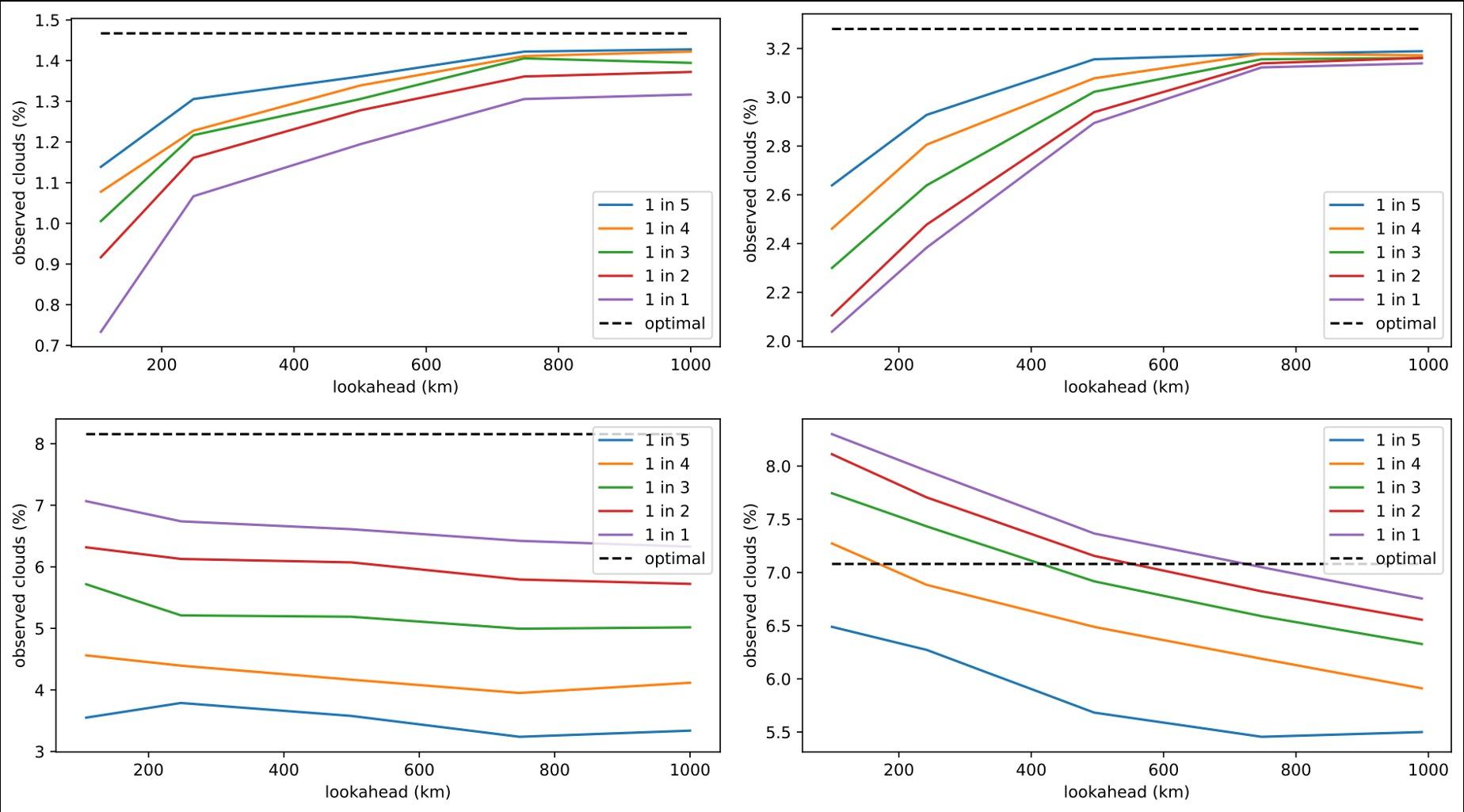
jpl.nasa.gov 48
/ IMERG MODIS
GPM
Results: Runtimes on Flight Processors
● Benchmarking of DT on different flight processors
● Greedy Window algorithm coded in C
● CPU single thread
*MacBook Pro 16’: Intel i9 2.3 GHx octacore processor, 32 GB RAM
49
jpl.nasa.gov
MacBook Pro 16* SBC -2:
Spaceborne Computer-2 Qualcomm Snapdragon 855 GR740/ Sabertooth RAD750 Average Runtime (ms/timestep) ~0.1 ~0.4 ~20 ~1,500 ~2,800
HPE
Conclusions and Future Work
jpl.nasa.gov 50
Ongoing and Future Work
• Customized policies for regions, seasons
• Explore deep reinforcement learning for DT policies ( Breitfeld et al. …)
• Study of pointing with costs use cases (current cases assume electronic steering) [Kangaslahti et al. ICRA 2024]
• Elaboration of instrument reconfiguration use cases (as opposed to pointing)
• Additional studies/ data sets for further evaluation; Planetary Boundary Layer [Candela et al. IGARSS 2024]
• Expansion of use cases to incorporate primary sensor data such as tracking comet and volcanic plumes and to “stare” use cases.
jpl.nasa.gov 51
Closing Remarks
• Dynamic targeting algorithms use lookahead sensor information to improve primary sensor science yield including global (energy, thermal) constraints
• Interpretation of lookahead (ML and other) can present challenges – more work is needed; minority classes, asymmetric loss function
• Presented new optimal DP approach, useful for evaluation purposes
• Evaluated on 4 different datasets/scenarios: storm hunting and cloud avoidance
• DT methods’ performance is much better than baseline (random), close to optimal
• Greater lookahead improves performance
• DT algorithms are extremely fast and produce results approaching optimal
jpl.nasa.gov 52
Acknowledgements
• Alberto Candela, Jason Swope Juan Delfa , Itai Zilberstein, Akseli Kangaslahti, Qing Yue, Marcin Kurowski and the rest of the DT Team
• SMICES Team
• Global storm study: Hui Su, Peyman Tavallali
• This work was supported by the NASA Earth Science and Technology Office (ESTO)
jpl.nasa.gov 53

jpl.nasa.gov 54