
Bayesian system reliability and availability analysis underthe vague environment based on Exponential distribution
RaminGholizadeh1 , Aliakbar M. Shirazi2and
Maghdoode Hadian31Young Researchers Club, Ayatollah Amoli Branch, Islamic Azad University, Amol , Iran.
2Islamic Azad University, Ayatollah Amoli Branch, Mathematic Department,Iran.
3Young Researchers Club, Mashhad Branch, Islamic Azad University, Mashhad,Iran Islamic Azad University, Iran
Abstract
Reliability modeling is the most important discipline of reliable engineering. The main purpose of this paper is to provide a methodology for discussing the vague environment. Actually we discuss on Bayesian system reliability and availability analysis on the vague environment based on Exponential distribution under squared error symmetric and precautionary asymmetric loss functions. In order to apply the Bayesian approach, model parameters are assumed to be vague random variables with vague prior distributions. This approach will be used to create the vague Bayes estimate of system reliability and availability by introducing and applying a theorem called “Resolution Identity” for vague sets. For this purpose, the original problem is transformed into a nonlinear programming problem which is then divided up into eight subproblems to simplify computations. Finally, the results obtained for the subproblems can be used to determine the membership functions of the vague Bayes estimate of system reliability. Finally, the sub problems can be solved by using any commercial optimizers, e.g. GAMS or LINGO.
Keywords: Bayes point estimators, Vague environment, Nonlinear programming; System reliability, System availability, Exponential distribution, Precautionary loss function.
1. Introduction
In the real world there are vaguely specified data values in many applications, such as sensor information. Fuzzy set theory has been proposed to handle such vagueness by generalizing the notion of membership in a set. Essentially, in a fuzzy set each element is associated with a pointvalue selected from the unit interval [0,1], which is termed the grade of membership in the set. A vague set, as well as an Intuitionistic fuzzy set, is a further generalization of a fuzzy set. Instead of using point-based membership as in fuzzy sets, interval-based membership isused in a vague set.Gau and Buehrer (1993) define vague sets. These sets are used by Shyi-Ming Chen and JiannMean Tan (1994). Once the vague (intuitionistic fuzzy) set theory have been introduced, a number of authors investigated the reliability analysis in vague environments. Chen (2003) presented a method to analyze system reliability using the vague set theory, where the reliabilities of system components are represented by vague sets. Kumar et al. (2006) developed a method for
1 - Ramin.gholizadh@gmail.com
2 - Zayrsil@gmail.com
International Journal on Soft Computing ( IJSC ) Vol.3, No.1, February 2012
analyzing system reliability by using interval-valued vague sets, and applied it for the reliability analysis of a Marine Power Plant.
Complex systems may have both kinds of uncertainty. Researchers have stated that probability theory can be used in concert with fuzzy set theory for the modeling ofcomplex systems Zadeh (1995), Barrett and Woodall (1997), Ross, Booker, and Parkinson (2003), and Singpurwalla and Booker (2004). Bayesian statistics provide a natural framework combining random and nonrandom uncertainty so fuzzy Bayesian methods are developed for the solutions of the reliability problems. Sellers and Singpurwalla (2008) addressed the reliability of multistate systems with imprecise state classification. On the other hand, Gholizadeh, Shirazi, Gildeh, and Deiri (2010), Gholizadeh, Shirazi, and Gildeh (2010), Görkemli and Ulusoy (2010), Huang, Zuo, and Sun (2006), Taheri and Zarei (2011), Viertl (2009), and Wu (2004, 2006) addressed the problem of imprecise data (approximately recorded failure time durations and number of failures) in reliability studies.
Fuzzy Bayesian reliability method developed by Wu (2004, 2006).Taheri and Zarei (2011) modeled and evaluated Bayesian system reliability considering the vague environment. Our modeling approach is a generalization of Wu (2004, 2006) and Taheri and Zarei (2011).

Vague environment is introduced in Section 2. Vague point estimator is represented in Section 3. In Section 4, the reliability and availability analysis via vague Bayesian method under squared error and precautionary loss functions for series system, parallel system and k-out-of-n system have been discussed is illustrated on an example. The computational procedures and examples are provided in order to clarify the theory discussed in this paper, and to give a possible insight for applying the vague set to Bayesian system reliability and availability. Conclusions and future extensions of this work are given in Section 6.
2. Vague environment
Definition 1.A vague set in a universe of discourse is characterized by a true membership function, , and a false membership function, , as follows: ∶ →[0,1], ∶ →[0,1], and ( )+ ( )≤1, where ( ) is a lower bound on the grade of membership of derived from the evidence for , and ) is a lower bound on the grade of membership of the negation of derived from the evidence against .
Suppose { , , . A vague set of the universe of discourse can be represented by = ∑ ( ),1 )]/ , where 0≤ ( )≤1 ( )≤1 and 1 ≤ ≤ . In other words, the grade of membership of is bounded to a subinterval [ ( ),1 )of [0, 1]. Thus, vague sets are a generalization of Fuzzy sets, since the grade of membership ( ) of in Definition 1 may be inexact in a vague set. We now depict a vague set in Fig. 1.


Definition 2.The complement of a vague set is denoted by and is defined by
Definition 3.A vague set is contained in another vague set , ⊆ , if and only if, ( )≤ ( ),
Definition 4.Two vague sets and are equal, written as = , if and only if, ⊆ and ⊆ ; that is ( )=


Definition 5.Let be a vague set of . Then, we define -cuts and -cuts of as the crisp sets of given by
Definition 6.Let be a vague set of ⊆ . We say that is convex if for all , ∈ and in [0,1],
Definition 7.A vague set of with continuous membership functions and is called a vague number if and only if and , for all , ∈(0,1], are bounded closed intervals; i.e.


We denote the class of all vague numbers by ( )
Definition 8.Thevague number is called a triangular vague number, if
International Journal on Soft Computing ( IJSC ) Vol.3, No.1, February 2012
Where ∈[1,∞). We denote such a vague number by =( , , , )
Proposition 1.(Taheri and Zarei (2011); Resolution Identity for Vague Sets) Let be a vague set of . Then
( )= sup ∈[ , ] ( ), 0≤ ≤1,
( )= sup ∈[ , ] ( ), 0≤ ≤1,


Where, (.) is denoted for the indicator function.
3. Vague point estimator
With according to Taheri and Zarei (2011), Let X ).be a vague valued function. Then, is called to be a vague random variable if and for all 0≤α ,α ≤1, are (ordinary) random variables. Too, Let be a vague random variable whose distribution depends on a vague parameter . So, it could be said that distributions of (crisp) random variables estimate based on a Bayes approach. According to this approach, random variable so that the crisp random variables with parameters ( ) ,…,( ) ,( ) respectively.

Concerning Definition 7, we can find the Bayes point estimator for each ∈ , Consider
Then, contains all of the Bayes point estimators for each ∈ , . The same argument can be established for ∈


The vague Bayes point estimator for the vague parameter is defined to be a vague number , where )

( ( )= sup ∈[ , ] ( ), 0≤ ≤1, )
( ( )= sup ∈[ , ] . ( ), 0≤ ≤1,
4. Vague Bayesian system reliability and availability
In the Bayesian approach to system reliability, some prior distributions are assigned to the components of the system. Then, the posterior distribution of each component’s reliability can be found using the Bayes theorem. We can derive, therefore, the posterior distribution of the system reliability from the posterior distribution of each component reliability. The key point in this approach is that system reliability can be expressed as a product of independentrandom variables which corresponds to either component reliability (for series system) or to component unreliability (for parallel systems). To this end, we need to use the method of Mellin integral transform [2] described below.
4.1 Mellin transformation
Definition 9. [2] Let be a non-negative random variable with pdf ( ). The Mellin transform of ,with respect to the complex parameter, is defined by ( ; ) =∫ ( ) ( ) (4)
Such a transform exists if ∫ | ( )| ( )is bounded for some >0

Remark1. Based on the above definition, the inverse Mellin transform of ( ; ) is given by ( )= ( , ) , where + ∞ are complex values [2].


Remark 2. It is convenient to regard the Mellin transform as the moments of , i.e. ( ; ) = ( )
Theorem 1. [25] Let , be independent random variables with ’s , , respectively. Let ( ) be the of the random variable =∏ . Then
; ) =∏ ( ; ) (5)
With the help of Theorem1, we can obtain the posterior distribution of the system reliability from the posterior distribution of the component reliabilities. On the other hand, the Bayes estimator of the system reliability, under the squared error loss function, is the mean of the posterior distribution [21], so that we can use Eq. (4), for = 2, to obtain the Bayes estimator of the system reliability.
4.2 Bayesian approach to system reliability
The fuzzy Bayesian interval estimate of reliability is calculated using the method proposed by Wu (2006). Let random variable be the th failure time of the th componentsand be the realization of this random variable, = 1,2, , , = 1,2, , . It is assumed that , = 1,2, , , are independent and identically distributed exponential random variables with parameter . is unknown; therefore, a gamma distribution with parameters and is assigned as prior distribution to quantify the uncertainty in . From previous experience we know the parameters of the prior distribution and .They can be interpreted as numbers of failures that occur in the duration for component since the expected value of gammadistribution is ⁄ . On the total operating time of , =∑ failures are observed for the component . Since the gamma distribution is a conjugate prior distribution for the exponential sampling distribution, the posterior distribution of is a gamma distribution with parameters +m)and ( + ). Reliability of the components for the duration ∗ is ( ∗)= and it is monotonically decreasing function of , so there is aone-to-one relationship between and . Therefore the unique inverse is λ = lnr t∗ ⁄ so the distribution of can be determined fromthedistribution of as ( )=
Where ( ) is either prior or posterior distribution of is corresponding prior or posterior distribution of (Martz and Waller,1991). Assigning a gamma ( , ) prior distribution to corresponds to assigning a Negative-Log-Gamma ( , t∗ ⁄ ) priordistribution
International Journal on Soft Computing ( IJSC ) Vol.3, No.1, February 2012
. Given the data, the posterior distribution of is a Negative-Log-Gamma ( + ( + ) ∗ ⁄ ) distribution.

Series system
Consider a series system consisting of independent components. The system reliability is =∏ .So from Eq. (5), the Mellin transform of the ( | , )of system reliability is given by [ ( | , ); ]=∏ ) (6)


Under a squared error loss function, the Bayes point estimate of the system reliability r isgiven as ]= [ ( | , ); =2]=∏ (7)

The Bayes point estimate of the system reliability under a precautionary loss function is: , ]) =( [ ( | , ); =3]) =∏ (8)
Now, suppose in a complex system the number of failures and failure times may be recorded imprecisely due to equipment and human errors. For such cases this imprecision also should be quantified in the calculations. Here vague set theory is used to quantify the uncertainty of imprecision. Failure rate, λ, reliability,r, and failure times,t , are taken as vague random variables. It is assumed that prior distribution parameters are known from the previous experience so those and are taken as vague number (the parameter θ can be interpreted as the ‘pseudo’ number of and failures in a lifetime test of durationθ ‘pseudo’ time units) the Bayes point estimates of( ) , ( ) , ( ) and ( ) under a squared error loss function are given by ) =∏ ) , ) =∏ ) (9) +
( ) , 10)
the Bayes point estimates of under a precautionary loss function are given by
Respectively, for all [ ]0,1 ∈ . According to the discussions in Section 3, let
The above intervals contain all of the Bayes estimators for each ∈ , . The same intervals can be established for ∈ . But, for


have
Therefore, and can be rewritten as
Now, using Proposition 1, the truth membership function and the false membership function of the vague Bayes estimate of , denoted by , are defined as follows
Parallel systems
For a parallel system consisting of independent components, the system reliability is =1
∏ (1 )where is the component reliability of the th component. Equivalently, the ystemunreliability is the product of component unreliabilities = 1 , i.e., =


.The Bayes point estimate of system unreliability is given by
The Bayes point estimate of the system reliability r under a squared error loss function is given by


The Bayes point estimate of the system reliability r under a precautionary loss function is given by
Under the vague assumptions as described above, the Bayes point estimates of under a precautionary loss function are given by


Respectively, for all α∈[0,1] the membership function of the vague Bayes point estimate of system reliability r is defined by the same way as discussed above.
k-out-of-m system
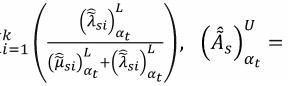
For a k-out-of-m system consisting of m independent and identical components, the system reliability is given by
That is the reliability of the (common) component. The Bayes point estimate of system reliability r is the mean E[R| , ] under the squared error loss function, and is given by

The Bayes point estimate of system reliability at time , under a squared loss function, given by ,

Under the vague assumptions as described above, the Bayes point estimates of ( ) , ( ) , ( ) and( ) under a squared error loss function are given by ( 1)


Under the vague assumptions as described above, the Bayes point estimates of under a precautionary loss function are given by


Respectively, for all α∈[0,1] the membership function of the vague Bayes point estimate of system reliability is defined by the same way as discussed above


4.3 Bayesian approach to system availability
Martz and Waller, (1991) presented the method to calculate the availability of a repairable system
That X is the failure time and Y is the repair time. Assume X and Y are independent variables and have exponential distributions with parameters λ and μ respectively. Separate gamma distributions are assigned as prior distributions to λ and μ. To determine the availability of the system, the parameters of exponential distribution should be estimated. Vague Bayesian estimations under the squared error loss function by use Wu (2004) are given by
Vague Bayesian estimations under the precautionary loss function are given by

and are the prior distribution parameters of ; they are assumed to be known from previous experience.For the parameter of repair time distribution, vague Bayes point estimators under the squared error loss function are given in (34) and (35)
Vague Bayesian estimations under the precautionary loss function are given by
and are the prior distribution parameters of ; they are assumed to be known from previous experience.
Vague Bayes point estimators under the squared error loss function of availability interval bounds are given by


Vague Bayes point estimators under the precautionary loss function of availability interval
The availability of a series system consisting of independent components can be calculated with Eq. (42) (Martz and Waller, 1991)


Inserting the vague Bayesian estimates of failure and repair rates into (42), vague Bayesian availability equations of a series system under squared error loss functions are given in (43) and (44) respectively

Vague Bayesian availability equations of a series system under precautionary loss functions are given by
Respectively, for all [ ]0,1 ∈ . According to the discussions in Section 3, let
The above intervals contain all of the Bayes estimators for each ∈ . The same intervals can be established for ∈ . But, for α< have


Therefore, and can be rewritten as =
Now, using Proposition 1, the truth membership function and the false membership function of the vague Bayes estimate of , denoted by are defined as follows


( )= ] ( ), 0≤ ≤1 (49)
( )= ] . ( ), 0≤ ≤1 (50)
The availability of a parallel system consisting of independent components can be calculated with Eqs. (51)– (53) (Martz and Waller, 1991)


In the same way, inserting the vague Bayesian estimates of failure and repair rate into (50), Vague Bayesian availability equations of a parallel system under squared error loss functions are given in (53) and (54) respectively 1
Vague Bayesian availability equations of a parallel system under precautionary loss functions are given by


Respectively, for all α∈[0,1] the membership function of the vague Bayes point estimate of system availability is defined by the same way as discussed above.


For a k-out-of-m system consisting of m independent and identical components, the system availability is given by
=∑ (1 ) (58)
=∑ (59)
Vague Bayesian availability equations of a -out-of- system under squared error loss functions is given by


Vague Bayesian availability equations of a parallel system under precautionary loss functions are given by
4 Computational procedures and example we need to apply some computational techniques for evaluating the truth and false membership degrees of the vague Bayes point estimate as presented in Eq. (2) and Eq. (3) will be provided. From Eq. (1), we adopt the following notations
From Eq. (1), the truth and false membership functions of the vague Bayes estimate are given by
Therefore, needs to be solved the following type of nonlinear programming problem

Let and be the objective values of subproblems and be the objective values of subproblems , respectively. Assume that, = , , , and = and be the objective values of the original problems with optimal solution respectively (in fact = , = ). In according to Wu (2004), we have ∗ = and = , so to obtain the objective value and of the original nonlinear programming problems, it will be enough to just solve the eight sub-problems and .


The follow data show that the failure times and repair times are assumed as vague numbers, since the failure times and repair times cannot be recorded precisely due to human errors, machine errors, or some unexpected situations. The simulated failure times and repair times are presented in Table 1 For example component 1, the first failure time and repair time are around 20 and 15 h, respectively the second failure time and repair time are around30 and 20h. There are the same explanations for components 2 and 3. The prior distribution parameters (pseudo) of the failure rate and repair rate are presented in Table 2.

Where 3 , 4 , 5, 6 , 8,10 , 15 , 20, 25, 30, 35, 45and50are vague numbers with the following membership functions
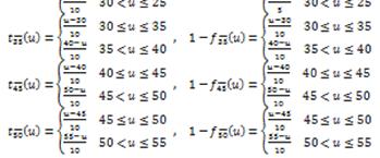


Now, we want to obtain the vague Bayesian system reliability and availability. First of all, note that the cuts and -cuts of the vague numbers3 ,4, 5, 6 , 8,10 , 15 , 20, 25, 30 , 35, 45and50 are


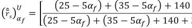
The vague Bayes point estimates of reliability under different loss functions of , , and are obtained as follows (for all , ∈[0,1])


The vague Bayes point estimates of availability under different loss functions of are obtained as follows (for all , ∈[0,1])


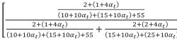


Therefore, we just need to solve subproblems .We use the method provided in Section 5 to solve these problems. For =0.5yields


021687= 05. on
the other hand, α =1 yields 21687= 1 f (0.21687)=1. Since V =[027851,029998], we are just interested in considering the system reliability ∈ . By applying the Supplemental Procedure Wu (2004), we have, for ∈


(i) if < 021687, then we solve the following problem, using a suitable software (LINGO):
(ii) if > 021687, then we solve the following problem:
Therefore we now can obtain the membership degree for any given Bayes point estimate of vague system reliability by evaluating the above formulas.
Above conclusion is defined by the same way for system availability.
6. Conclusion
We developed Bayesian approach to system reliability analysis in the vague environment, Taheri and Zarei (2011), for system availability under different loss function based on Exponential distribution. In order to evaluate the truth and false membership degrees of the vague Bayes estimate, a nonlinear programming problem was solved. The vague Bayesian approach to system reliability and availability is a generalized version of the fuzzy Bayesian reliability and availability, and it is also an extension of the conventional Bayesian system reliability and availability.
For future research, distributions other than exponential distribution can be used for failure and repair times of system. In addition to vague data in the analysis, vague multi state reli- reliability can be considered.
References
[1] Barrett J. D.,& Woodall W. H., A probabilistic alternative to fuzzy logic controllers, IIE Transactions, 29 (1997), 459–467.
[2 ]Chen S. M., Analyzing fuzzy system reliability using vague set theory, International Journal of Applied Science and Engineering, 1 (2003) 82–88.
[3] Chen S. M. and Tan J. M., Handling multicriteria fuzzy decision-making problems based on vague set theory, Fuzzy Sets and Systems, 67 (1994) 163 172.
[4] Gau W.L. and Buehrer D.J., Vague sets, IEEE Trans. Systems Man Cybernet. 23(2) (1993) 610-614.
International Journal on Soft Computing ( IJSC ) Vol.3, No.1, February 2012
[5] Gholizadeh R., Shirazi A. M., Gildeh B. S., &Deiri E., Fuzzy Bayesian system reliability assessment based on Pascal distribution, Structural and Multidisciplinary Optimization, 40 (2010), 467–475.
[6] Gholizadeh R., Shirazi A. M. and Gildeh B. S., Fuzzy Bayesian system reliability assessment based on prior two-parameter exponential distribution under different loss functions. Software Testing, Verification and Reliability, (2010), DOI: 10.1002/stvr.436.
[7] Görkemli L., Ulusoy S. K., Fuzzy Bayesian reliability and availability analysis of production systems, Computers & Industrial Engineering 59 (2010) 690
696.
[8] Huang H., Zuo M. J. & Sun Z., Bayesian reliability analysis for fuzzy lifetime data. Fuzzy Sets and Systems, 157(12) (2006), 1674–1686.
[9] Kumar A., Yadav P.S. and Kumar S., Fuzzy reliability of a marine power plant using interval valued vague sets, International Journal of Applied Science and Engineering, 4 (2006) 71–82.
[10] Martz HF, Waller RA, Bayesian reliability analysis. Wiley, New York (1982).
[11] Ross, T. J., Booker, J. M., & Parkinson, W. J. (2003). Fuzzy logic and probability applications bridging the gap. Philadelphia: ASA-SIAM.
[12] Sellers K. F. &Singpurwalla N. D., Many-valued logic in multistate and vague stochastic systems. International Statistical Review, 76(2) (2008), 247–267.
[13] Singpurwalla N. D. & Booker J. B., Membership functions and probability measures sets. Journal of the American Statistical Association, 99(467) (2004), 867–877.
[14] Springer MD, Thompson WE. The distribution of products of independent random variables. SIAM Journal on Applied Mathematics 1966; 14:511–526.
[15] Taheri S. M., Zarei R., Bayesian system reliability assessment under the vague environment, Applied Soft Computing, 11 (2011) 1614–1622.
[16] Viertl R., On reliability estimation based on fuzzy lifetime data. Journal of Statistical Planning And Inference, 139 (2009), 1750–1755.
[17] Wu H.C., Fuzzy reliability estimation using Bayesian approach, Computers & Industrial Engineering 46 (2004) 476–493.
[18] Wu H.C., Bayesian system reliability assessment under fuzzy environments, Reliability Engineering and System Safety 83 (2004) 277–286.
[19] Wu H.C., Fuzzy Bayesian system reliability assessment based on exponential distribution, Applied Mathematical Modeling 30 (2006) 509–530.
[20] Zadeh L. A., Discussion: Probability theory and fuzzy logic are complementary rather than competitive. Technoetrics, 37(3) (1995), 271–276.