The Effectiveness of a Vehicle Manufacturing Line Using Probabilistic Process Timing

ISSN: 2321 9653; IC Value: 45.98; SJ Impact Factor: 7.538

Volume 10 Issue XI Nov 2022 Available at www.ijraset.com

The Effectiveness of a Vehicle Manufacturing Line Using Probabilistic Process Timing

Yogesh Ahlawat Deenbandhu Chhoturam University of Science and Technology, Murthal, Sonipat 131039, India

Abstract: Automotive manufacturing involves several steps, starting with the casting of components and moving on to the machining and assembly processes. The assembly system, particularly for the Single Cylinder S.I. Engine, will be the only emphasis of this project. A considerable number of components must be integrated throughout the engine assembly process. The creation of a decision assistance system based on a discrete event simulation model is discussed in the work provided in this paper. The four closed loop network arrangement of vehicle assembly and preassembly lines connected by conveyors is targeted at a particular type of manufacturing lines. The design and execution of such industrial processes frequently include simulation. This simulation research aims to select the process throughput for the Single Cylinder S.I. Engine Assembly line. Any possible machine bottlenecks will be identified by the simulation study to avoid blockages and starvation and increase process throughput. Machine cycle times for various processes should be included in the input data for the research. The Arena simulation program will be utilized in this investigation. The goal is to use existing equipment to boost output on the present Head Assembly Line and Sub-Assembly Lines to an anticipated capacity. The outcomes of the simulation will be used to pinpoint the assembly line procedures that may have an impact on the S.I. Engine's manufacturing schedule. By contrast the study's findings with the actual process throughput, the findings will be illustrated. Additionally, statistical analysis will be done to boost performance.

Keywords: Automobile industry, Assembly lines, Conveyors, Closed loops, Discrete event simulation.

I. INTRODUCTION

Simulating interactions between a complex system's subsystems in a computer model is one of the most valuable ways for predicting a complex system's dynamic performance [1]. Simulation modeling may be defined as the process of building a model that represents a real system and utilizing that model to conduct experiments to better understand its behavior and assess the effects of potential operational changes [2 5]. When a system performs admirably in a predetermined amount of time and under predetermined circumstances, it is said to be reliable [15]. In other words, reliability is the likelihood that, under typical operating conditions, a system will perform as intended, without any failure, for a predetermined amount of time [16]. Having a dependable operation is one of the biggest issues confronting the deployment of industry 4.0 due to the complexity of systems and the automation of industrial systems rising [13,14]. Asset performance analysis, such as reliability indices, is required to establish a reliable working condition coupled with high productivity and quality in order to maintain competitiveness in the global market [18,20]. Additionally, it's important to shorten the time spent studying simulation findings. Therefore, the adoption of discrete event simulation (DES) as a tool for choosing improvement projects in operating manufacturing systems can significantly increase with the development of new work methods regarding flow simulation that aim to shorten the analysis phase and also integrate the decision makers into this process [7].

In the project report, a software solution to a business issue is presented. Here, the simulation was carried out using the ARENA program A computer simulation study on the Automotive Manufacturing System's Engine Assembly line is the first step in the procedure. Engine parts are assembled on machines in the Engine Assembly lines, which then transfer the engine pieces on pallets with the use of conveyors. The interplay of many resources, processes, and products results in a variety of potential outcomes that cannot be assessed without a simulation approach.

Experimenting via trial and error with a real system is costly and useless. Therefore, using a simulation modelling approach makes it possible to do a what if analysis study of the existing system without interfering with the actual instance. The use of a decision supporting tool is necessary in order to save time. Common application goals for simulation in the automotive/manufacturing sector were proposed by Jayaraman and Agarwal in 1996 [9]. These included determining system throughput, identifying bottlenecks, optimizing staff allocation and use, contrasting operational philosophies, analyzing materials storage problems, designing materials handling systems, and designing logistics systems.

ISSN: 2321 9653; IC Value: 45.98; SJ Impact Factor: 7.538 Volume 10 Issue XI Nov 2022 Available at www.ijraset.com

The throughput of assembly lines, which takes into account work in progress (WIP), bottlenecks, and machine cycle durations, is generally used to quantify them. Through a model simulation with Arena Software, the report identifies the input data, including machine cycle time distributions. This model illustrates the workflow. The simulation results from Arena look at the many components needed for a good system. The outcomes will highlight the numerous obstacles; therefore, it is helpful to consider how to work efficiency may be increased.

The production line's behavior evolves as time passes. The necessity to modify the current line and make it flexible enough to adapt to the forthcoming approaching spontaneous modifications, as necessary, grows as the demand or requirement of the technology changes in this expanding planet. A powerful tool for comprehending complex systems and making decisions under a variety of circumstances, including conflict, risk management, and both certainty and ambiguity Manufacturing is essential to both emerging and established nations' economic development. Emerging nations like India have increased their attention on the manufacturing industry as a strategy for progress.

To further emphasize the importance of the manufacturing industry, the Indian government has introduced the "Make in India" campaign. Therefore, when the manufacturing sector grows, businesses and industrial facilities will unintentionally follow the road of optimization. This makes it difficult for production managers to make the most use of the available resources. Since systems are becoming more sophisticated, making judgments on a range of issues on the shop floor can be challenging. Analytical analysis of the issues is challenging due to the interactive nature of the effective components in such a complex production logistics system, such as stochastic characteristics, such as process delays, market demand, and resource failure [10].

The project's goal is to assess machine cycle durations to find any possible bottlenecks and eliminate assembly line hunger and blockages to increase process throughput. The following are the project's goals:

1) Determination of the assembly line system's process throughput.

2) The abandonment of static instruments with known deterministic parameters and dynamics.

3) Increasing quality everywhere

4) Find bottlenecks, whether they are mechanical or due to another factor.

5) Progress is being made on the system.

6) Making choices for impromptu employment.

7) To investigate the many adjustments that are currently accessible.

8) The duration of a machine cycle at any system station.

9) Space optimization is necessary.

II. LITERATURE REVIEW

An assembly that may be "easily" removed and changed in order to recover engine performance lost to wear or engine failure is referred to as an "engine assembly." The cylinder liners, pistons, piston rings, and connecting rods of heavy duty engines used in industrial applications may all be changed as needed during an overhaul without having to remove the entire engine unit from its installation. The engine may be restored to its genuine new engine performance using this technique, which also boosts engine value and decreases downtime.

Simulating interactions between a complex system's subsystems in a computer model is one of the most valuable ways for predicting a complex system's dynamic performance [1]. To predict the performance characteristics of a closed loop manufacturing line that is characterized by low capacity buffers and prone to failure, Douard and Baynat [19] devised an analytical model. Spreadsheets and other static methods cannot be used to solve many line design problems because of all the dynamics involved and the non deterministic nature of the parameters. The manufacturing system parameter is supported by built in constructions in discrete event simulation tools that are currently available. The capacity to mimic unpredictable downtime events, varied cycle durations and unpredictable repair times is a feature of every simulation software. Discrete event simulation is also extremely helpful in analyzing various options based on various parameter values. The essential parameters may be changed to do a sensitivity analysis for each option [12].

Several research articles on a simulation that used ARENA to model and optimize real time processes were cited. Even if the optimization parameter varies from study to study, the fundamental nature of the research never changes. These studies have provided answers to the corresponding challenges by utilizing ARENA simulation capabilities. The study's objectives were to reduce flow time, enhance the layout, and increase output [11]. After analyzing the input data using the ARENA Input Analyzer module, the manufacturing process has been modeled, and flow logic has been developed in accordance with the current process flow.

ISSN: 2321 9653; IC Value: 45.98; SJ Impact Factor: 7.538 Volume 10 Issue XI Nov 2022 Available at www.ijraset.com

The authors have identified the process bottlenecks based on the simulation reports produced, and as a result, modifications have been proposed, mostly in relation to the process structure and the manpower allotted. The industry used an antiquated method of production planning, wherein the task is handled by a single person or a small group of individuals. This resulted in operational issues including ineffective staffing levels, resource underutilization, bottlenecks, and mayhem if human judgment failed. In the research, the traditional method of planning production backward is highlighted and examined. There doesn't seem to be much information in the literature, particularly in academic journals, dealing with the study of actual closed loop production lines using discrete event simulation, with the exception of Ladbrook et al. presentation of a simulation study of the camshaft machining line at Ford Valencia. When the goal of the research is the creation of analytical models for these kinds of arrangements, there is a greater choice of literature and standard textbooks available [6]

At VCT, the bottleneck analysis performed using DES now uses either the utilization detection approach or the average waiting for time detection method [7]. The average waiting time detection technique determines how long it usually takes for a workpiece to reach a station for processing. Bottleneck stations are those where workpieces queue up for the longest periods of time. The percentage of time a station is in its active condition is measured using the utilization technique. As a result, the bottleneck station is the one with the highest active %. According to Roser, Nakano, and Tanaka (2001) [8], the utilization approach should take the working and repair percentages into account because both working hours and repair periods can put a load on the system. As used actively, this is this. According to Jayaraman and Gunal (1997), who spoke specifically about the automotive industry, DES is now a common tool used in the design and implementation of various automotive manufacturing systems, from a connecting rod machining sub system to the much more complex automotive assembly systems [12].

In fixed applications, the engine assembly is normally serviced on site due to its size, weight, and the difficulties involved in removing and transporting them for repair. Instead of doing so out of a desire to improve engine serviceability, the engine must be designed for "simple" service. The need for advancement in both professional and educational terms has led to the development of the simulation approach. Simulation modelling and analysis are required to address the current issues and challenges on the path to advancing technology and progress in every area where people are in need.

The history of simulation in steps

1) The 1940s As part of the Manhattan Project to research neutron scattering, mathematicians John von Neumann and Stanislaw Ulan created the first simulation technique known as "Monte Carlo."

2) The first specialized simulation language, SIMSCRIPT, was created in the 1960s by Harry Markowitz at the RAND Corporation.

3) The 1970s saw the beginning of study into the mathematical underpinnings of simulation.

4) The 1980s saw the development of graphical user interfaces, object oriented programming, and computation based simulation software.

5) The 1990s saw the development of simulation based optimization techniques and web based simulation.

The emphasis now being placed on simulation software development is on the automation of the modeling process. Some methods offer a means of locating the issue so that a computer program may be created automatically. For a specific class of modeling problems that can be submitted as data to the system, other systems offer a general framework. Simulations of flexible manufacturing systems are an example of the latter. The majority of modern advancements use color graphics in some capacity. Better user interfaces, more power, and more affordable computer hardware and software are on the horizon. The main advantage is that customers are becoming more involved in the modeling process. This report provides a summary of these advancements as well as suggestions for the future.

III. METHODOLOGY

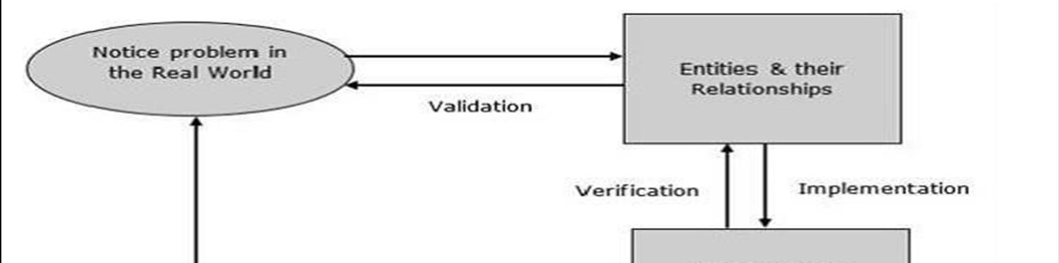
This stage will specify the model's performance requirements or the qualities that the conceptual model must possess in order to accurately represent the real system. Finding the essential elements of the current real system is the first step. Then, provide the facts needed to help create a conceptual model by using a decision analytic framework to determine the crucial decisions. The criteria for developing and subsequently evaluating the model's utility are put into use. Validating the model is the challenge that simulation modeling analysis encounters. The simulation model is only valid if it accurately represents the real system; otherwise, it is useless.

ISSN: 2321 9653; IC Value: 45.98; SJ Impact Factor: 7.538

Volume 10 Issue XI Nov 2022 Available at www.ijraset.com

The two processes in any simulation project to validate a model are validation and verification.

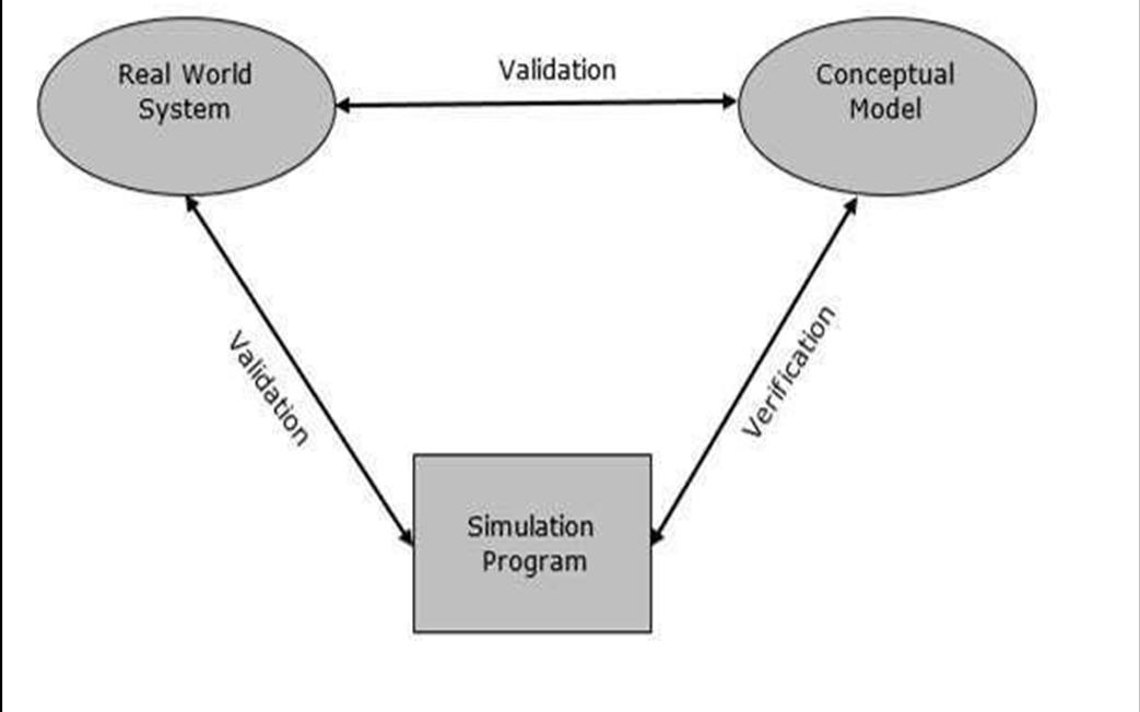
1) Validation is the process of comparing two conceptual model findings to the actual system. If the comparison is accurate, it is legitimate; otherwise, it is invalid.

2) Verification involves comparing the two outcomes to make sure they are accurate. By contrasting the developer's conceptual description and requirements with the model's implementation and the data it is tied to.

Figure 1 Validation of Model [21]

A simulation is essentially a copy or imitation of reality. In order to understand how a system behaves and functions, simulation modeling is the process of creating a model of the real system via many tests based on various factors. The process of creating a simulation model is circular and connected as shown in Figure 1

A. Software for Simulation modeling: Arena.

System Modelling Corporation created the discrete event simulation based program Arena. It is purchased by Rockwell automation in 2000. Microsoft Windows serves as its operating system. This software uses the simulation language and the SIMAN processor These modules, which take the form of boxes with various forms, represent processes and are linked together by connecter lines that define the flow of entities. Every module performs unique operations in relation to the flow, time, and entities. Reports may be produced using data like WIP (work in process) and cycle time. As it is coupled with Microsoft technologies, including Visual Basic for Applications, further automation of models may also be done if a specific algorithm is required as shown in Figure 2. It also supports the import of Microsoft Visio flowcharts, Access databases, and Excel spreadsheets. It is employed by businesses that simulate commercial operations. Early simulation development takes more time, but speedier installation and product optimization can cut down on project duration overall.

ISSN: 2321 9653; IC Value: 45.98; SJ Impact Factor: 7.538

Volume 10 Issue XI Nov 2022 Available at www.ijraset.com

B. Conceptual framework

Here, the simulation research serves as a means of presenting the simulation's potential applications. To be precise, this is the creation and analysis of several assembly line layouts in a machinery industry using the Arena Simulation environment. In our investigation, an engine assembly system a typical manufacturing part is selected from the business whose process flow is provided.

In terms of science, simulation modeling is the process of creating and testing a digital version of a physical model in order to forecast how it will operate in reality.

The framework for simulation modeling depends on the kind of event that will be the focus, thus the first step is to ascertain the event's nature.

Simulation modeling may be divided into the following categories depending on the nature of the event:

1) Monte Carlo/ Risk Analysis Simulation.

2) Agent Based Modeling & Simulation.

3) Discrete Event Simulation.

4) System Dynamics Simulation Solution.

a) Monte Carlo/ Risk Analysis Simulation: John Von Neumann and Stanislaw Ulam, two mathematicians, created the Monte Carlo Simulation during World War 2. This technique, which was first employed to determine how far neutrons would travel through various materials, quickly gained popularity and found several uses in the commercial sector. It is a method of solving probability issues in mathematics that makes use of random variables. For generating pathways, various simulations are done, and the solution is obtained by applying the appropriate numerical calculations. Both the design of a mathematical model and its experimental experimentation is impractical Physical science, computational biology, statistics, artificial intelligence, and quantitative finance all make extensive use of this simulation technique. It is important to remember that issues in Monte Carlo Simulation have a probabilistic foundation. Repetitive experimentation is used in this strategy to investigate such a situation.

b) Agent Based Modeling & Simulation: A computer model known as an agent based model (ABM) is used to simulate the actions and interactions of autonomous agents to evaluate how those actions and interactions will affect the system as a whole. It focuses on a particular system element. The agent based modeling technique has no restrictions since it directly focuses on a single individual item, its behavior, and its interactions. Because of this, agent based simulation is a suitable management tool. Instead of creating a new agent, agent based modeling focuses on finding explanations for the collective behavior of agents that follow straightforward principles. The simulation produces a fine tuned optimization by offering the most specific and straightforward method to model, predict, and compare diverse scenarios.

c) Discrete Event Simulation: The system changes that take place during this type of simulation are discontinuous. Each event takes place at a certain moment in time and represents a shift in the system's state. As a result, any change that occurs in the system is referred to as an event. Discrete simulation can be used in the following situations: Layout Planning The production system or plant layout is designed in a certain way to make the most use of the available resources. The engine assembly line system follows a similar procedure. On numerous assembly line stations, various production processes are carried out. Capacity Management Determine the manufacturing capacity that a business needs to fulfill shifting consumer demands for its products through capacity planning. Every company plans its capacity to ensure that its resources are used to the fullest extent possible. The engine assembly line follows the same procedure. Performing Manufacturing Systems, the efficient use of resources, the promotion of quality management practices, and the use of procedures to deal with unplanned events all affect how well the manufacturing system performs.

Control and planning for production, in essence, entails creating a framework or organization for the production process as shown in Figure 3. In order to maximize the effectiveness of the engine assembly system for a manufacturing plant, it is also described as the work process to distribute different controls, such as human resources, raw materials, and mechanical operations.

ISSN: 2321 9653; IC Value: 45.98; SJ Impact Factor: 7.538

Volume 10 Issue XI Nov 2022 Available at www.ijraset.com

Figure 3 Steps in Production Planning and Control

C. Developing Simulation Models

System elements, input variables, performance measurements, and functional linkages are all included in simulation models [22].

The steps for creating a simulation model are shown below.

1) Establish the specifications for a prospective system or determine the issue with an existing system

2) Design the issue while considering the constraints and elements of the current system.

3) Gather and begin processing the system's input while keeping an eye on its operation and output.

4) Utilizing network diagrams to build the model and a variety of verification tools to validate it.

5) Validate the model by contrasting it with the actual system's performance in various scenarios.

6) Make a detailed description of the model that contains its goals, underlying assumptions, input parameters, and performance for later use.

7) Choose a suitable experimental strategy in accordance with the needs.

8) Create experimental settings for the model, then track the outcome.

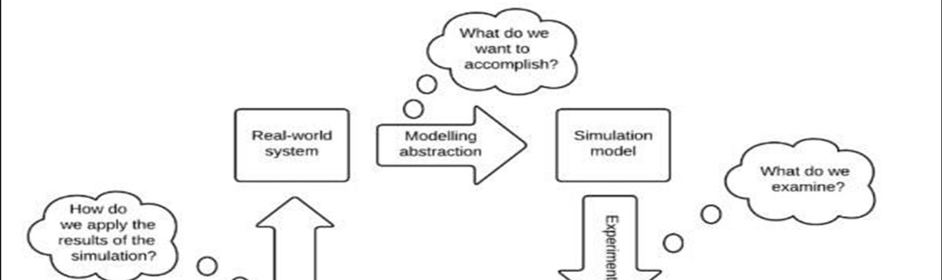
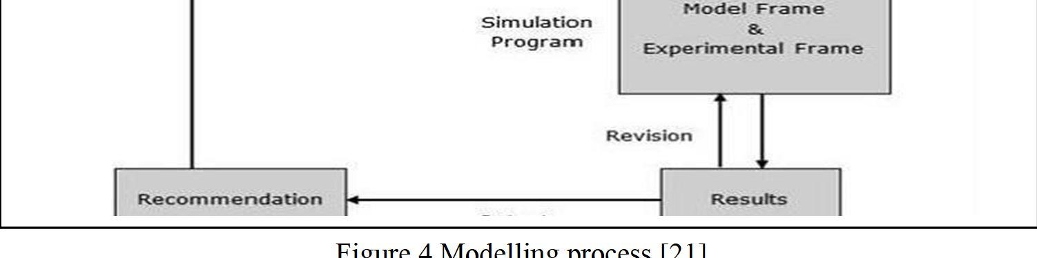
D. Flow diagram for the modeling process: The modeling process includes the following steps as shown in Figure 4:

Figure 4 Modelling process [21]

ISSN: 2321 9653; IC Value: 45.98; SJ Impact Factor: 7.538

Volume 10 Issue XI Nov 2022 Available at www.ijraset.com

Analyzing the issue is an essential step. Understanding the issue fully at this point will help you decide whether to classify it as deterministic or stochastic. to carry out the straightforward actions listed below that assist with model design

1) Gather information based on system behavior and anticipated needs.

2) Analyse the system's attributes, its presumptions, and the steps that must be completed for the model to succeed.

3) Discover the model's variable names, functions, units, connections, and applications.

4) Use an appropriate methodology to solve the model, and then use verification tools to confirm the outcome. Verify the outcome next.

5) Create a report that contains the findings, interpretations, analysis, and recommendations.

After completing all model related processes, offer recommendations. It comprises resources, investment, algorithms, and other tools.

E. Collection of the data from the company

The firm provides complete information on the numerous tasks carried out on the engine assembly line for the Single Cylinder S.I. Engine. Before being removed from the line, all finished engine assemblies are put through testing. Engine assemblies that do not pass the testing are diverted onto a spur and, if feasible, repaired.

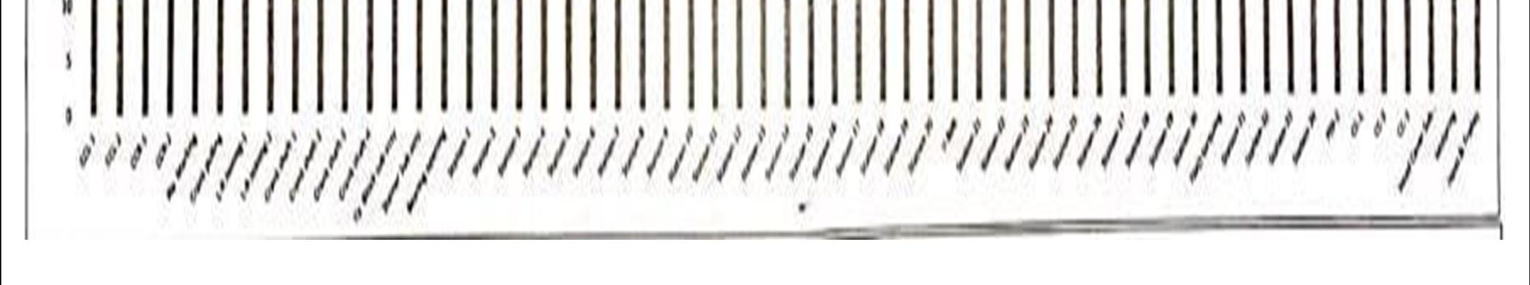
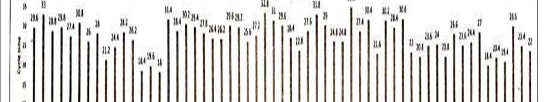
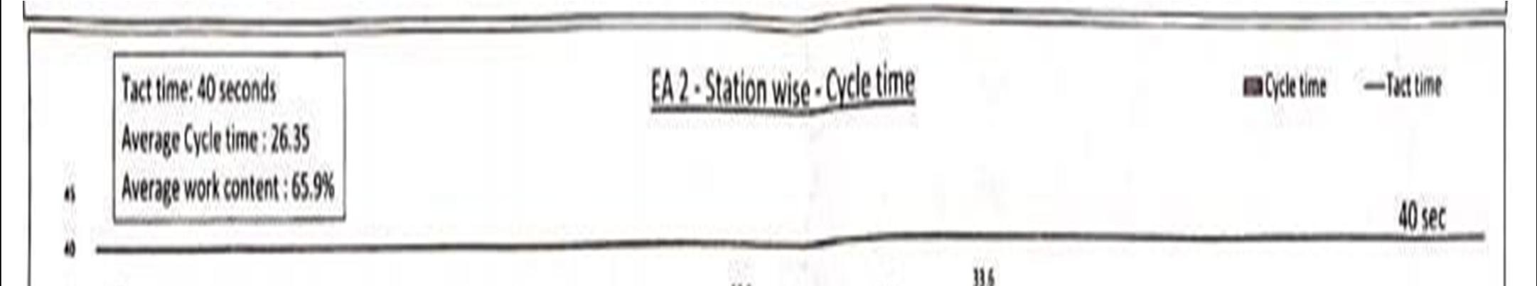
1) Station wise cycle Time Chart: Each engine assembly is processed at a station for a certain amount of time known as the "Station Cycle Time." Compared to automated stations, manual stations have somewhat longer cycle times and more fluctuating cycle times. A station's cycle time is determined using a variety of factors as shown in Figure 5. The cycle time would be longer the more complicated and numerous the activities that needed to be completed at a station. The "Line Rate," or the number of engines to be produced per unit of time, is a crucial factor in deciding which assembly activities should be delegated to which stations. The target yearly vehicle assembly volumes are often used to establish this value. Based on production volume and shift patterns used in the plant, the line rate is also represented in terms of seconds per engine.

Figure 5 Station wise Cycle time chart [23]

ISSN: 2321 9653; IC Value: 45.98; SJ Impact Factor: 7.538 Volume 10 Issue XI Nov 2022 Available at www.ijraset.com

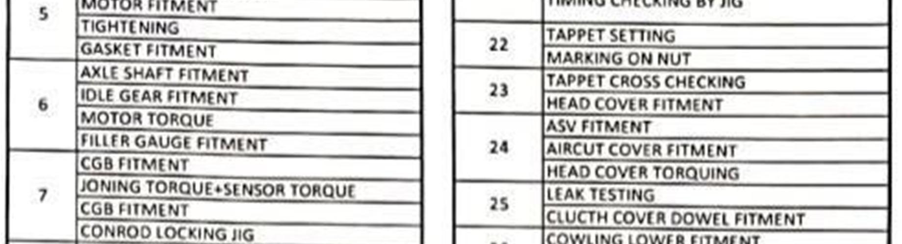
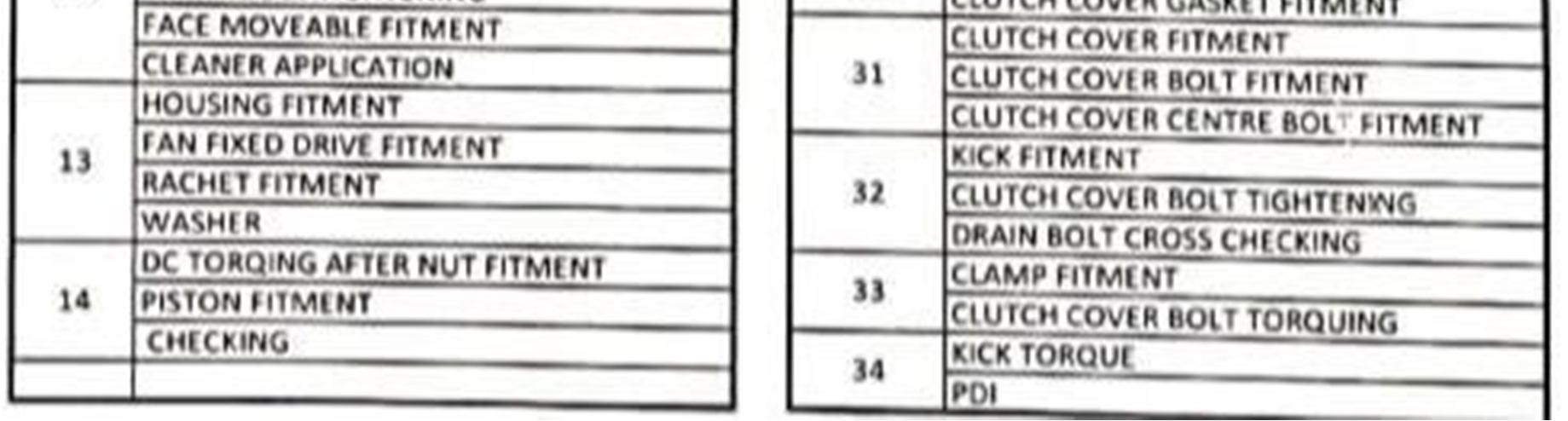
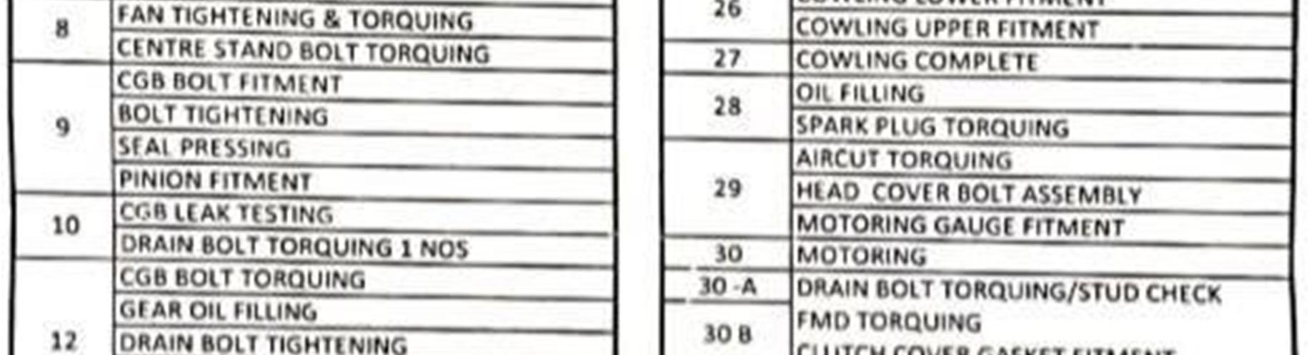
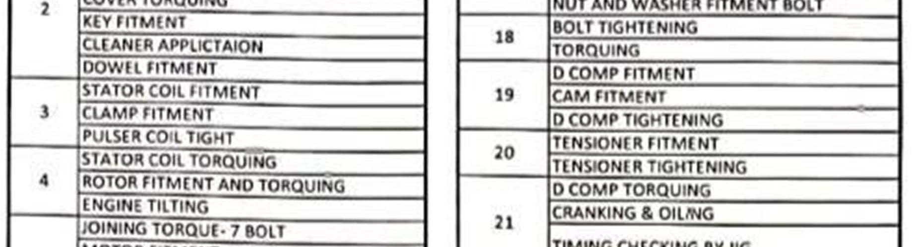
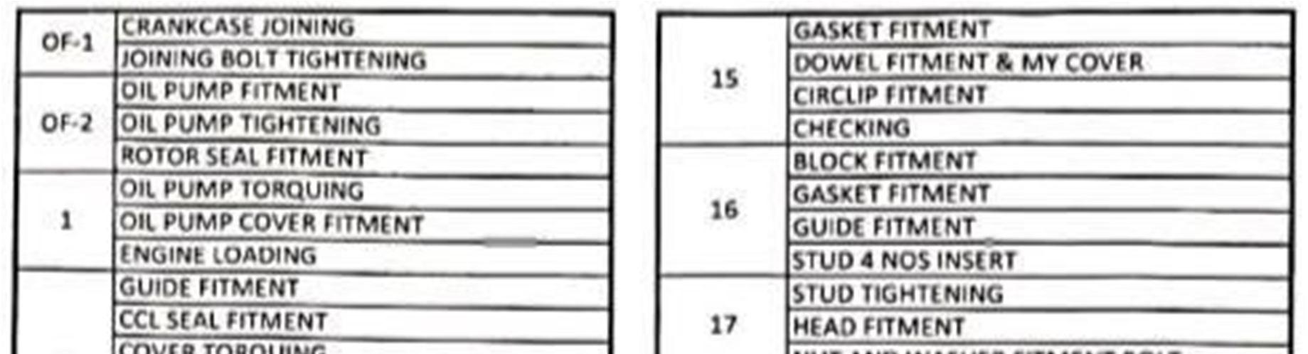
2) Station Wise Cycle Datasheet: Each station has a specific task as shown in Figure 6. Most of these tasks are arranged in order to ease reachability to several major components and in a proper sequence (i.e., dashboard before sheet).

Figure 6 Station Wise Cycle Datasheet [23]

International Journal for Research in Applied Science & Engineering Technology (IJRASET)

ISSN: 2321 9653; IC Value: 45.98; SJ Impact Factor: 7.538 Volume 10 Issue XI Nov 2022 Available at www.ijraset.com

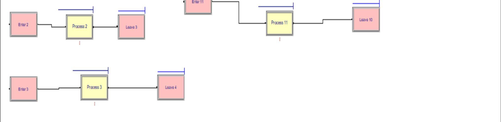
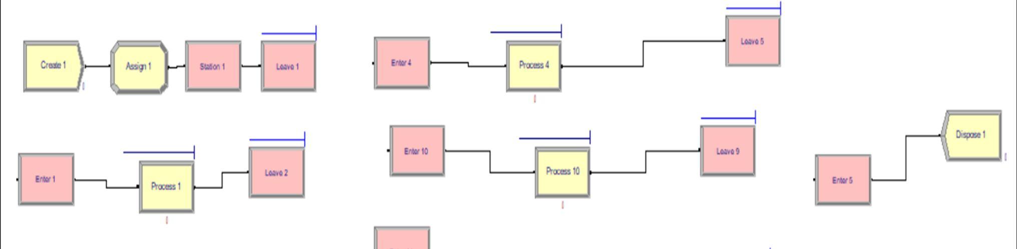
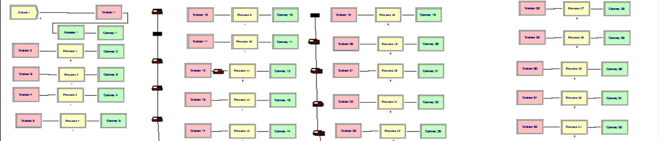
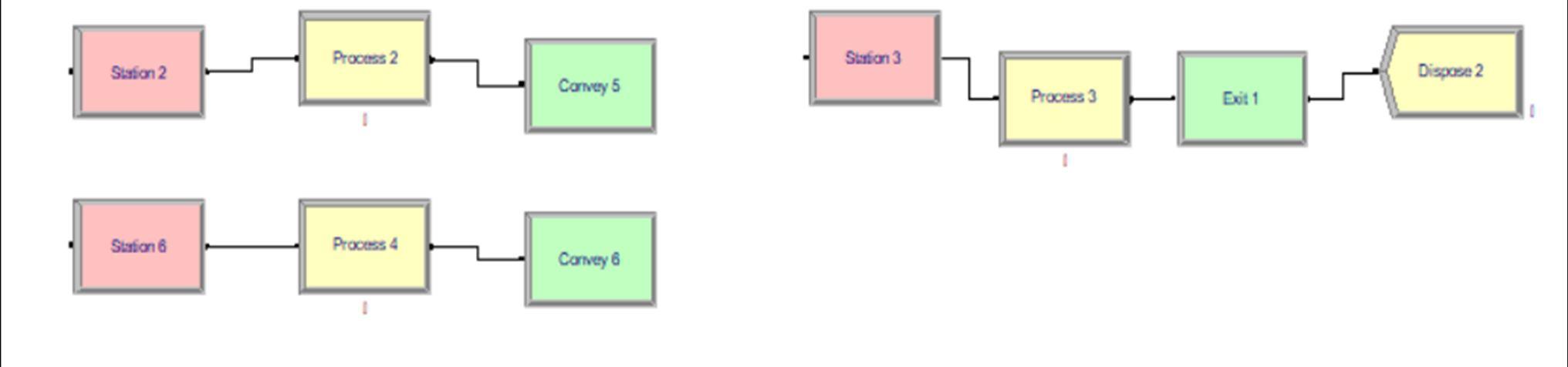
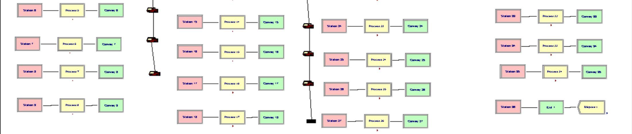
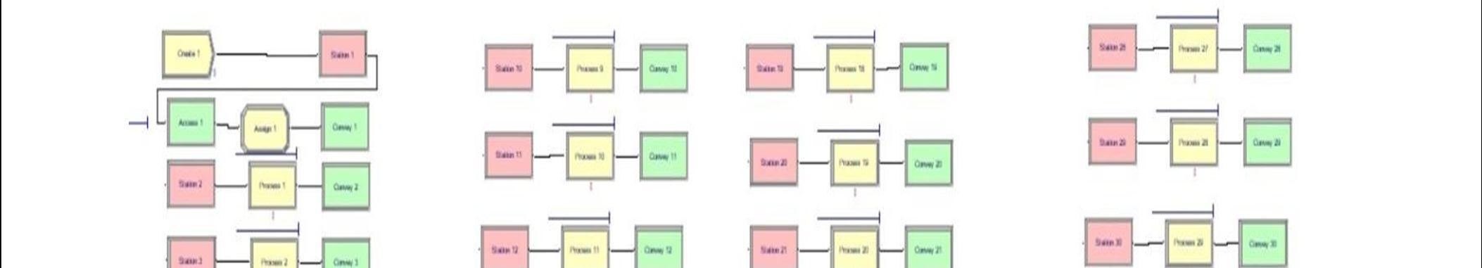
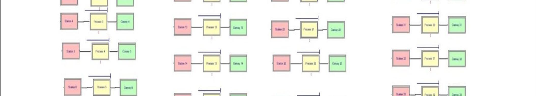
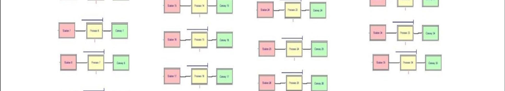
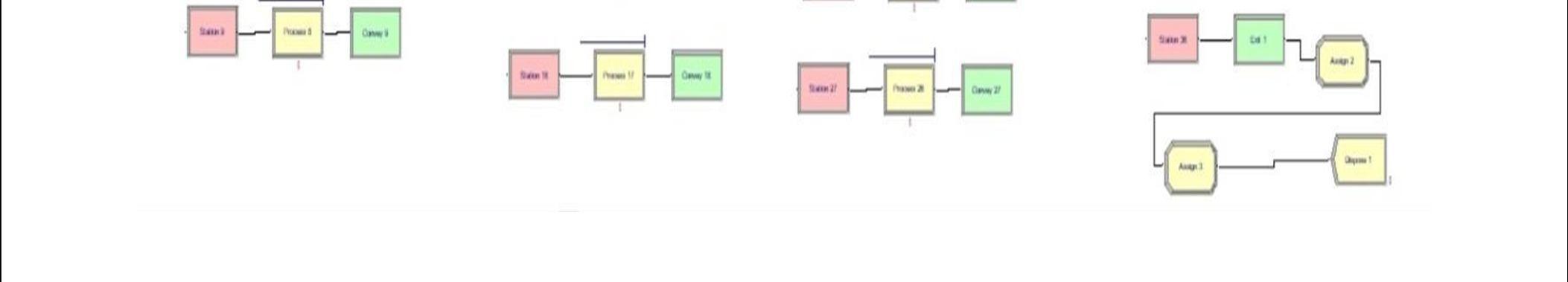
F. Model for 34 station Assembly System of the single cylinder S.I. Engine

Figure 7 Assembly line model

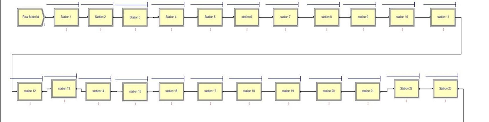
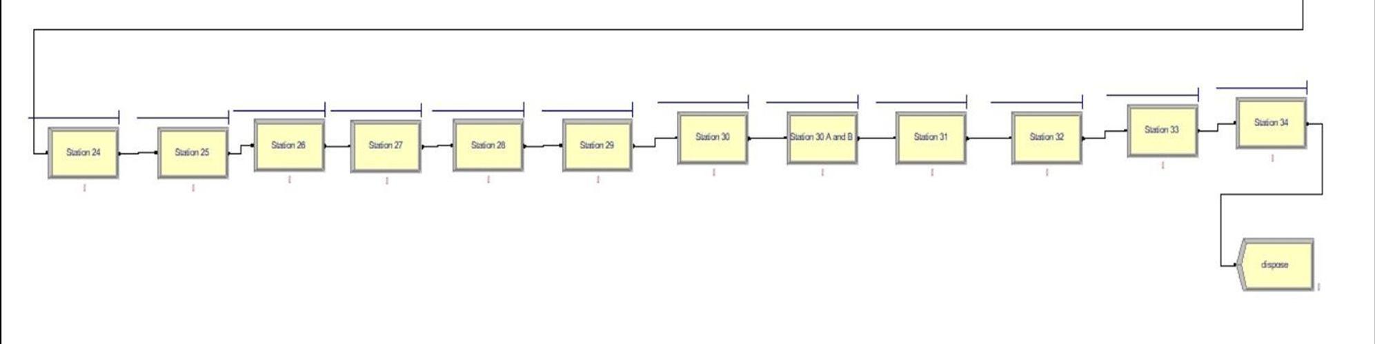
The sequence of the Production line for Single cylinder S.I Engine is shown in Figure 7 and contains 34 stations

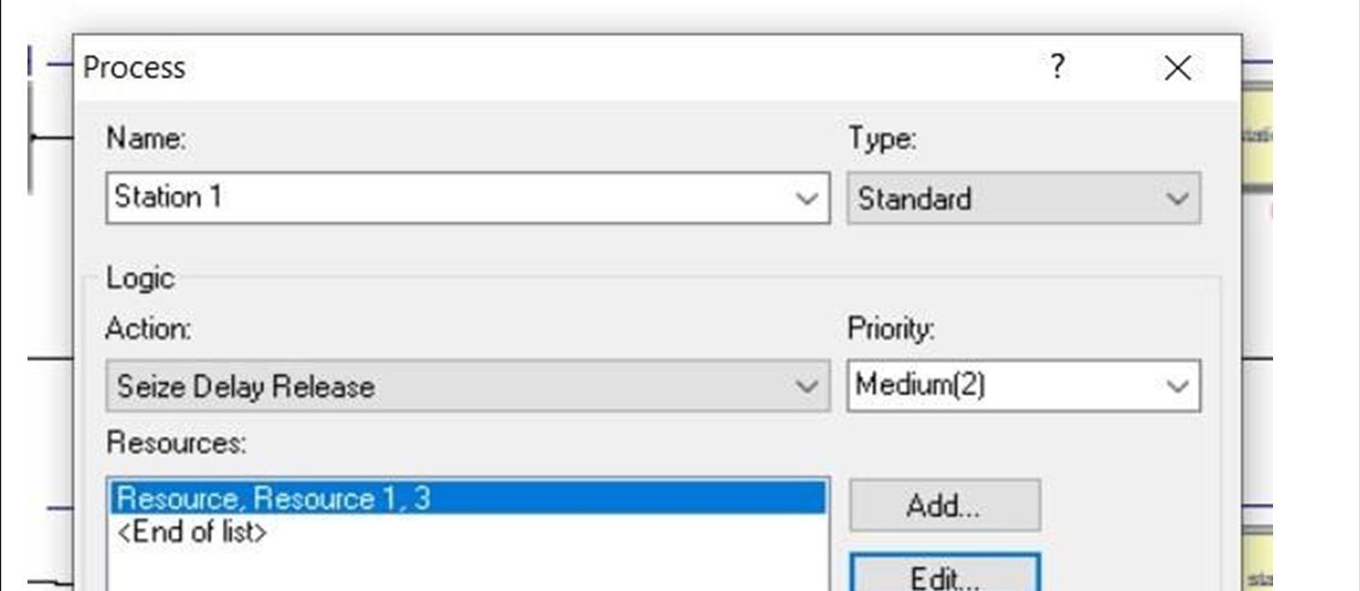
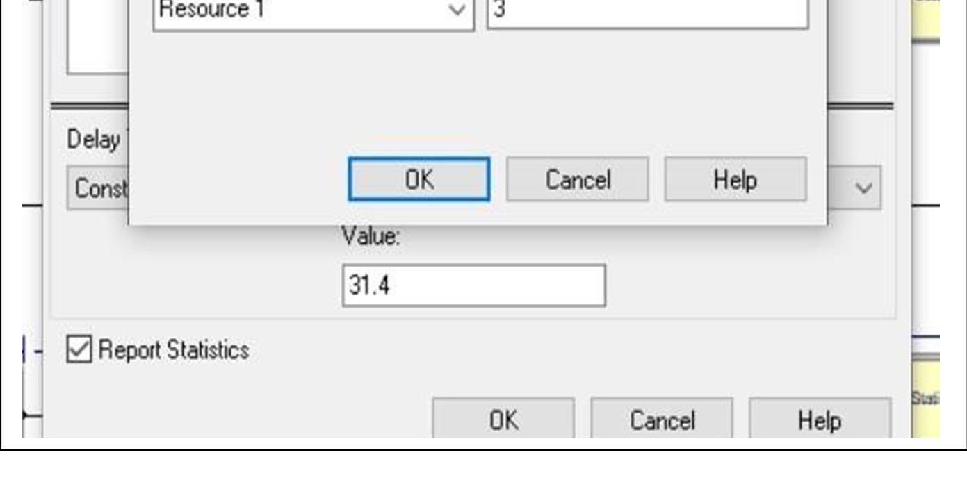
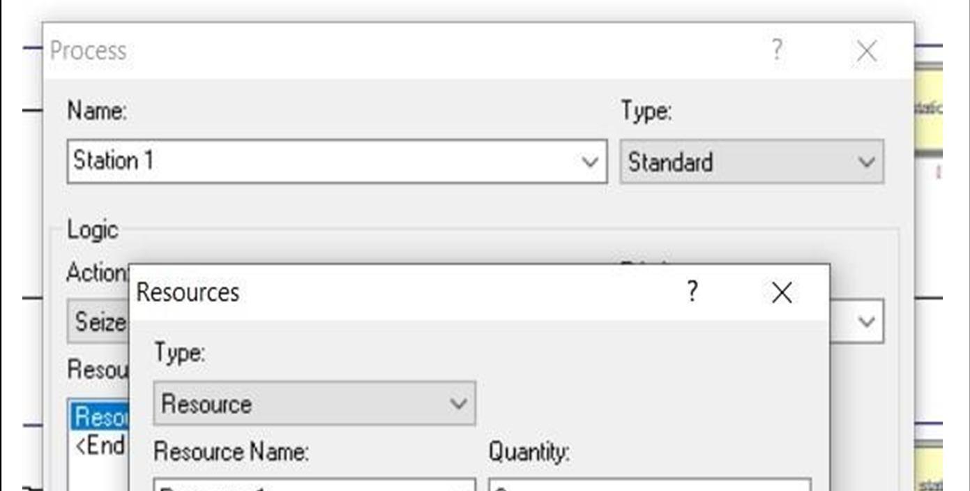
The setting parameters are Seize Delay Release with Medium Priority as shown in Figure 8.

ISSN: 2321 9653; IC Value: 45.98; SJ Impact Factor: 7.538

Volume 10 Issue XI Nov 2022 Available at www.ijraset.com

Figure 9 Resource Parameters

Details about the model

1) Each station is assigned a unique station number.

2) The "seize delay release" type of logic action has been selected for each station.

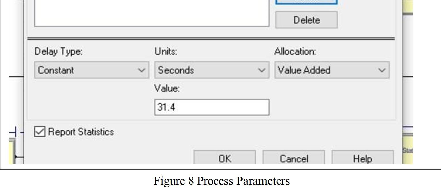
3) For each station, the kind of delay remains consistent.

4) The delay time is measured in seconds, and each station is assigned a value based on information provided by the firm as shown in Figure 5

5) Value added allocation is the selection.

6) Each station is given a specific resource name.

7) As specified in the particular datasheet as shown in Figure 6, the amount or number of operations is fixed.

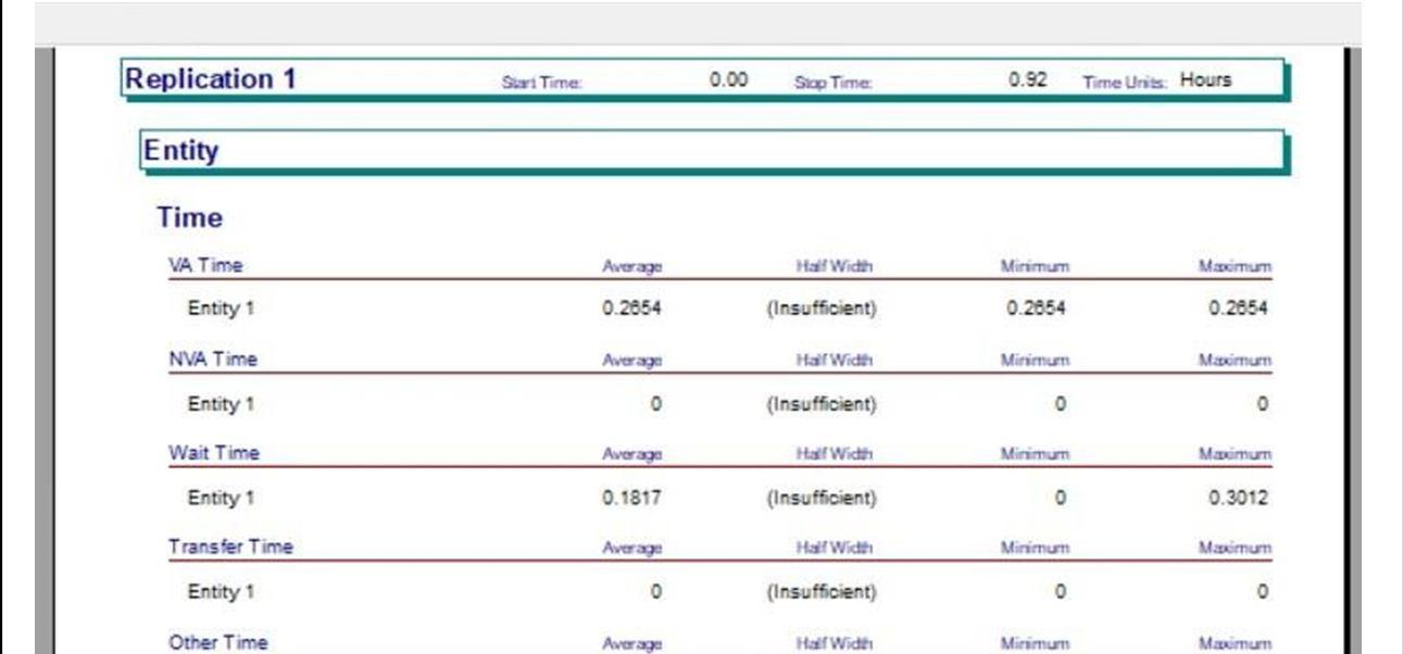
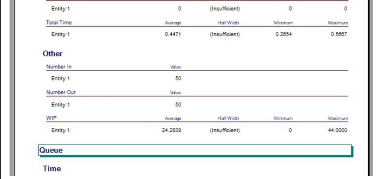
8) Information regarding the number of units, raw material build up, and disposal time is also supplied with reference to the firm information.

G. Model Analysis of Assembly System of Single cylinder S.I. Engine

The cycle times of a significant number of stations deviate greatly from the average cycle time. For the bearing opening operation prior to Station 1, the cycle time value with the lowest value is 18 seconds. The Station 21's maximum cycle time is 33.6 seconds. The median cycle time is 26.35 seconds, which is much longer than either the minimum or maximum cycle duration. The average work content is quite low at 65.9 percent.

International Journal for Research in Applied Science & Engineering Technology (IJRASET

ISSN: 2321 9653; IC Value: 45.98; SJ Impact Factor: 7.538 Volume 10 Issue XI Nov 2022 Available at www.ijraset.com

1) Statistical Analysis

Figure 10 Model Report in Arena Software

Figure 11 Model Report in Arena Software

Relation of Resources or Station with Total number Seized, Scheduled Utilization, Number Busy, Instantaneous Utilization, and Number Waiting show a similar trend of value over each resource as shown in Table 1.

ISSN: 2321 9653; IC Value: 45.98; SJ Impact Factor: 7.538

Volume 10 Issue XI Nov 2022 Available at www.ijraset.com

Table 1 Model report in Arena Software

Usage Total number Seized Scheduled Utilization Number Busy Instantaneous Utilization Number Waiting

Resources 1 50 0.4737 0.4737 0.4737 0.4737

Resources 2 50 0.4285 0.4285 0.4285 0.4285

Resources 3 50 0.4556 0.4556 0.4556 0.4556

Resources 4 50 0.4436 0.4436 0.4436 0.4436

Resources 5 50 0.4194 0.4194 0.4194 0.4194

Resources 6 50 0.3983 0.3983 0.3983 0.3983

Resources 7 50 0.3953 0.3953 0.3953 0.3953

Resources 8 50 0.4466 0.4466 0.4466 0.4466

Resources 9 50 0.4406 0.4406 0.4406 0.4406

Resources 10 50 0.3862 0.3862 0.3862 0.3862

Resources 11 50 0.4104 0.4104 0.4104 0.4104

Resources 12 50 0.4949 0.4949 0.4949 0.4949

Resources 13 50 0.4677 0.4677 0.4677 0.4677

Resources 14 50 0.4466 0.4466 0.4466 0.4466

Resources 15 50 0.3983 0.3983 0.3983 0.3983

Resources 16 50 0.344 0.344 0.344 0.344

Resources 17 50 0.4164 0.4164 0.4164 0.4164

Resources 18 50 0.4798 0.4798 0.4798 0.4798

Resources 19 50 0.4375 0.4375 0.4375 0.4375

Resources 20 50 0.3742 0.3742 0.3742 0.3742

Resources 21 50 0.5069 0.5069 0.5069 0.5069

Resources 22 50 0.4131 0.4131 0.4131 0.4131

Resources 23 50 0.4587 0.4587 0.4587 0.4587

Resources 24 50 0.3259 0.3259 0.3259 0.3259

Resources 25 50 0.4617 0.4617 0.4617 0.4617

Resources 26 50 0.4285 0.4285 0.4285 0.4285

Resources 27 50 0.4617 0.4617 0.4617 0.4617

Resources 28 50 0.3319 0.3319 0.3319 0.3319

Resources 29 50 0.3138 0.3138 0.3138 0.3138

Resources 30 100 0.7182 0.7182 0.7182 0.7182

Resources 31 50 0.3138 0.3138 0.3138 0.3138

Resources 32 50 0.4013 0.4013 0.4013 0.4013

Resources 33 50 0.3561 0.3561 0.3561 0.3561

Resources 34 50 0.3681 0.3681 0.3681 0.3681

ISSN: 2321 9653; IC Value: 45.98; SJ Impact Factor: 7.538 Volume 10 Issue XI Nov 2022 Available at www.ijraset.com

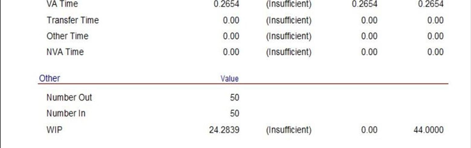
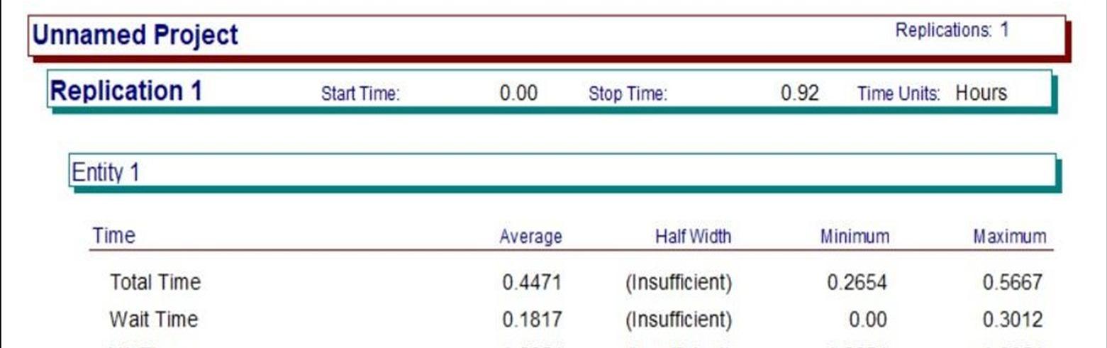
Waiting Number per Station is shown in Table 2 with the average waiting number ranging from around 0 to 3.7257. with Station 30B having a Maximum value of 11.

Table 2 Other model report in Arena Software

Number Waiting Average Half Width Minimum Maximum

Station 1 1.9961 (Insufficient) 0 9 Station 2 0 (Insufficient) 0 0 Station 3 0 (Insufficient) 0 0 Station 4 0 (Insufficient) 0 0 Station 5 0 (Insufficient) 0 0 Station 6 0 (Insufficient) 0 0 Station 7 0 (Insufficient) 0 0 Station 8 0 (Insufficient) 0 0 Station 9 0 (Insufficient) 0 0 Station 10 0 (Insufficient) 0 0 Station 11 0 (Insufficient) 0 0 Station 12 0.5175 (Insufficient) 0 3 Station 13 0 (Insufficient) 0 0 Station 14 0 (Insufficient) 0 0 Station 15 0 (Insufficient) 0 0 Station 16 0 (Insufficient) 0 0 Station 17 0 (Insufficient) 0 0 Station 18 0 (Insufficient) 0 0 Station 19 0 (Insufficient) 0 0 Station 20 0 (Insufficient) 0 0 Station 21 0.2957 (Insufficient) 0 2 Station 22 0 (Insufficient) 0 0 Station 23 0 (Insufficient) 0 0 Station 24 0 (Insufficient) 0 0 Station 25 0 (Insufficient) 0 0 Station 26 0 (Insufficient) 0 0 Station 27 0 (Insufficient) 0 0 Station 28 0 (Insufficient) 0 0 Station 29 0 (Insufficient) 0 0

Station 30 A 3.7257 (Insufficient) 0 10 Station 30 B 3.3066 (Insufficient) 0 11 Station 31 0 (Insufficient) 0 0 Station 32 0.04471 (Insufficient) 0 1 Station 33 0 (Insufficient) 0 0 Station 34 0 (Insufficient) 0 0

ISSN: 2321 9653; IC Value: 45.98; SJ Impact Factor: 7.538 Volume 10 Issue XI Nov 2022 Available at www.ijraset.com

2) Analysis of Operations and Process: It demonstrates that certain stations have congestion and some stations have relatively short cycle times. It also illustrates the necessity for line balancing research to cut the tact time from 40 seconds to something more in line with the typical cycle duration. It makes a comment on balancing work at a crucial point. It emphasizes the need of allocating adequate manpower to achieve the desired output rate in the shortest possible period, ideally zero. The investigation placed a strong emphasis on the growth of typical work content. Several of the crucial procedures include

a) Rotor nut tightening at Station no. 4

b) FMD Nut tightening at Station 30B.

c) Motoring at Station 30.

d) Engine leak testing at Station 25.

H. Effect of Addition Conveyer in Assembly Line

Types of Conveyors:

1) Non accumulating

a) Belt, bucket line, and escalators are examples of non accumulating conveyors. When the lead entity stops moving, the conveyor and all other entities also come to a halt.

b) The distances between the objects on it remain constant.

c) The whole conveyor stops for entity access/exit if the load/unload time exceeds 0.

2) Accumulating

a) Rolling Conveyors often have rollers.

b) The conveyor never stops rolling, and if a person or object gets off to exit, others behind them become backed up and barred (entities ahead of it keep moving without any blockage)

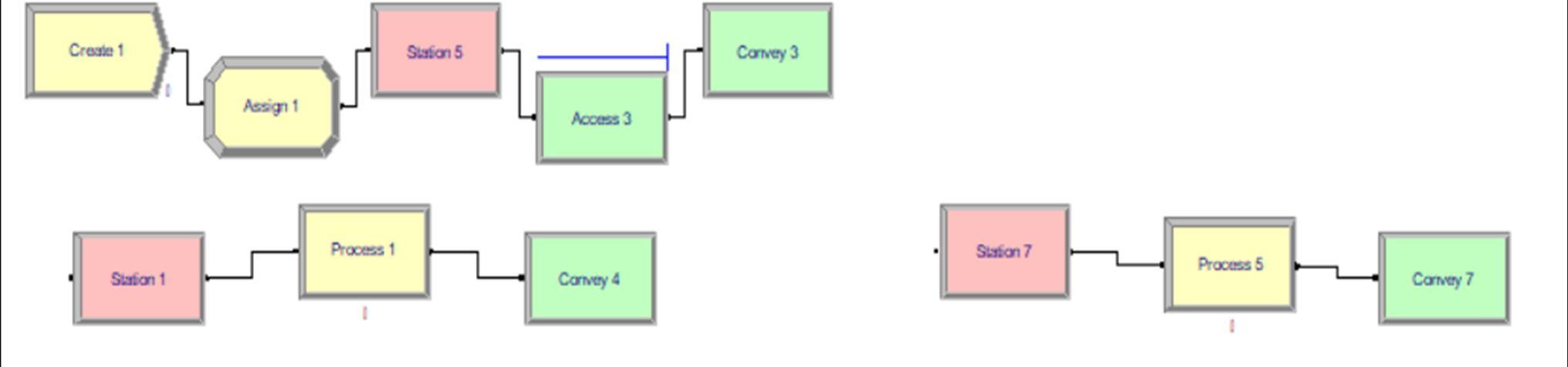
A prototype must be created before the full assembly line model can be created in order to see the results and provide a clear scenario for the subsequent steps in creating the ideal model.

 Model 1

In this concept, an accumulating conveyor is employed, but the loading and unloading of the entity are handled by an entrance and exit module to provide processing precedence at all stations as shown in Figure 12. The attribute of the sequence is provided by the assigned module, and as a result, the sequence is specified in the sequence module before transfer. Since the conveyor starts at this same process station, there is a significant seize delay and release delay at the initial process.

Figure 12 Example Model 1 in Arena Software

ISSN: 2321 9653; IC Value: 45.98; SJ Impact Factor: 7.538 Volume 10 Issue XI Nov 2022 Available at www.ijraset.com

 Model 2

In this concept, an accumulating conveyor is employed, but the loading and unloading of the entity are handled by an entrance and exit module to provide processing precedence at all stations as shown in Figure 13. The attribute of the sequence is provided by the assigned module, and as a result, the sequence is specified in the sequence module before transfer. Since the conveyor starts at this same process station, there is a significant seize delay and release delay at the initial process.

Figure 13 Example Model 2 in Arena Software

 Model 3

The conveyor in this type is non Accumulating, and the modules are Access and Convey as Shown in Figure 14. By doing this, the conveyor may travel synchronously and the Work in Process Inventory is decreased to zero. Entities create a line solely at the conveyor entry, which may be readily controlled to reach optimal manufacturing output, drastically cutting down on waiting times. The job is done directly on the conveyor, therefore there is no loading or unloading time in the model. When compared to alternative models, this results in a lower number for WIP and a lower overall average cycle time.

Figure 14 Example Model 3 in Arena Software

ISSN: 2321 9653; IC Value: 45.98; SJ Impact Factor: 7.538

Volume 10 Issue XI Nov 2022 Available at www.ijraset.com

I. Synchronous Movement of Conveyor:

When the conveyor moves synchronously, all of the objects move along it at the same time. The conveyor won't move until all of the entities have been processed at all of the stations if one entity is being processed at one station before all of the others.

1) The entities go together to the next station.

2) The things only travel along the conveyor when all of the stations' tasks have been finished.

3) The conveyor's movement is based on which Station requires the longest processing time.

4) To do this, all entities are put on a conveyor that doesn't accumulate and processed there.

5) Because the job is done on the conveyor itself, there is no loading or unloading time.

6) Significantly less time is spent waiting for the items in the queue.

7) The entities' WIP Inventory is zero now.

J. Final Arena Model Animation

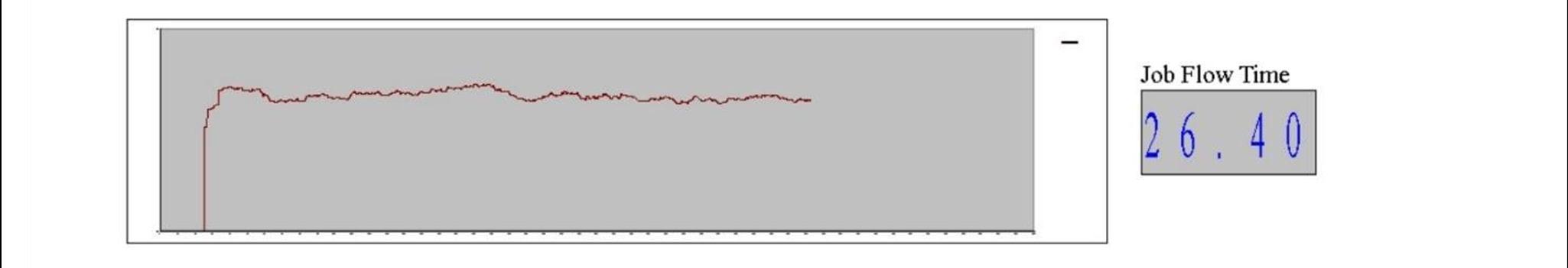
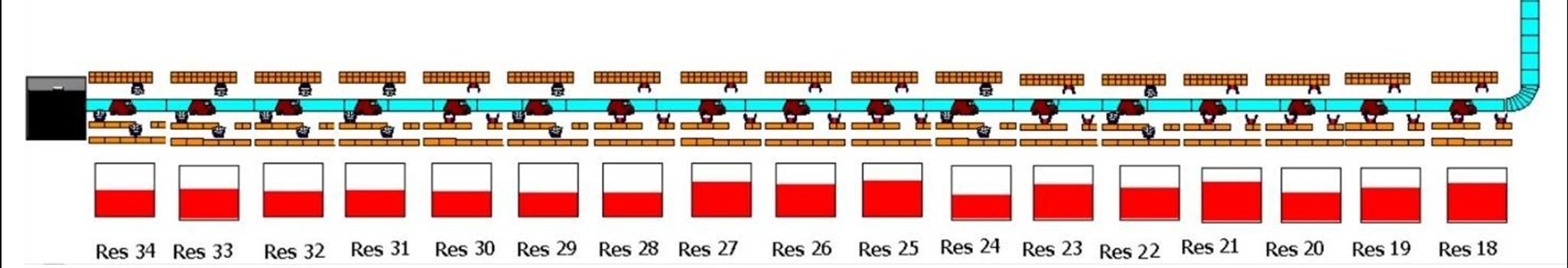
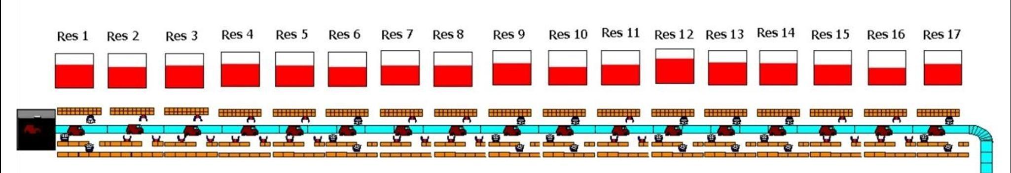
The final model's animation displays several assembly line performance metrics that enable us to assess the efficiency of the line as shown in Figure 15. The following traits may be noticed in the animation:

Job Flow Time: This is the amount of time it takes an entity to complete all of its tasks. It is equal to how long it takes to make one automobile from start to finish.

Resource utilization measures how much of the time a resource is used. It is comparable to how many people are working at a certain station as shown in Figure 16

Figure 15 Final Model in Arena Software

ISSN: 2321 9653; IC Value: 45.98; SJ Impact Factor: 7.538

Volume 10 Issue XI Nov 2022 Available at www.ijraset.com

Figure 16 Final Model Animation in Arena Software

The following benefits are provided by including the Conveyor in the model:

1) Provides synchronized entity movement, which shortens the duration of the entire operation and improves working effectiveness.

2) Conveyors are used to decrease the amount of work in progress inventory and boost output.

3) Scheduling the use of the resources.

4) It aids in lowering the chance of harm, hence ensuring a secure working environment for the employees.

5) By effectively using the working area, it creates extra room for work.

IV. RESULT AND DISCUSSION

1) Line balancing research is necessary to cut the tact time from 40 seconds to something more in line with industry standards.

2) Balance of work is necessary for key stations.

3) By balancing processes, you may directly save on labor

4) Defect management reduces the need for repair personnel.

5) Reduce the station process time's deviation from the average cycle time as much as possible.

6) The content of work overall has improved.

The different improvements indicated are highlighted by the simulation model and research analysis in order to boost throughput and production rate. A regular schedule must be followed for maintenance and effective manpower use. The project's goal is to avoid bottlenecks and hunger so that the single cylinder S.I. engine assembly line system will operate effectively. Additional research has to be done:

a) Variability in process duration and its impact on the product.

b) Redesigning aspects of the job and its impact on output.

c) Investigate whether deploying resources at the assembly station enhances system performance.

A.

Variability in process times

Utilizing a triangle or expression type delay will allow for process time diversity. And in doing so, it is ensured that the variability percentage at each of the 34 sites is the same. In order to determine the general criteria for the variation in resource utilization and other characteristics according to variation in process time, we will examine the 4 scenarios as shown in Figure 17.

ISSN: 2321 9653; IC Value: 45.98; SJ Impact Factor: 7.538 Volume 10 Issue XI Nov 2022 Available at www.ijraset.com

Process time variability enables:

1) To account for supply and demand in different market situations when calculating the average cycle time. 2) To get a sense of how resources are used under various circumstances. 3) To increase the system's adaptability.

4) Establishing a connection between the variability percentage, the overall average cycle time, and the WIP.

Variation of Job flow time with % Variability:

25.4241 30.8632 36.7073 42.9678

Job Flow Time % Variability

Figure 17 Job Flow Time vs percent Variability

Variations among the different percent of Variability with respect to Job Flow time Show max time at 20 percent variability with a value of 42.9678 and the Lowest time taken was at 5 percent variability with a value being 25.4241 as shown in Figure 17

B. Resource Utilization:

1) Variability 5%

The relation of Utilization and Resources at 5 percent variability is shown in Figure 18, which shows the lowest value of 0.4499 and the highest value of 0.7348.

Resource

ISSN: 2321 9653; IC Value: 45.98; SJ Impact Factor: 7.538 Volume 10 Issue XI Nov 2022 Available at www.ijraset.com

2) Variability 10%

The relation of Utilization and Resources at 10 percent variability is shown in Figure 19, which shows the lowest value of 0.3678 and the highest value of 0.6080.

Utilization

Utilization

Figure 19 Resource vs 10 percent Variability

3) Variability

15%

The relation of Utilization and Resources at 10 percent variability is shown in Figure 20, which shows the lowest value of 0.3254 and the highest value of 0.5129.

Utilization

Utilization

Figure 20 Resource vs 15 percent Variability

ISSN: 2321 9653; IC Value: 45.98; SJ Impact Factor: 7.538

Volume 10 Issue XI Nov 2022 Available at www.ijraset.com

4) Resource Utilization Data

The relation of different percent of Variabilityis shown in Table 4 with an average being 0.5936 at 5 percent variability,0.4938 at 10 percent variability, and 0.4204 at 15 percent variability. Resource utilization value reduces as variability percent increases.

Table 3 Resource Utilization Data 5 % 10 % 15 %

Resource 1 0.6820 0.5687 0.4857

Resource 2 0.6174 0.5108 0.4367

Resource 3 0.6592 0.5405 0.4602

Resource 4 0.6397 0.5305 0.4457

Resource 5 0.6058 0.4999 0.4349

Resource 6 0.5721 0.4828 0.4142

Resource 7 0.5714 0.4770 0.4046

Resource 8 0.6426 0.5409 0.4488

Resource 9 0.6384 0.5247 0.4543

Resource 10 0.5567 0.4554 0.4001

Resource 11 0.5874 0.4855 0.4132

Resource 12 0.7108 0.5938 0.4982

Resource 13 0.6781 0.5605 0.4681

Resource 14 0.6460 0.5379 0.4502

Resource 15 0.5726 0.4783 0.4013

Resource 16 0.4967 0.4069 0.3519

Resource 17 0.5971 0.4978 0.4229

Resource 18 0.6944 0.5775 0.4823

Resource 19 0.6325 0.5197 0.4482

Resource 20 0.5376 0.4441 0.3943

Resource 21 0.7348 0.6080 0.5129

Resource 22 0.5973 0.4870 0.4142

Resource 23 0.6616 0.5569 0.4700

Resource 24 0.4692 0.3964 0.3355

Resource 25 0.6640 0.5489 0.4690

Resource 26 0.6157 0.5131 0.4308

Resource 27 0.6669 0.5466 0.4585

Resource 28 0.4795 0.4042 0.3286

Resource 29 0.4499 0.3678 0.3254

Resource 30 0.5129 0.4298 0.3656

Resource 31 0.5257 0.4248 0.3721

Resource 32 0.4549 0.3765 0.3268

Resource 33 0.5825 0.4734 0.4032

Resource 34 0.5196 0.4236 0.3660

ISSN: 2321 9653; IC Value: 45.98; SJ Impact Factor: 7.538 Volume 10 Issue XI Nov 2022 Available at www.ijraset.com

V. CONCLUSION

The study's objective was to show how simulation can assess various scenarios and gauge a car assembly line's performance. This study also demonstrates how to create a model of a complex assembly line and its feeder stations utilizing the basic data modules in simulation software like ARENA. Additionally, ARENA's animation and debug features may be used to verify the model's accuracy and usefulness. A quadratic model for line production dependent on operator fatigue, conveyor speed, and incoming material quality was proposed using data analysis. The analysis identifies the system's numerous bottlenecks and also makes note of the areas that need more thought. The analyst can use this model to forecast how changes to the system will affect the system. This simulation model, which represents how an assembly method currently in use for single cylinder S.I. engines operates in terms of time, aids in performance analysis.

The third model, which substitutes convey for entrance and exit, offers us a clear concept of the model to be constructed. Due to the model's simplicity and similar resemblance to the one utilized by the corporation. The advantage of using a conveyor is that it eliminates the extra time that was required for product entrance and exit at Model 1, which allows us to reduce the time that the job is in process. When compared to a model that used convey instead of entrance and leave, the model using entry and leave had a greater average cycle duration and less work in progress. This is mostly caused by the product being continuously loaded and unloaded at each station. The time spent in line is also significantly decreased. This is due to the model's conversion to an accumulating type. When comparing the two, the one with the conveyor has a significantly lower amount of work in progress than the one without.

This is due to effective resource usage and the fact that the product doesn't get taken off the conveyor at each station but rather stays in line. Understanding how to do away with the non value added time of loading and unloading the product from the line is also helpful. The job flow time grows along with the variance in process time. Resource Utilization reduces as variety increases. This demonstrates how the outcomes deviate from an ideal model as we approach reality. By adopting synchronized conveyor movement, certain stations' resource use is higher than average while other stations' resource utilization is lower than normal. To lessen the workload on employees at stations with high use, this necessitates workforce balance at the stations.

REFERENCES

[1] Benedettini O, Tjahjono B (2009) Towards an improved tool to facilitate simulation modelling of complex manufacturing systems. Int J Adv Manuf Technol 43:191 199, Springer

[2] Villa A, Ares Gómez JE (1987) A methodology to analyze workshop lines by discrete event dynamic models. In: Mital A (ed) 9th International Conference on Production Research, vol I. ICPR, Cincinnati, pp 2072 2078.

[3] Shannon RE (1998) Introduction to the Art and Science of Simulation. In: Medeiros DJ, Watson EF, Carson JS, Manivannan MS (eds) Proceedings of 1998 Winter Simulation Conference. IEEE, Baltimore

[4] Ingalls RG (2001) Introduction to Simulation. In: Peters BA, Smith JS, Medeiros DJ, Rohrer MW (eds) Proceedings of the 2001 Winter Simulation Conference. IEEE, Baltimore

[5] Andersson M, Olsson G (1998) A Simulation based decision support approach for operational capacity planning in a customer order driven assembly line. In: Medeiros DJ, Watson EF, Carson JS, Manivannan MS (eds) Proceedings of the 1998 Winter Simulation Conference. IEEE, Baltimore

[6] Ladbrook J, Tjahjono B, Oakes E, de Sanabria Sales RR, Garcia de Rueda A, Lizarazu U, and Temple C (2011) Simulation Study for Investment Decision of the EcoBoost Camshaft Machining Line. J Eng Manuf, in press.

[7] P. Faget, U. Eriksson and F. Herrmann, "Applying discrete event simulation and an automated bottleneck analysis as an aid to detect running production constraints," Proceedings of the Winter Simulation Conference, 2005., 2005, pp. 7 pp. , doi: 10.1109/WSC.2005.1574404.

[8] Roser, C., Nakano, M. and Tanaka, M. 2001. A practical bottleneck detection method. In Proceedings of the 2001 Winter Simulation Conference, ed. B. A. Peters, J. S. Smith, D. J. Medeiros, and M. W. Rohrer, 949 953. Piscataway, New Jersey: Institute of Electrical and Electronics Engineers. Available via [accessed April 10, 2005]

[9] Jayaraman, A. and Agarwal, A. (1996) ‘Simulating an engine plant’, Manufacturing Engineering, Vol. 117, No. 5, p.60

[10] Darayi, M., Eskandari, H. and Geiger, C.D. (2013) ‘Using simulation based optimization to improve performance at a tire manufacturing company’, QScience Connect (a Qatar foundation academic journal), pp.1 12.

[11] Sarda, Akshay & Digalwar, Abhijeet. (2018). Performance analysis of vehicle assembly line using discrete event simulation modelling. International Journal of Business Excellence. 14. 240. 10.1504/IJBEX.2018.10009766.

[12] Jayaraman, A. and Gunal, A.K. (1997) ‘Applications of simulation in the design of automotive manufacturing systems’, Proceedings of the 1997 Winter Simulation Conference, pp.758 764.

[13] Shrouf, F., Ordieres, J., & Miragliotta, G. (2014). Smart factories in Industry 4.0: A review of the concept and of energy management approached in production based on the Internet of Things paradigm. Paper presented at: Industrial Engineering and Engineering Management (IEEM), 2014 IEEE International Conference on (IEEE), Bandar Sunway, Malaysia

[14] Rüßmann, M., Lorenz, M., Gerbert, P., Waldner, M., Justus, J., Engel, P., & Harnisch, M. (2015). Industry 4.0: The future of productivity and growth in manufacturing industries. Boston Consulting Group, 9, 1 16.

[15] Tortorella, M. (2005). Service reliability theory and engineering, II: Models and examples. Quality Technology & Quantitative Management, 2, 17 37.

Technology (IJRASET)

ISSN: 2321 9653; IC Value: 45.98; SJ Impact Factor: 7.538 Volume 10 Issue XI Nov 2022 Available at www.ijraset.com

[16] Cui, L., Chen, Z., & Gao, H. (2018). Reliability for systems with self healing effect under shock models. Quality Technology & Quantitative Management, 15, 551 567

[17] Ingalls RG (2001) Introduction to Simulation. In: Peters BA, Smith JS, Medeiros DJ, Rohrer MW (eds) Proceedings of the 2001 Winter Simulation Conference. IEEE, Baltimore

[18] Becker, J. M. J., Borst, J., & van der Veen, A. (2015). Improving the overall equipment effectiveness in high mixlow volume manufacturing environments. CIRP Annals Manufacturing Technology, 64, 419 422.

[19] Douard D, Baynat B (2002) Improving Efficiency of Decomposition Methods for Closed Loop Continuous Flow Production Models. ACS’02 SCM Conference, Poland, October 23 25

[20] Xu, K., Xie, M., Tang, L. C., & Ho, S. (2003). Application of neural networks in forecasting engine systems reliability. Applied Soft Computing, 2, 255 268.

[21] https://www.tutorialspoint.com/modelling_and_simulation/modelling_and_simulation_verification_validatio n.htm

[22] IEEE https://ieeexplore.ieee.org/document/1371297

[23] Maruti Suzuki EA 2 Chart