The Effect of Government Regulations on Overall Economic Well Being in India (1995-2020)

10 VII July 2022 https://doi.org/10.22214/ijraset.2022.45592

1) Rajan Sudesh Ratna and Martina Francesca Ferracane: According to them there is existingliterature on the contribution of trade facilitation to the enhancement of trade as well as to the promotion of GDP growth, welfare improvements and government revenue, all of which go a long way towards poverty reduction. However, the government role is found to be crucial in ensuring that the poor fullybenefit from the increased trade opportunities.

International Journal for Research in Applied Science & Engineering Technology (IJRASET) ISSN: 2321 9653; IC Value: 45.98; SJ Impact Factor: 7.538 Volume 10 Issue VII July 2022 Available at www.ijraset.com 5023©IJRASET: All Rights are Reserved | SJ Impact Factor 7.538 | ISRA Journal Impact Factor 7.894 | The Effect of Government Regulations on Overall EconomicWell Being in India(1995-2020)

I. INTRODUCTION Trade can act as a powerful engine for economic growth and development. Developing countrieslike India have long strived for a development strategy that will sustain high economic growth, create employment opportunities and eliminate poverty. Trade policy is being used by the developing countries as a tool for attaining their development objectives, which aim to combine higher economic growth with employment generation in order to alleviate poverty. Trade facilitation is also found to have positive effects on gross domestic product (GDP), economic welfare and government revenue. Free trade is widely thought to be prerequisite for sustained economic success, but many countries feel the need to promote domestic production by enforcing barriers and regulations on imported goods and regulating different aspects of the economy as a whole. The same is true of regulation in other sectors of the economy, such as the labor and business markets: lawmakers are often compelled to protect the interests of various stakeholders at the expense of economic freedom. Overall, we will look at the impact of regulations and trade barriers on GDP per capita as we analyze whether the statement that completely free trade and deregulated markets are always the most beneficial for an economyis true or if regulation in some or all sectors is of helpas well. This research is important because it gives guidance as to how much is too much and how little istoo little when it comes to regulations and barriers. It shows the overall, broad trend relating trade freedom and economic regulations and to GDP per capita for a country. Using data from The Heritage Foundation’s Index of Economic Freedom and the World Bank, we analyze this relation. Our study focuses on regulatory efficiency and market openness, and within this the variables trade freedom, monetary freedom, and investment freedom, and by extension; FDI. We hypothesize that the overall trend will show a positive relationship between economic freedom and economic well being as measured by GDP per capita. This hypothesis operates off of the free market assumption that economies do best when they are left to run themselves. Thus,allowing trade, monetary, and investment to happen freely without regulations or interruption should result in the optimal economic conditions for countries. The testinghas been done using OrdinaryLeast Squares Method under Classical LinearRegression Model.

II. LITERATURE REVIEW

Aditi Das1 , Muskan Mohan2 , Nitya Sultania3 , Ishika Yadav4 1, 2, 3, 4Lady Shri Ram College for Women, University of Delhi

Abstract: Barriers to trade and other market regulations have long been thought to inhibit the ability of aNation’s economy to grow and prosper. We test this hypothesis using a multiple regression model and data from The Heritage Foundation and World Bank related to trade freedom and general economic regulation on a country to fully discern the impact of governmental regulation on a country’s GDP per capita. We find that GDP per capita rises significantly as a India’s business freedom and trade freedom grow. This provides strong confirmation for our hypothesis that deregulated economies experience higher levels of economic prosperity as measured by GDP per capita than their regulated counterparts and indicates that a market specific look shouldbe taken to fully understand the nuances of the results of different types of economic regulation.

2) Frankel and Romer (1999): Study provides some strong evidence in favour of the relationship between trade and growth while investigating whether the correlation between openness and growth was because openness causes growth, or because countries that grow faster tend to openup at the same time. Controlling the component of the openness due to such country characteristics as population, land area, and geographic distance that cannot be influenced by economic growth, they found that an increase of one percentage point in the openness ratio increased both the level of income and subsequent growth byaround 0.5 per cent.

International Journal for Research in Applied Science & Engineering Technology (IJRASET) ISSN: 2321 9653; IC Value: 45.98; SJ Impact Factor: 7.538 Volume 10 Issue VII July 2022 Available at www.ijraset.com 5024©IJRASET: All Rights are Reserved | SJ Impact Factor 7.538 | ISRA Journal Impact Factor 7.894 |

3) Nguyen Viet Cuong: The findings show that improvement in trade facilitation is positively correlated with exports and per capita GDP, and negatively correlated with poverty and inequality. More specifically, deterioration in trade facilitation which is measured by the increase in the number of documents required and days taken for exporting and importing a good can reduce per capita GDP, albeit to a small amount. Countries requiring a larger number ofdocuments and more time for imports and exports tend to have higher levels of poverty and inequality(measured bythe Gini index) than other countries.

4) Prabir De and Ajitava Raychaudhuri: The study reveals that there are many opportunities forthe poor and microenterprises to benefit from trade facilitation measures in Mukdahan and Nakhon Phanom provinces, especially in the agricultural, services and investment sectors. Thereis growing demand in Viet Nam and China for agricultural products, especially organic rice, tapioca, rubber, sugar and fresh fruit. Farmers and agricultural employees in the two provinces can benefit more now from trade facilitation measures by harvesting and exporting such agricultural products to Viet Nam and China via the improved road infrastructure.

Small, rich countries and more developed industrial countries tend to have the highest per capitaGDP. per capita GDP shows how much economic production value can be attributed to each individual citizen. Alternatively, this translates to a measure of national wealth since GDP market value per person also readilyserves as a prosperitymeasure.

III. DEPENDENT VARIABLE GDP PER CAPITA(BILLION USD)

International trade has occurred since the earliest civilisations began trading, but in recent yearsinternational trade has become increasingly important with a larger share of GDP devoted to exports and imports. International trade between different countries is an important factor in raising living standards, providing employment and enabling consumers to enjoy a greater varietyof goods.

Free and open trade has fueled vibrant competition, innovation, and economies of scale, allowingindividuals and businesses to take advantage of lower prices and increased choice

V. INDEPENDENT VARIABLE MONETARY FREEDOMINDEX

GDP stands for "Gross Domestic Product" and represents the total monetary value of all finalgoods and services produced within a countryduring a period of time. GDP is the most commonly used measure of economic activity. GDP as an economic indicator isused worldwide to show the economic health of a country. For low income or middle income countries, high year on year GDP growth is essential to meet the growing needs of the population. Hence, the GDP growth rate of India is an essential indicator of the country’s economic development and progress. Besides measuring the health of the economy and helping the government in framing policies, the GDP growth rate numbers are also useful for investors inbetter decision making related to investments

Monetary freedom combines a measure of price stability with an assessment of price controls. Both inflation and price controls distort market activity. Price stability without microeconomicintervention is the ideal state for the free market.

As a vital component of human dignity, autonomy, and personal empowerment, economic freedom is valuable as an end itself. Just as important, however, is the fact that monetary freedom provides a proven formula for economic progress and success. Policies that allowgreater freedom in these areas measured tend to spur growth.

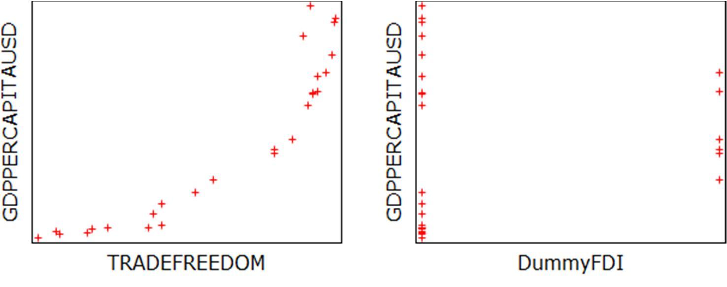
IV. INDEPENDENT VARIABLE TRADE FREEDOMINDEX

Trade freedom is a composite measure of the absence of tariff and non tariff barriers that affect imports and exports of goods and services. It measures the extent of tariff and nontariff barriers that affect imports and exports of goods and services and is calculated based on trade weighted average tariff rate and rate of non tariff barriers. An index of economic freedom measures jurisdictions against each other in terms of trade freedom, tax burden, judicial effectiveness, andso on.

A. GDP per Capita Per capita income is national income divided by population size. Per capita income is often usedto measure a sector's average income and compare the wealth of different populations. Per capitaincome is often used to measure a country's standard of living. Per capita GDP is a global measure for gauging the prosperity of nations and is used by economists, along with GDP, to analyze the prosperityof a countrybased on its economic growth.

This variable is measured on a scale from 0 100 with 100 indicating a perfectly free market and 0 indicating a completely regulated or unfree market. The score for the monetary freedom component is based on two factors: The weighted average inflation rate for the most recent threeyears and Price controls. Higher index values denote price stability without microeconomic intervention.

B. Data Source

The Indian Government’s favourable policy regime and robust business environment has ensuredthat foreign capital keeps flowing into the country. The Government has taken many initiatives in recent years such as relaxing FDI norms across sectors such as defense, PSU oil refineries, telecom, power exchanges, and stock exchanges, among others.

One Dependent And Three Explanatory VariablesMultiple Linear Regression Model  Interpretation

International Journal for Research in Applied Science & Engineering Technology (IJRASET) ISSN: 2321 9653; IC Value: 45.98; SJ Impact Factor: 7.538 Volume 10 Issue VII July 2022 Available at www.ijraset.com 5025©IJRASET: All Rights are Reserved | SJ Impact Factor 7.538 | ISRA Journal Impact Factor 7.894 |

1) The Heritage Foundation’s Index of Economic Freedom

Multiple Linear Regression, Double Log Regression, Dummy Variable and Interactive DummyVariable Regression using Ordinary Least Squares Method under the assumptions of Classical Linear Regression Model. Linear Model

Effect of India’s Trade Freedom, Monetary Freedom, and Investment Freedom on its GDP percapita (billion USD) Y: GDP per capita (billion USD)X2i :Trade Freedom (index) X3i : Monetary Freedom (index) X4i : Investment Freedom (index)

A country having freedom from restrictions on the movement and use of investment capital, regardless of activity, within and across the country's borders, & where individuals and firms would be allowed to move their resources into and out of specific activities, both internally andacross the country’s borders, without restriction. Such an ideal country would receive a score of100 on the investment freedom component of the Index of Economic Freedom.

2) The World Bank C. Methodology and Results

VII. DUMMY VARIABLE FOREIGN DIRECTINVESTMENT

Secondary data has been collected for all the variables from 1995 2020.Following are the sources of the data:

Foreign direct investment (FDI) is an investment from a party in one country into a business or corporation in another country with the intention of establishing a lasting interest. Lasting interest differentiates FDI from foreign portfolio investments, where investors passively hold securities from a foreign country. A foreign direct investment can be made by obtaining a lastinginterest or by expanding one’s business into a foreign country. Foreign direct investment offers advantages to both the investor and the foreign host country.These incentives encourage both parties to engage in and allow FDI. Foreign Direct Investment (FDI) has been a major non debt financial resource for the economicdevelopment of India. Foreign companies invest in India to take advantage of relatively lower wages, special investment privileges like tax exemptions, etc. For a country where foreign investment is being made, it also means achieving technical know how and generating employment.

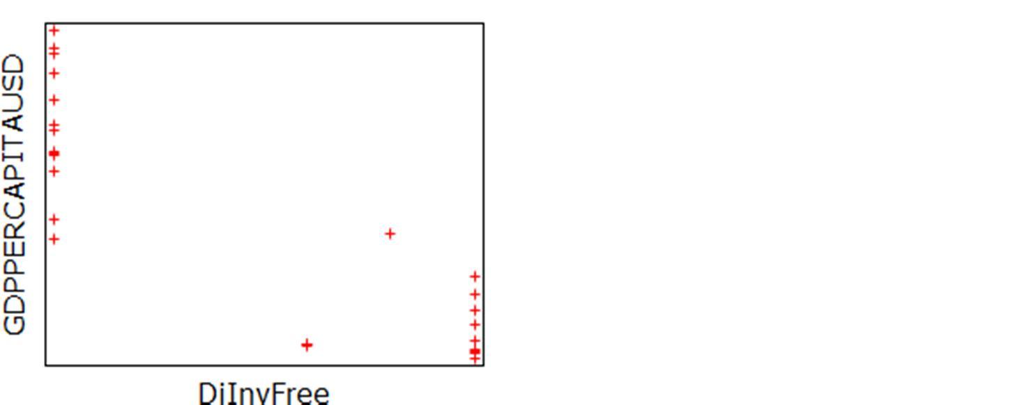
VI. INDEPENDENT VARIABLE INVESTMENT FREEDOMINDEX

A. Objective To determine the impact of India’s Trade Freedom, Monetary Freedom, InvestmentFreedom, and Foreign Direct Investment on its GDP per capita (billion USD).

In practice, most countries have a variety of restrictions on investment; restrict access to foreignexchange; impose restrictions on payments, transfers, and capital transactions.

Investment freedom refers to constraints associated with the flow of investment capital within a country. It is generated as a composite of a nation’s treatment or screening of foreign investment,foreign investment code, restrictions on land ownership, capital controls, and other factors related to investment. This variable is measured on a scale from 0 100 with 100 indicating a perfectly free market and 0 indicating a completelyregulated or unfree market.

VIII. EMPIRICAL ANALYSIS

International Journal for Research in Applied Science & Engineering Technology (IJRASET) ISSN: 2321 9653; IC Value: 45.98; SJ Impact Factor: 7.538 Volume 10 Issue VII July 2022 Available at www.ijraset.com 5026©IJRASET: All Rights are Reserved | SJ Impact Factor 7.538 | ISRA Journal Impact Factor 7.894 | Y ^ (Y Hat) = −3998.06 + 101.152X2i 29.6823X3i + 6.49479 X4i Y = β1 +β2X2i + β3X3i + β4X4i + ui , (where β2, β3, β4 are the parameters and ui is the random error term) β1 is the mean value of GDP per capita when there is no Trade, Monetary and InvestmentFreedom β2, β3, and β4 are the partial slope coefficients of mean GDP per capita w.r.t Trade, Monetary andInvestment Freedom Estimated equation Y ^ (Y Hat) = b1 + b2X2i + b3X3i + b4X4i, (where b1, b2, b3, and b4 are estimators of β1, β2 and β3, β4 respectively)  Apriori Expectations of Partial Coefficients Here, apriori expectations of β2 are positive as increases in trade freedom result in correspondingincreases in GDP per capita, due to higher trade in goods and services with other countries. Apriori expectations of β3 is positive since higher monetaryfreedom leads to price stability, thusencouraging savings and investment, hence leading to a higher per capita GDP. Apriori expectations of β4 is positive because higher is the investment freedom, higher would bethe investment in the country by residents and foreigners, hence greater would be the GDP per capita.  Running the Regression by OLS method: Model 1: OLS, using observations 1995 2020 (T = 26)Dependent variable: GDPPERCAPITAUSD Coefficient Std. Error t ratio p value Const 3998.06 810.534 4.933 <0.0001 *** TRADEFREEDOM 101.152 11.1091 9.105 <0.0001 *** MONETARYFREEDOM 29.6823 12.8667 2.307 0.0309 ** INVESTMENTFREEDOM 6.49479 7.04364 0.9221 0.3665 Mean dependent var 1070.181 S.D. dependent var 597.2691 Sum squared resid 1199325 S.E. of regression 233.4840 R squared 0.865520 Adjusted R squared 0.847182 F(3, 22) 47.19782 P value(F) 9.42e 10 Ln likelihood 176.5016 Akaike criterion 361.0033 Schwarz criterion 366.0357 Hannan Quinn 362.4524 Rho 0.857601 Durbin Watson 0.358754 According to the regression run by OLS method, it can be seen that the estimated coefficients are:b1 = −3998.06 b2 = 101.152 b3 = −29.6823 b4 = 6.49479

 β2 is statisticallysignificant as its p value 6.46e 09 (7.97×10 4) is less than 5% α or 0.0007≤ 0.05  β3 is statisticallysignificant as its p value is less than 5% α or (0.0309) ≤ 0.05  β4 is statisticallyinsignificant as its p value is greater than 5% α or (0.3665) > 0.05 When α is 10%  β1 is statistically significant as its p value 6.20e 05 (0.04177) is less than 10% α or(0.04177) ≤ 0.1.

According to this estimated model, if there is no Trade, Monetary & Investment freedom in India, thenthe estimated mean value of India’s Per Capita GDP (in billion USD) is b1 = −3998.06 b2 is positive implies that as India’s Trade Freedom (index) increases by 1 unit, the estimated mean valueof its per capita GDP increases by101.152 billion USD, holding everything else constant b3 is negative implying that as India’s Monetary Freedom (index) increases by 1 unit, the estimated meanvalue of its per capita GDP decreases by 29.6823 billion USD , holding everything else constant. This does not conform to our apriori expectations of β3 being positive, possibly because of some CLRM assumptions not being satisfied. b4 is positive implies that as India’s Investment Freedom (index) increases by 1 unit, the estimated meanvalue of its per capita GDP increases by 6.49479 billion USD, holding everything else constant R2 value (overall goodness of fit measure) of 0.865520 means that 86.552% of total variation in the India’s GDP per capita around its mean value is explained byIndia’s Trade, Monetaryand Investmentfreedom together.

 For β3: As the t ratio or tcalc (−2.307) is less than the tcritical,0.05,22 ( 1.717), we reject Ho at5% Level Of Significance (or β3 is statisticallysignificant at 5% LOS).

 t Testing of b2 and b3 Ho: β2 = 0; β3 = 0; β4 = 0 Ha: β2 > 0; β3 > 0; β4 > 0 Assuming that b1, b2 and b3, b4, ui all follow approx. normal distribution with mean β1, β2 and β3,β4, and 0respectively: At 5% Level of Significance  For β2: As the t ratio or tcalc (9.105) is greater than the tcritical,0.05,22 (1.717), we reject Ho at5% Level Of Significance (or β2 is statisticallysignificant at 5% LOS).

 For β4: As the t ratio or tcalc (0.9221) is less than the tcritical,0.10,22 (1.321), we fail to rejectHo at 10% Level Of Significance (or β4 is statisticallyinsignificant at 10% LOS).

 For β3: As the t ratio or tcalc (−2.307) is less than the tcritical,0.10,22 ( 1.321), we reject Ho at10% Level Of Significance (or β3 is statisticallysignificant at 10% LOS).

 Comparing p value and α Ho: β2 = 0; β3 = 0; β4 = 0 Ha: β2 > 0; β3 > 0; β4 > 0 When p value ≤ α ; we reject Ho When p value > α ; we fail to reject Ho When α is 5%  β1 is statistically significant as its p value 6.20e 05 (0.04177) is less than 5% α or(0.04177) ≤ 0.05.

 β2 is statistically significant as its p value 6.46e 09 (7.97×10 4) is less than 10% α or0.0007 ≤ 0.1.

 β3 is statisticallysignificant as its p value is less than 10% α or (0.0309) ≤ 0.1  β4 is statisticallyinsignificant as its p value is greater than 10% α or (0.3665) > 0.1

 For β2: As the t ratio or tcalc (9.105) is greater than the tcritical,0.10,22 (1.321), we reject Ho at10% Level Of Significance (or β2 is statisticallysignificant at 10% LOS).

International Journal for Research in Applied Science & Engineering Technology (IJRASET) ISSN: 2321 9653; IC Value: 45.98; SJ Impact Factor: 7.538 Volume 10 Issue VII July 2022 Available at www.ijraset.com 5027©IJRASET: All Rights are Reserved | SJ Impact Factor 7.538 | ISRA Journal Impact Factor 7.894 |

 For β4: As the t ratio or tcalc (0.9221) is less than the tcritical,0.05,22 (1.717), we fail to rejectHo at 5% Level Of Significance (or β4 is statisticallyinsignificant at 5% LOS). At 10% Level of Significance

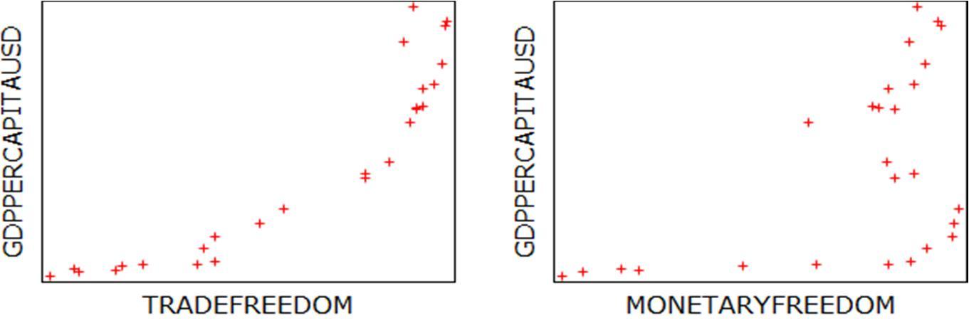
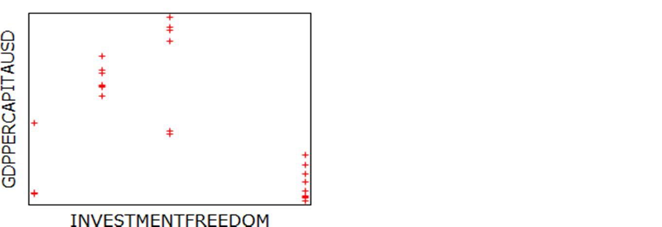
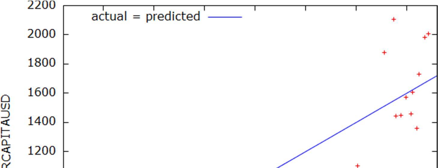
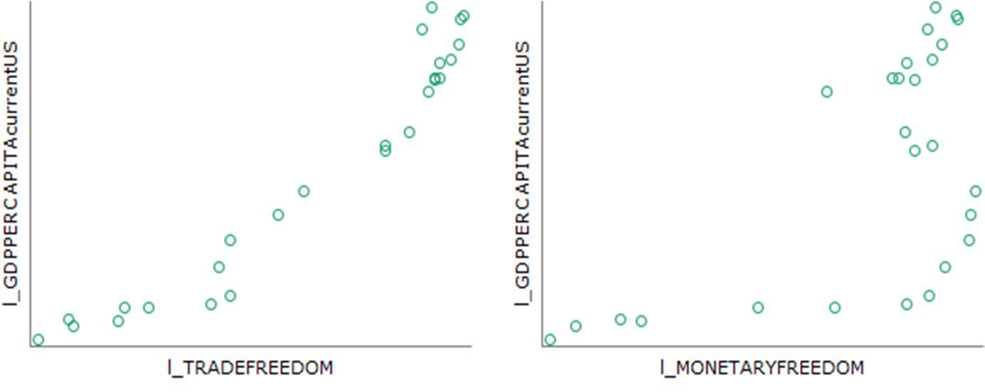
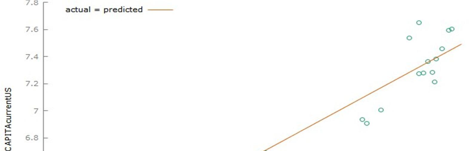
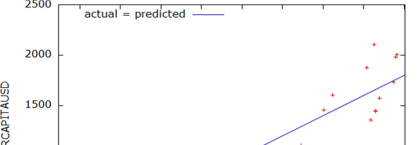
International Journal for Research in Applied Science & Engineering Technology (IJRASET) ISSN: 2321 9653; IC Value: 45.98; SJ Impact Factor: 7.538 Volume 10 Issue VII July 2022 Available at www.ijraset.com 5028©IJRASET: All Rights are Reserved | SJ Impact Factor 7.538 | ISRA Journal Impact Factor 7.894 | According to both t testing and p value testing, it is evident that β1, β2 and β3, are statistically significant and β4 is statistically insignificant at both 5% and 10% LOS Scatter Plot of X2, X3 and Y Actual vs. Fitted Graph

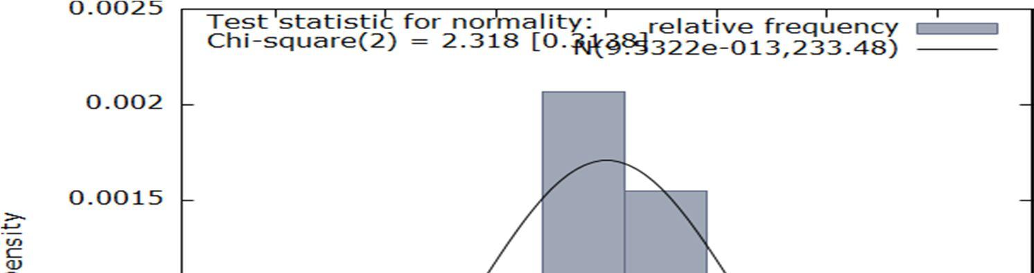
International Journal for Research in Applied Science & Engineering Technology (IJRASET) ISSN: 2321 9653; IC Value: 45.98; SJ Impact Factor: 7.538 Volume 10 Issue VII July 2022 Available at www.ijraset.com 5029©IJRASET: All Rights are Reserved | SJ Impact Factor 7.538 | ISRA Journal Impact Factor 7.894 |  ANOVA Table Analysis of Variance: Sum of squares df Mean square Regression 7.71893e+006 3 2.57298e+006 Residual 1.19932e+006 22 54514.8 Total 8.91826e+006 25 356730 R^2 = 7.71893e+006 / 8.91826e+006 = 0.865520 F(3, 22)= 2.57298e+006 / 54514.8 = 47.1978 [p value 9.42e 010] To check if this model is significant or not: Test Statistic = 47.1978 When α is 5% Critical Values: F0.05,3,22 = 3.05 Ho: R2 = 0Ha: R2 > 0 As Test Statistic value is greater than the Critical Value, it lies in the rejection region. Hence we reject Hoat 5% LOS. Model is significant at 5% LOS. When α is 10% Critical Values: F0.1,3,22 = 2.35 As Test Statistic value is greater than the Critical Value, it lies in the rejection region. Hence we reject Hoat 10% LOS. Model is significant at 10% LOS. Normality of Residual  Test for Normality of Residual Ho : ui is normally distributed Ha : ui is not normally distributed Chi square(2) = 2.318 with p value 0.31385 When α is 5% Since p value (0.31385) is greater than α (0.05), we fail to reject Ho at 5% LOS. This means that errorterms are normallydistributed at 5% LOS. When α is 10% Since p value (0.31385) is greater than α (0.1), we fail to reject Ho at 10% LOS. This means that errorterms are normally distributed at 10% LOS.

International Journal for Research in Applied Science & Engineering Technology (IJRASET) ISSN: 2321 9653; IC Value: 45.98; SJ Impact Factor: 7.538 Volume 10 Issue VII July 2022 Available at www.ijraset.com 5030©IJRASET: All Rights are Reserved | SJ Impact Factor 7.538 | ISRA Journal Impact Factor 7.894 | aux aux aux 0.05,3 Testing For Heteroscedasticity  BP Test Breusch Pagan test for heteroskedasticity OLS, using observations 1995 2020 (T = 26)Dependent variable: scaled uhat^2 coefficient std. error t ratio p value const 5.48372 4.90202 1.119 0.2753 TRADEFREEDOM 0.118478 0.0671869 1.763 0.0917 * MMONETARYFREEDO 0.0309425 0.0778167 0.3976 0.6947 OMINVESTMENTFREED 0.0142674 0.0425992 0.3349 0.7409 Explained sum of squares = 10.312Test statistic: LM = 5.156023, with p value= P(Chi square(3) > 5.156023) = 0.160722 When α is 5% Ho : R2 = 0 Ha : R2 > 0 As nR2 (Test statistic: LM = 5.156023) is less than χ 2 (7.8147), we fail to reject Ho at 5% LOS Thus there is no evidence of heteroscedasticity in the model at 5% LOS When α is 10% As nR2 aux (Test statistic: LM = 5.156023) is less than χ 20.1, 3 (6.2514), we fail toreject Ho at 10% LOS Thus there is no evidence of heteroscedasticity in the model at 10% LOS  White’s Test White's test for heteroskedasticity OLS, using observations 1995 2020 (T = 26) Dependent variable: uhat^2 coefficient std. error t ratio p value const −1.80930e+06 7.11417e+06 0.2543 0.8025 TRADEFREEDOM 18305.1 154558 0.1184 0.9072 MONETARYFREEDOM 42002.6 232144 0.1809 0.8587 INVESTMENTFREEDOM −15703.4 97645.4 0.1608 0.8742 sq_TRADEFREEDOM −1021.17 1485.88 0.6873 0.5018 X2_X3 1190.19 2233.87 0.5328 0.6015 X2_X4 1056.79 1025.39 1.031 0.3180 sq_MONETARYFREED~ −794.184 1975.38 0.4020 0.6930 X3_X4 −386.702 1051.25 0.3678 0.7178 sq_INVESTMENTFRE~ −290.749 945.516 0.3075 0.7624 Unadjusted R squared = 0.428191 Test statistic: TR^2 = 11.132958, with p value= P(Chi square(9) > 11.132958)= 0.266705

International Journal for Research in Applied Science & Engineering Technology (IJRASET) ISSN: 2321 9653; IC Value: 45.98; SJ Impact Factor: 7.538 Volume 10 Issue VII July 2022 Available at www.ijraset.com 5031©IJRASET: All Rights are Reserved | SJ Impact Factor 7.538 | ISRA Journal Impact Factor 7.894 | aux aux aux 0.05,9 aux 0.05,1 aux 0.1,1 ’ Hence both BP and White’s Test show no heteroscedasticity in the model at 5% & 10% LOS BG Test shows evidence of autocorrelation in the model at 5% and 10% LOS. This may be a possible reason for nonconformity of b4 with its apriori expectation When α is 5% Ho : R2 = 0 Ha : R2 > 0 As nR2 (Test statistic: TR2 = 11.132958) is less than χ2 (16.919), we fail to reject Ho at 5% LOS Thus there is no evidence of heteroscedasticity in the model at 5% LOS When α is 10% As nR2 aux (Test statistic: TR2 = 11.132958) is less than χ 20.1, 9 (14.6837), we fail to reject Ho at 10% LOS Thus there is no evidence of heteroscedasticity in the model at 10% LOS  BG Test Testing for Autocorrelation Breusch Godfrey test for first order autocorrelationOLS, using observations 1995 2020 (T = 26) Dependent variable: uhat coefficient std. error t ratio p value const 171.967 475.196 0.3619 0.7211 TRADEFREEDOM 2.79461 6.51703 0.4288 0.6724 MONETARYFREEDOM 3.34293 7.54917 0.4428 0.6624 MINVESTMENTFREEDO 2.69740 4.14363 0.6510 0.5221 uhat_1 0.883187 0.134372 6.573 1.65e 06 *** UnadjustedR squared = 0.672899 Test statistic: LMF = 43.200294, with p value = P(F(1,21) > 43.2003) = 1.65e 006 When α is 5% Ho: There is no autocorrelation in the modelHa: There is autocorrelation in the model As (n p)R2 (Test statistic:LMF = 43.200294) is greater than χ 2 (3.8415), we reject Ho at 5% LOS Thus there is evidence of autocorrelation in the model at 5% LOS When α is 10% As (n p)R2 (Test statistic:LMF = 43.200294) is greater than χ 2 (2.7055), we reject Ho at 5% LOS Thus there is evidence of autocorrelation in the model at 10% LOS  Durbin Watson Test Durbin Watson statistic 0.358754 Ho : No positive auto correlation H0 : No negative auto correlation

International Journal for Research in Applied Science & Engineering Technology (IJRASET) ISSN: 2321 9653; IC Value: 45.98; SJ Impact Factor: 7.538 Volume 10 Issue VII July 2022 Available at www.ijraset.com 5032©IJRASET: All Rights are Reserved | SJ Impact Factor 7.538 | ISRA Journal Impact Factor 7.894 | This could be a possible reason for non-conformity of estimated coeffecient (β4) with our apriori expectations. Since none of the VIF’s are > 10, there is no evidence of Multicollinearity in the estimated model At alpha = 0.05, n=26, k ’ = 3 , dL = 1.143, du = 1.652 As, 0 < Sample calculated d test statistic = 0.358754 < dL ,therefore we reject H0 i.e. there is evidenceof positive auto correlation. Testing for Multicollinearity Variance Inflation Factors Minimum possible value = 1.0 Values > 10.0 may indicate a collinearityproblem TRADEFREEDOM 2.562 MONETARYFREEDOM 2.103 INVESTMENTFREEDOM 1.334 VIF(j) = 1/(1 R(j)^2), where R(j) is themultiple correlation coefficientbetween variable j and the other independent variables  Correlation Matrix Correlation coefficients, using the observations 1995 20205% critical value (two tailed) = 0.3882 for n = 26 AUSDTGDPPERCAPI MOTRADEFREED EDOMREMONETARYF REEDOMINVESTMENTF 1.0000 0.9115 0.5340 0.4010 AUSDGDPPERCAPIT 1.0000 0.7173 0.4848 MOTRADEFREED 1.0000 0.2606 EDOMEMONETARYFR 1.0000 REEDOMINVESTMENTF  Confidence Intervals for Coefficients t(22, 0.025) = 2.074 Variable Coefficient 95 confidence interval const 3998.06 ( 5679.00, 2317.11) TRADEFREEDOM 101.152 (78.1130, 124.191) MONETARYFREEDOM 29.6823 ( 56.3663, 2.99831) INVESTMENTFREEDOM 6.49479 ( 8.11283, 21.1024)

One Dependent And Three Explanatory VariablesFunctional Forms: Double Log Model  Interpretation Effect of log Trade freedom, log monetary freedom and log investment freedom on log of GDPper capita Y: GDP per capita (billion USD)X2i :Trade Freedom (index) X3i : Monetary Freedom (index) X4i : Investment Freedom (index) lnY = β1 + β2 ln X2i + β3ln X3i + β4 lnX4i + ui (where β2, β3, β4 are the parameters and ui is the random error term)

Linear Model

β2 is the elasticity of GDP per capita with respect to trade freedom, holding other variablesconstant.

β4 is the elasticity of GDP per capita with respect to investment freedom, holding other variablesconstant.

Apriori expectations of β3 is positive, an increase in ln monetary freedom leads to price stability,thus encouraging savings and investment, hence leading to a higher ln per capita GDP.

Apriori expectations of β4 is positive because an increase in the ln investment freedom, higherwould be the investment in the country by residents and foreigners, hence greater would be lnGDP per capita.

International Journal for Research in Applied Science & Engineering Technology (IJRASET) ISSN: 2321 9653; IC Value: 45.98; SJ Impact Factor: 7.538 Volume 10 Issue VII July 2022 Available at www.ijraset.com 5033©IJRASET: All Rights are Reserved | SJ Impact Factor 7.538 | ISRA Journal Impact Factor 7.894 | r ur r ur The restricted model has both lower Schwartz criterion and Akaike criterion than the unrestrictedmodel, therefore, we can conclude that restricted model is better.  Extension Restricted vs. Unrestricted Restricted Model: Y = β1 +β2X2i + ui (R2 = 0.830801) Unrestricted Model: Y = β1 +β2X2i + β3X3i + β4X4i + ui (R2 = 0.865520) (m is number of restrictions imposed = 2) Ho: β3 = β4 = 0 Ha: At least one of either β3 orβ4 ≠ 0 fcalc = (R2 ur R2 ) / m = 2.845(1 R2 ) / (n k) When α is 5%: As fcalc is less than fcrit 0.05, 2, 22 (3.44), we fail toreject Ho at 5% LOS Restrictions imposed are valid at 5% LOS. When α is 10%: As fcalc is greater than fcrit 0.1, 2, 22 (2.56), we reject Ho at 5% LOSRestrictions imposed are not valid at 10% LOS.

β 1 is the mean value of ln GDP per capita when Trade, Monetary and Investment Freedom are all1.

 Apriori Expectations of Partial Coefficients

β3 is the elasticity of GDP per capita with respect to monetary freedom, holding other variablesconstant.

Estimated equation Ln Y ^ (Y Hat) = b1 + b2 ln X2i + b3ln X3i, + b4 ln X4i, (where b1, b2, b3 and b4 are estimators of β1, β2, β3 and β4 respectively).

Here, apriori expectations of β2 are positive, an increase in ln trade freedom results in corresponding increase in ln GDP per capita, due to higher trade in goods and services with othercountries.

R2 value (overall goodness of fit measure) of 0.947350 means that 94.73% of total variation inthe ln GDP per capita around its mean value is explained by ln trade freedom, ln monetary freedom and ln investment freedom together.

 For β 3: As the t ratio or tcalc = 2.973 is less than tcritical,0.05,22 = 1.717, we reject Ho at 5%level of significance (or data is statisticallysignificant at 5% LOS).

 t Testing of b2 and b3 Ho: β2 = 0; β3=0; β4 = 0Ha: β2 > 0; β3 > 0; β4 >0 Assuming that b1, b2, b3 and b4 follow approx. normal distribution with mean β1, β2, β3 and β4respectively: At 5% level of significance

International Journal for Research in Applied Science & Engineering Technology (IJRASET) ISSN: 2321 9653; IC Value: 45.98; SJ Impact Factor: 7.538 Volume 10 Issue VII July 2022 Available at www.ijraset.com 5034©IJRASET: All Rights are Reserved | SJ Impact Factor 7.538 | ISRA Journal Impact Factor 7.894 | Y ^ (Y Hat) = 16.4788 + 7.06879X2i 1.74612X3i + 0.24161X4i  Running the Regression by OLS method Model 1: OLS, using observations 1995 2020 (T = 26)Dependent variable: l_GDPPERCAPITAcurrentUS Coefficient Std. Error t ratio p value Const 16.4788 2.03094 8.114 <0.0001 *** l_TRADEFREEDOM 7.06879 0.480212 14.72 <0.0001 *** OMl_MONETARYFREED 1.74612 0.587367 2.973 0.0070 *** OMDl_INVESTMENTFREE 0.240161 0.176585 1.360 0.1876 Mean dependent var 6.804483 S.D. dependent var 0.616540 Sum squared resid 0.500334 S.E. of regression 0.150806 R squared 0.947350 Adjusted R squared 0.940171 F(3, 22) 131.9516 P value(F) 3.25e 14 Ln likelihood 14.46507 Akaike criterion 20.93015 Schwarz criterion 15.89776 Hannan Quinn 19.48100 Rho 0.643499 Durbin Watson 0.742500 According to the regression run by OLS method, it can be seen that the estimated coefficients are:b1 = −16.4788 b2 = 7.06879 b3 = −1.74612 b4= 0.240161 b1, Theoretically, when trade freedom, monetary freedom and investment freedom are all 1, then the estimated mean value of ln GDP per capita would be −16.4788 per USD. In the current, it is insignificant as India’s Trade freedom, monetary freedom, and investment freedom have not beenzero in the last 25 years. b2 is positive implying that an increase in the trade freedom will lead to an increase in per capita GDP. In other words, an increase in India’s trade freedom by1% leads to an increase in estimatedmean GDP per capita by7.06879%, holding other factors constant. b3 is negative implying that an increase in the monetary freedom will lead to a decrease in per capita GDP. In other words, an increase in India’s monetary freedom by 1% will lead to a decrease in estimated mean GDP per capita by 1.74612%, holding other factors constant. But thisdoes not conform to our apriori expectations of b3 possibly because of some CLRM assumptions not being satisfied. b4 is positive implying that an increase in the investment freedom will lead to an increase in percapita GDP. In other words, an increase in India’s investment freedom by 1%, leads to an increase in estimated mean GDP per capita by 0.24161 %, holding other factors constant.

 For β2: As the t ratio or tcal = 14.72 is greater than tcritical,0.05,22 = 1.717, we reject Ho at 5%level of significance (or data is statisticallysignificant at 5% LOS).

 Comparing p value and α When α is 5%  β2 is statistically significant as its p value 7.17e 013 (1.62×10 5) is less than 5% α or(1.62×10 5) ≤ 0.05.

According to both t testing and p-value testing, it is evident that β1, β2 and β3, are statistically significant and β4 is statistically insignificant at both 5% and 10% LOS

 For β 4: As the t ratio or tcalc = 1.360 is greater than tcritical,0.05,22 = 1.717, we fail to rejectHo at 5% level of significance (or data is statisticallyinsignificant at 5% LOS). At 10% level of significance

 β4 is statistically insignificant as its p value 0.1876 is greater than 5% α or 0.1876 ≥ 0.05. When α is 10%  β2 is statistically significant as its p value 7.17e 013 (1.62×10 5) is less than 10% α or1.62×10 5≤ 0.1.

 For β 4: As the t ratio or tcalc = 1.360 is greater than tcritical,0.10,22 = 1.321, we reject Ho at10% level of significance (or data is statisticallysignificant at 10% LOS).

 β3 is statistically significant as its p value 0.0070 is less than 5% α or 0.0070 ≤ 0.05.

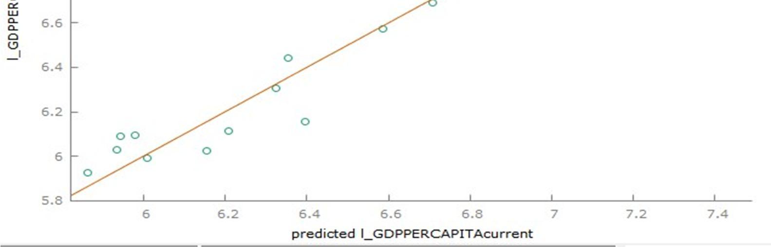
 β3 is statisticallysignificant as its p value 0.0070 is less than 10% α or 0.0070 ≤ 0.1  β4 is statisticallyinsignificant as its p value 0.1876 is greater than 10% α or 0.1876 > 0.1 Scatter Plot of X2, X3 and Y

 For β 3: As the t ratio or tcalc = 2.973 is less than tcritical,0.10,22 = 1.321, we reject Ho at 10%level of significance (or data is statisticallysignificant at 10% LOS).

 For β2: As the t ratio or tcal = 14.72 is greater than tcritical,0.10,22 = 1.321, we reject Ho at10% level of significance (or data is statisticallysignificant at 10% LOS).

International Journal for Research in Applied Science & Engineering Technology (IJRASET) ISSN: 2321 9653; IC Value: 45.98; SJ Impact Factor: 7.538 Volume 10 Issue VII July 2022 Available at www.ijraset.com 5035©IJRASET: All Rights are Reserved | SJ Impact Factor 7.538 | ISRA Journal Impact Factor 7.894 |

International Journal for Research in Applied Science & Engineering Technology (IJRASET) ISSN: 2321 9653; IC Value: 45.98; SJ Impact Factor: 7.538 Volume 10 Issue VII July 2022 Available at www.ijraset.com 5036©IJRASET: All Rights are Reserved | SJ Impact Factor 7.538 | ISRA Journal Impact Factor 7.894 | Actual vs. Fitted  Anova Table Analysis of Variance: Sum of squares df Mean square Regression 9.00272 3 3.00091 Residual 0.500334 22 0.0227425 Total 9.50305 25 0.380122 R^2 = 9.00272 / 9.50305 = 0.947350 F(3, 22)= 3.00091 / 0.0227425 = 131.952 [p value 3.25e 014] To check if themodel is significant or not Test Statistic= f=131.952 When α is 5% Critical Values: F0.05,3,22 = 3.05  H0 :R2=0Ha :R2>0 As Test Statistic value is greater than the Critical Value, it lies in the rejection region. Hence we reject Hoat 5% LOS. Model is significant at 5% LOS. When α is 10% Critical Values: F0.1,3,22 = 2.35 As Test Statistic value is greater than the Critical Value, it lies in the rejection region. Hence we reject Hoat 10% LOS. Model is significant at 10% LOS.

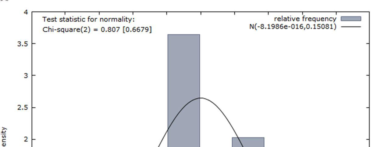
International Journal for Research in Applied Science & Engineering Technology (IJRASET) ISSN: 2321 9653; IC Value: 45.98; SJ Impact Factor: 7.538 Volume 10 Issue VII July 2022 Available at www.ijraset.com 5037©IJRASET: All Rights are Reserved | SJ Impact Factor 7.538 | ISRA Journal Impact Factor 7.894 | Normalityof Residual  Test for Normality of Residual: Ho : ui is normally distributed Ha : ui is notnormally distributed Chi square (2) = 0.807 with p value 0.6679 When α is 5% Since p value (0.6679) is greater than α (0.05), we fail to reject Ho at 5% LOS. This means that errorterms are normallydistributed at 5% LOS. When α is 10% Since p value (0.6679) is greater than α (0.1), we fail to reject Ho at 10% LOS. This means that errorterms are normallydistributed at 10% LOS. Testing for Heteroscedasticity It is possible that are model is suffering from heteroskedasticityas there are few statistical insignificantratios, as a result t test are unreliable.  Breush Pagan Test Breusch Pagan test for heteroskedasticity OLS, using observations 1995 2020 (T = 26) Dependent variable: scaled uhat^2coefficient std. error t ratio p value const −16.5880 18.3590 0.9035 0.3760 l_TRADEFREEDOM 3.37788 4.34097 0.7781 0.4448 l_MONETARYFREEDOM 0.272133 5.30961 0.05125 0.9596 l_INVESTMENTFREE~ 0.582898 1.59627 0.3652 0.7185 Explained sum of squares = 2.63358 Test statistic: LM = 1.316791, with p value= P(Chi square(3)> 1.316791) = 0.725150

International Journal for Research in Applied Science & Engineering Technology (IJRASET) ISSN: 2321 9653; IC Value: 45.98; SJ Impact Factor: 7.538 Volume 10 Issue VII July 2022 Available at www.ijraset.com 5038©IJRASET: All Rights are Reserved | SJ Impact Factor 7.538 | ISRA Journal Impact Factor 7.894 | aux aux aux aux aux 0.05,9 Hence both BP and White’s Test show no heteroscedasticity in the model at 5% & 10% LOS When α is 5% H0: R2 =0 Ha: R2 >0 As nR2 aux (Test statistic: LM = 1.316791) is less than χ 20.05, 3 (7.8147), we fail to reject Ho at 5% LOS Thus there is no evidence of heteroscedasticity in the model at 5% LOSWhen α is 10% As nR2 aux (Test statistic: LM = 1.316791) is less than χ 20.1, 3 (6.2514), we fail toreject Ho at 10% LOS Thus there is no evidence of heteroscedasticity in the model at 10% LOS  White’s General Test White's test for heteroskedasticity OLS, using observations 1995 2020 (T = 26) Dependent variable: uhat^2 coefficient std. error t ratio p value const 47.7713 48.0176 0.9949 0.3346 l_TRADEFREEDOM 1.80242 18.4971 0.09744 0.9236 OMl_MONETARYFREED 25.2109 26.4965 0.9515 0.3555 l_INVESTMENTFREE 1.18796 6.11119 0.1944 0.8483 Msq_l_TRADEFREEDO 1.53762 3.02609 0.5081 0.6183 X2_X3 2.66111 4.54450 0.5856 0.5663 X2_X4 0.957254 1.03397 0.9258 0.3683 ~sq_l_MONETARYFRE 4.01616 3.86481 1.039 0.3142 X3_X4 0.639635 1.21299 0.5273 0.6052 sq_l_INVESTMENTF~ 0.000732506 0.616480 0.001188 0.9991 Unadjusted R squared = 0.297537 Test statistic: TR^2 = 7.735972, with p value= P(Chi square(9) > 7.735972) = 0.560957 When α is 5% H0: R2 =0 Ha: R2 >0 As nR2 (Test statistic: TR2 = 7.73597) is less than χ 2 (16.919), we fail to reject Ho at 5% LOS Thus there is no evidence of heteroscedasticity in the model at 5% LOS When α is 10% As nR2 aux (Test statistic: TR2 = 7.73597) is less than χ 20.1, 9 (14.6837), we fail to reject Ho at 10% LOS Thus there is no evidence of heteroscedasticity in the model at 10% LOS

’ =

< Sample calculated

International Journal for Research in Applied Science & Engineering Technology (IJRASET) ISSN: 2321 9653; IC Value: 45.98; SJ Impact Factor: 7.538 Volume 10 Issue VII July 2022 Available at www.ijraset.com 5039©IJRASET: All Rights are Reserved | SJ Impact Factor 7.538 | ISRA Journal Impact Factor 7.894 | aux 0.05,1 aux 0.1,1 BG Test shows evidence of autocorrelation in the model at 5% and 10% LOS. This may be a possible reason for nonconformity of b4 with its apriori expectation This could be a possible reason for non conformity of estimated coeffecient (b4) with our apriori expectations. Testing For Autocorrelation There is possibilitythat the model is suffering from autocorrelation.  BG Test Breusch Godfrey test for first order autocorrelationOLS, using observations 1995 2020 (T = 26) Dependent variable: uhat coefficient std. error t ratio p value const 0.0977565 1.65504 0.05907 0.9535 l_TRADEFREEDOM 0.0119301 0.391289 0.03049 0.9760 OMl_MONETARYFREED 0.00190859 0.478584 0.003988 0.9969 ~l_INVESTMENTFREE 0.0406852 0.144353 0.2818 0.7808 uhat_1 0.653370 0.187537 3.484 0.0022 *** Unadjusted R squared = 0.366286 Test statistic: LMF = 12.137973, with p value = P(F(1,21) > 12.138) = 0.00221  Ho: There is no autocorrelation in the modelHa: There is autocorrelation in the model When α is 5% As (n p)R2 (Test statistic:LMF = 12.137973) is greater than χ 2 (3.8415), we reject Ho at 5% LOS Thus there is evidence of autocorrelation in the model at 5% LOS When α is 10% As (n p)R2 (Test statistic:LMF = 12.137973) is greater than χ 2 (2.7055), we reject Ho at 5% LOS

=

, dL = 1.143,

= 0.05, n=26,

Thus there is evidence of autocorrelation in the model at 10% Watson Test Durbin Watson statistic = 0.7425p value 1.05318e No positive auto correlation H0’ No negative auto correlation At alpha k 3 du 0 d statistic < therefore reject H0 there evidence

005 Ho :

test

= 0.7425

is

= 1.652 As ,

we

:

LOS  Durbin

i.e.

ofpositive auto correlation.

dL ,

International Journal for Research in Applied Science & Engineering Technology (IJRASET) ISSN: 2321 9653; IC Value: 45.98; SJ Impact Factor: 7.538 Volume 10 Issue VII July 2022 Available at www.ijraset.com 5040©IJRASET: All Rights are Reserved | SJ Impact Factor 7.538 | ISRA Journal Impact Factor 7.894 | Since none of the VIF’s are > 10, there is no evidence of Multicollinearity in the estimated model Testing For Multicollinearity Variance Inflation Factors Minimum possible value = 1.0 Values > 10.0 may indicate a collinearityproblem l_TRADEFREEDOM 2.569 l_MONETARYFREEDOM 2.242 l_INVESTMENTFREEDOM 1.239 VIF(j) = 1/(1 R(j)^2), where R(j) is themultiple correlation coefficientbetween variable j and the other independent variables  Coefficient Covariance Matrix Const l_TRADEFREEDOM l_MONETARYFREEDOM l_INVESTMENTFREEDOM 4.12471 0.217126 0.575486 0.201566 const 0.230603 0.203932 0.0313437 l_TRADEFREEDOM 0.345000 0.0107057 l_MONETARYFREEDOM 0.0311822 l_INVESTMENTFREEDOM  Confidence Intervals for Coefficients t(22, 0.025) = 2.074 Variable Coefficient 95 confidence interval const 16.4788 ( 20.6907, 12.2668) l_TRADEFREEDOM 7.06879 (6.07289, 8.06469) Ml_MONETARYFREEDO 1.74612 ( 2.96424, 0.527991) Ml_INVESTMENTFREEDO 0.240161 ( 0.126054, 0.606375) Dummy Model One Dependent, Two Explanatory Variables And Two DummyVariables  Interpretation Effect of India’s Trade Freedom, MonetaryFreedom and level of Foreign Direct Investment onGDP per capita (USD) along with effect of Investment Freedom on GDP per capita (USD) by enacting structural break in data set for two different periods :1995 2007 and 2007 2020.Y:GDP per capita (billion USD) X2i : India’s Trade Freedom (index) X3i : India’s Investment Freedom (index) D1i = 1 if FDI (% of GDP) is ≥ 2%0 if FDI (% of GDP) is < 2% D2i = 1 for the time period 1995 20070 for thetime period 2008 2020

 Differential Slope Coefficient: β4 = E(Y^|X=1, D1i = 0 and D2i = 1), when India’s investment freedom increases by 1 unit, the estimated mean GDP per capita for the period 1995 2007 is higher by β4 units as compared to the estimated mean GDP per capita for the period 2007 2020,keeping everything else constant. Y ^ (Y Hat) = b1 + b2X2i + b3D1i,+ b4D2iX3i β1, β2, 3, b2 is positive implying that an increase in India’s trade freedom by 1 unit, leads to an increase inestimated mean GDP per capita by 70.2234 billion USD. b3 = −274.899 billion USDis the difference between the mean GDP per capita when FDI(% ofGDP) is greater than 2% as compared to the reference category, keeping everything constant. b4, when India’s investment freedom increases by 1 unit, the estimated mean GDP per capita for the period 1995 2007 is less by 5.43497 billion USD as compared to the estimated mean GDP percapita for the period 2007 2020, keeping everything else constant. But this does not confirm to our apriori expectations of b2 possibly because of some CLRM assumptions not being satisfied.

R2 value (overall goodness of fit measure) of 0.886625 means that 88.6625 % of total variationin estimated GDP per capita around its mean value is explained by Trade freedom, Investment freedom and FDI(% of GDP)

 Reference category: β1 = E(Y^|X=0, D1i = 0 and D2i = 0) The mean GDP per capita for the period 2008 2020 when India’s trade freedom and investment freedom are zero and FDI(% ofGDP) is < 2%.

 Differential Intercept Coefficient: β3 = E(Y^|X=0, D1i = 1 and D2i = 0) is the difference betweenthe mean GDP per capita when FDI(% of GDP) is greater than 2% as compared to the reference category, keeping everything constant.

β

(where b1, b2, b3, b4 and b5 are estimators of

International Journal for Research in Applied Science & Engineering Technology (IJRASET) ISSN: 2321 9653; IC Value: 45.98; SJ Impact Factor: 7.538 Volume 10 Issue VII July 2022 Available at www.ijraset.com 5041©IJRASET: All Rights are Reserved | SJ Impact Factor 7.538 | ISRA Journal Impact Factor 7.894 |

Y ^ (Y Hat) = 3574.08+ 70.2234X2i 274.899 D1i, 5.43487D2iX3i Y = β1 +β2X2i + β3D1i + β4D2iX3i + ui (where β2, β3, β4 are the parameters and ui is the random error term)

 Slope Coefficient : β2 = E(Y^|X=1,D1i = 0 and D2i = 0 ) is the partial slope coefficients of meanGDP per capita w.r.t Trade Freedom.

β4 and β5 respectively).  Running the Regression by OLS method Model 2: OLS, using observations 1995 2020 (T = 26)Dependent variable: GDPPERCAPITAUSD Coefficient Std. Error t ratio p value Const 3574.08 956.585 3.736 0.0011 *** TRADEFREEDOM 70.2234 13.0030 5.401 <0.0001 *** DummyFDI 274.899 107.342 2.561 0.0178 ** DiInvFree 5.43497 3.57790 1.519 0.1430 Mean dependent var 1070.181 S.D. dependent var 597.2691 Sum squared resid 1011109 S.E. of regression 214.3816 R squared 0.886625 Adjusted R squared 0.871165 F(3, 22) 57.34871 P value(F) 1.46e 10 Ln likelihood 174.2824 Akaike criterion 356.5648 Schwarz criterion 361.5972 Hannan Quinn 358.0139 Rho 0.638151 Durbin Watson 0.686341 According to the regression run by OLS method, it can be seen that the estimated coefficients are:b1 = −3574.08 b2 = 70.2234 b3 = −274.899 b4 = −5.43497 b1 in the current model is insignificant as India’s trade freedom, investment freedom and FDI(%of GDP) have not been zero in the last 26 years.

International Journal for Research in Applied Science & Engineering Technology (IJRASET) ISSN: 2321 9653; IC Value: 45.98; SJ Impact Factor: 7.538 Volume 10 Issue VII July 2022 Available at www.ijraset.com 5042©IJRASET: All Rights are Reserved | SJ Impact Factor 7.538 | ISRA Journal Impact Factor 7.894 |

 For β4: As the t ratio or tcalc = −1.519 is less than the tcritical,0.05,22 = 1.717, we fail to rejectHo at 5% level of significance (or β4 is statistically insignificant at 5% level of significance). At 10% level of significance

 For β 2: As the t ratio or tcalc = 5.401 is greater than the tcritical,0.05,22 = 1.321, we reject Ho at5% level of significance (or β2 is statisticallysignificant at 5% level of significance).

Accordint to p value, it is evident that β1, β2 and β3 are statistically significant and β4 is statistically insignificant at both 5% and 10% LOS.

 For β 4: As the t ratio or tcalc = −1.519 is more than the tcritical,0.05,22 = 1.321, we reject Ho at5% level of significance (or β4 is statisticallysignificant at 5% level of significance).

 t Testing of b2 and b3

 For β3: As the t ratio or tcalc = −2.561 is less than the tcritical,0.05,22 = 1.321, we reject Ho at5% level of significance (or β3 is statisticallysignificant at 5% level of significance).

 β2 is statisticallysignificant as its p value <0.0001 is less than 5% α or <0.0001 ≤ 0.05  β3 is statisticallysignificant as its p value 0.0178 is less than 5% α or (0.0178) ≤ 0.05  β4 is statistically insignificant as its p value 0.1430 is greater than 5% α or (0.1430) >0.05 When α is 10%  β1 is statistically significant as its p value 0.0011 is less than 10% α or(0.0011) ≤ 0.1.  β2 is statisticallysignificant as its p value <0.0001 is less than 10% α or <0.0001 ≤ 0.1.

 β3 is statisticallysignificant as its p value 0.0178 is less than 10% α or (0.0178) ≤ 0.1  β4 is statistically insignificant as its p value 0.1430 is greater than 10% α or (0.1430) >0.1

According to t testing, it is evident that β1, β2 and β3, are statistically significant at both 5% and 10% LOS and β4 is statistically insignificant at 5% and significant at 10%

Assuming that b1, b2 and b3 follow approx. normal distribution with mean β1, β2 and β3respectively: At 5 % level of significance

 Comparing p value and α When α is 5%  β1 is statistically significant as its p value 0.0011 is less than 5% α or(0.0011) ≤ 0.05.

 For β2: As the t ratio or tcalc = 5.401 is greater than the tcritical,0.05,22 = 1.717, we reject Ho at5% level of significance (or β2 is statisticallysignificant at 5% level of significance).

 For β3: As the t ratio or tcalc = −2.561 is less than the tcritical,0.05,22 = 1.717, we reject Ho at5% level of significance (or β3 is statisticallysignificant at 5% level of significance).

International Journal for Research in Applied Science & Engineering Technology (IJRASET) ISSN: 2321 9653; IC Value: 45.98; SJ Impact Factor: 7.538 Volume 10 Issue VII July 2022 Available at www.ijraset.com 5043©IJRASET: All Rights are Reserved | SJ Impact Factor 7.538 | ISRA Journal Impact Factor 7.894 | Scatter Plot of X2, X3 and Y Actual vs. Fitted Graph

International Journal for Research in Applied Science & Engineering Technology (IJRASET) ISSN: 2321 9653; IC Value: 45.98; SJ Impact Factor: 7.538 Volume 10 Issue VII July 2022 Available at www.ijraset.com 5044©IJRASET: All Rights are Reserved | SJ Impact Factor 7.538 | ISRA Journal Impact Factor 7.894 |  Anova Table Analysis of Variance: Sum of squares df Mean square Regression 7.90715e+006 3 2.63572e+006 Residual 1.01111e+006 22 45959.5 Total 8.91826e+006 25 356730 R^2 = 7.90715e+006 / 8.91826e+006 = 0.886625 F(3, 22) = 2.63572e+006 / 45959.5 = 57.3487 [p value 1.46e 010] To check if this model is significant or not: Test Statistic = 57.3487 When α is 5% Critical Values: F0.05,3,22 = 3.05  Ho: R2 = 0Ha: R2 > 0 As Test Statistic value is greater than the Critical Value, it lies in the rejection region. Hence we reject Hoat 5% LOS. Model is significant at 5% LOS. When α is 10% Critical Values: F0.1,3,22 = 2.35 As Test Statistic value is greater than the Critical Value, it lies in the rejection region. Hence we reject Hoat 10% LOS. Model is significant at 10% LOS. Normality of Residual

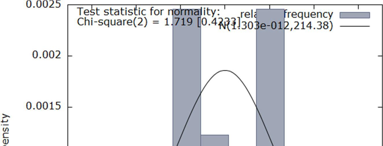
International Journal for Research in Applied Science & Engineering Technology (IJRASET) ISSN: 2321 9653; IC Value: 45.98; SJ Impact Factor: 7.538 Volume 10 Issue VII July 2022 Available at www.ijraset.com 5045©IJRASET: All Rights are Reserved | SJ Impact Factor 7.538 | ISRA Journal Impact Factor 7.894 | aux aux aux 0.05,3  Test for Normality of Residual: Ho : ui is normally distributed Ha : ui is not normally distributed Chi square(2) = 1.719 with p value 0.4233 When α is 5% Since p value (0.4233) is greater than α (0.05), we fail to reject Ho at 5% LOS. This means that errorterms are normallydistributed at 5% LOS. When α is 10% Since p value (0.4233) is greater than α (0.1), we fail to reject Ho at 10% LOS. This means that errorterms are normallydistributed at 10% LOS. Testing for Heteroscedasticity It is possible that are model is suffering from heteroskedasticityas there are few statistical insignificantratios, as a result t test are unreliable.  Breusch Pagan Test Breusch Pagan test for heteroskedasticity OLS, using observations 1995 2020 (T = 26)Dependent variable: scaled uhat^2 coefficient std. error t ratio p value const 1.75129 4.71488 0.3714 0.7139 MTRADEFREEDO 0.00295394 0.0640899 0.04609 0.9637 DummyFDI 0.721107 0.529072 1.363 0.1867 DiInvFree 0.0171132 0.0176350 0.9704 0.3424 Explained sum of squares = 5.14258Test statistic: LM = 2.571289, with p value = P(Chi square(3) > 2.571289) = 0.462545Ho : R2 = 0 Ha : R2 > 0 When α is 5% As nR2 (Test statistic: LM = 2.571289) is less than χ 2 (7.8147), we fail to reject Ho at 5% LOS Thus there is no evidence of heteroscedasticity in the model at 5% LOS When α is 10% As nR2 aux (Test statistic: LM = 2.571289 ) is less than χ20.1, 3 (6.2514), we fail toreject Ho at 10% LOS Thus there is no evidence of heteroscedasticity in the model at 10% LOS  White’s Test White's test for heteroskedasticity OLS, using observations 1995 2020 (T = 26) Dependent variable: uhat^2 coefficient std. error t ratio p value const 5.19205e+06 6.92426e+06 0.7498 0.4636 TRADEFREEDOM 155024 187131 0.8284 0.4189 DummyFDI 649578 1.74311e+06 0.3727 0.7140 DiInvFree 18983.1 56614.6 0.3353 0.7415 Msq_TRADEFREEDO 1133.10 1275.77 0.8882 0.3868 X2_X3 8157.61 23388.7 0.3488 0.7315

is

we

Thus there is evidence of autocorrelation in the model at 5%

in the

As (n p)R2

LOS

LOS

International Journal for Research in Applied Science & Engineering Technology (IJRASET) ISSN: 2321 9653; IC Value: 45.98; SJ Impact Factor: 7.538 Volume 10 Issue VII July 2022 Available at www.ijraset.com 5046©IJRASET: All Rights are Reserved | SJ Impact Factor 7.538 | ISRA Journal Impact Factor 7.894 | aux aux aux 0.05,9 aux 0.05,1 Hence both BP and White’s Test show no heteroscedasticity in the model at 5% & 10% LOS BG Test shows evidence of autocorrelation in the model at 5% and 10% LOS. This may be a possible reason for nonconformity of b4 with its apriori expectation X2_X4 324.652 692.187 0.4690 0.6450 X3_X4 2737.37 3394.07 0.8065 0.4311 sq_DiInvFree 13.6848 187.439 0.07301 0.9427 Unadjusted R squared= 0.252721Test statistic: TR^2 = 6.570747, with p value= P(Chi square(8) > 6.570747) = 0.583571 Ho : R2 = 0 Ha : R2 > 0 When α is 5% As nR2 (Test statistic: TR2 = 6.570747) is less than χ2 (16.919), we fail to reject Ho at 5% LOS Thus there is no evidence of heteroscedasticity in the model at 5% LOS When α is 10% As nR2 aux (Test statistic: TR2 = 6.570747) is less than χ 20.1, 9 (14.6837), we fail to reject Ho at 10% LOS Thus there is no evidence of heteroscedasticity in the model at 10% LOS Testing for Autocorrelation  BG Test Breusch Godfrey test for first order autocorrelationOLS, using observations 1995 2020 (T = 26) Dependent variable: uhat coefficient std. error t ratio p value const −371.815 757.418 0.4909 0.6286 TRADEFREEDOM 4.78096 10.2868 0.4648 0.6469 DummyFDI 63.9707 85.9299 0.7445 0.4649 DiInvFree 1.57927 2.83968 0.5561 0.5840 uhat_1 0.691260 0.180436 3.831 0.0010 *** Unadjusted R squared = 0.411385 Test statistic: LMF = 14.676996, with p value= P(F(1,21) > 14.677) = 0.000972 Alternative statistic:TR^2 = 10.696021, with p value = P(Chi square(1) > 10.696) = 0.00107Ljung Box Q' = 10.3135, with p value = P(Chi square(1) > 10.3135)= 0.00132

 Ho: There no autocorrelation modelHa: There is autocorrelation model When α is 5% 2 (Test statistic:LMF than χ 2 (3.8415), reject Ho at 5%

LOS

14.676996) is

When α is 10% aux (Test statistic:LMF = greater than χ 20.1, 1 (2.7055), we reject Ho at 5%

= 14.676996) is greater

As (n p)R

Thus there is evidence of autocorrelation in the model at 10% LOS

in the

International Journal for Research in Applied Science & Engineering Technology (IJRASET) ISSN: 2321 9653; IC Value: 45.98; SJ Impact Factor: 7.538 Volume 10 Issue VII July 2022 Available at www.ijraset.com 5047©IJRASET: All Rights are Reserved | SJ Impact Factor 7.538 | ISRA Journal Impact Factor 7.894 | Since none of the VIF’s are > 10, there is no evidence of Multicollinearity in the estimated model Testing for Multicollinearity Variance Inflation Factors Minimum possible value = 1.0 Values > 10.0 may indicate a collinearityproblem TRADEFREEDOM 4.163 DummyFDI 1.157 DiInvFree 3.861 VIF(j) = 1/(1 R(j)^2), where R(j) is themultiple correlation coefficientbetween variable j and the other independent variables  Correlation Matrix Correlation coefficients, using the observations 1995 20205% critical value (two tailed) = 0.3882 for n = 26 GDPPERCAPITAUSD TRADEFREEDOM DummyFDI DiInvFree 1.0000 0.9115 0.0901 0.8560 AUSDGDPPERCAPIT 1.0000 0.3170 0.8546 MOTRADEFREED 1.0000 0.1733 DummyFDI 1.0000 DiInvFree  Confidence Intervals for Coefficients t(22, 0.025) = 2.074 Variable Coefficient 95 confidence interval Const 3574.08 ( 5557.91, 1590.24) TRADEFREEDOM 70.2234 (43.2569, 97.1899) DummyFDI 274.899 ( 497.512, 52.2859) DiInvFree 5.43497 ( 12.8551, 1.98514) IX. DISCUSSION OF RESULTS & POLICYRECOMMENDATIONS All things considered, we find compelling evidence that with lower levels of governmental regulation andfewer trade barriers along with substantial level of Foreign Direct Investment in the country lead to greater economic prosperityas measured by GDP per Perhapscapita. the most interesting takeaway is that of the many variables experimented with during the modelspecification process, we ended up achieving the best results (on the basis of Schwartz Criterion) using only one of the original indices trade freedom. This suggests that of all the sectors in an economy, it ismost critical for a nation to be open to international trade. It seems that in the absence of free trade nations struggle to achieve economic prosperity.

X. LIMITATIONS AND DIRECTIONS FOR FUTURE WORK

BIBLIOGRAPHY [1] https://data.worldbank.org/indicator/NY.GDP.PCAP.CD?locations=IN [2] https://www.heritage.org/index/visualize [3] https://www.heritage.org/index/monetary freedom#:~:text=Monetary%20freedom%20combines%20a%20measure,state%20for%2 0the%20free%20market. [4] https://www.cato.org/sites/cato.org/files/serials/files/cato journal/2012/7/v32n2 12.pdf [5] https://www.heritage.org/index/trade freedom#:~:text=Trade%20freedom%20is%20a%20composite,%2Dtariff%20barriers%2 0(NTBs). [6] https://www.tandfonline.com/doi/full/10.1080/00130095.2017.1393312?src=recsys [7] https://www.heritage.org/index/country/india#:~:text=India's%20economic%20freedom%20score%20is,freest%20in%20the%202020%20Index.&text=India%2 0is%20ranked% 2028th%20among,the% [8] https://www.unescap.org/sites/default/files/impacts%20of%20trade%20facilitation.pdf [9] https://www.tandfonline.com/doi/full/10.1080/1331677X.2017.1305803 [10] https://www.heritage.org/index/trade freedom#:~:text=Trade%20freedom%20is%20a%20composite,%2Dtariff%20barriers%2 0(NTBs). [11] https://www.economicshelp.org/blog/58802/trade/the importance of international trade/ [12] https://www.tandfonline.com/doi/full/10.1080/1331677X.2017.1305803

International Journal for Research in Applied Science & Engineering Technology (IJRASET) ISSN: 2321 9653; IC Value: 45.98; SJ Impact Factor: 7.538 Volume 10 Issue VII July 2022 Available at www.ijraset.com 5048©IJRASET: All Rights are Reserved | SJ Impact Factor 7.538 | ISRA Journal Impact Factor 7.894 | We set out to examine how economic freedoms influence GDP per capita and found that trade and to a lesser extent monetary freedom were explanatory of the dependent variable in all models while investment freedom ended up being insignificant in all models. However, in particularmodels, monetaryfreedom did not conform to our prior expectations. Future work could consider even more aspects of an economy overall, including potential indices for variables such as taxation and presence of black markets. It could additionally control for more factorsthat influence GDP per capita, including health facilities, literacy level etc, to help capture more of thevariance of the independent variable within the model.

This study analysed the impact of government regulations and trade barriers on India’s Overall EconomicWellbeing for 26 years from 1995 2020. The apriori expectations of the impact of Monetary Freedom were not matching with the regression results in the Multiple Linear and Double Log Regression Model, possibly due to CLRM assumption of No Autocorrelation not being satisfied. Residuals were normally distributed.

In conclusion, the research has significant implications with respect to a nation’s economic policy and decision making. The primary goal of every governing entity is to maximize overall economic prosperityfor its citizens. With lower barriers and fewer stringent economic policies, greater economic welfare can be achieved.

XI. CONCLUSION

No work is free from limitations and this paper is no exception and thus the limitations need to behighlighted for better critical Itappreciation.washardfinding accurate data for the variables. Since we could not find appropriate data in our stipulated time frame for an important factor Labour Freedom, this variable had to be dropped from ourmodel. The apriori expectations of the impact of Monetary Freedom were not matching with the regression results in the Multiple Linear and Double Log Regression Model, possibly due to CLRM assumption ofNo Autocorrelation not being satisfied, which could be rectified by using a larger database for more accurate result or by applying a ‘p’ period lag on the estimated equation (for model suffering from ARp)