Significance of Fundamental Equations for Electrical Prospecting

ISSN: 2321 9653; IC Value: 45.98; SJ Impact Factor: 7.538 Volume 10 Issue XI Nov 2022 Available at www.ijraset.com

Significance of Fundamental Equations for Electrical Prospecting

Abstract: Determination of hydrological properties of the aquifer is of fundamental importance in hydro geological and geo electrical studies. An attempt has been made to review briefly the fundamental equations that form the basis of electrical prospecting and relationship with the aquifer parameters in terms of hydrogeologic and electrical soundings. The empirical relationship between hydrogeologic and Dar Zarrouk parameters will also need to review the concepts of anisotropy, equivalence, and suppression for characterization of the water quality through the electrical resistivity.

I. INTRODUCTION

Relationships between aquifer characteristics and electrical parameters of the geoelectrical layers have been studied and reviewed by many authors (Kelly, 1977; Heigold et al.; 1979; Niwas and Singhal, 1981; Kosinki and Kelly, 1981; Schimscal, 1981; Urish, 1981; Mazac et al; 1985; Frohlich and Kelly, 1988, Huntley, 1986; Onuoha and Mbazi, 1988; Kalinski et al; 1993; Chen et al. 2001; Frohlich and Urish, 2002; Lashkaripour, 2003; Louis et al; 2005; Singh, 2005). The similarities between fluid behavior in a hydro geological setting and current behavior in an electrical setting have prompted many analogies to be drawn between the two. In actual earth systems, however, the fluid is often the conducting medium for the electricity. One would expect, then, that hydro geological properties of an area would show an effect on its electrical properties. The purpose of this paper is to mathematically explore the relationships between the two systems under natural conditions. An outline of this paper includes the following categories:

Basic concepts in hydrogeology

Basic concepts of resistivity

Petro physics and hydrology

Surficial resistivity

Electrical behavior around a point source

Homogeneous anisotropic earth potential

More than one current source

Boundary plane effects

Single overburden case

Several boundary planes

Reflection coefficient equal to one

Relationships between hydrogeology and Dar Zarrouk Parameters

B. Ramakrishna1 , T. Vinoda Rao2, M. Pavan Kumar3, K. Leela Praveen4 , N. Praveen Kumar5 , P. Sreedhar6 Department of Geology, Andhra University, Visakhapatnam

ISSN: 2321 9653; IC Value: 45.98; SJ Impact Factor: 7.538 Volume 10 Issue XI Nov 2022 Available at www.ijraset.com

A.4 = h thickness

Specific storage Ss specific storage A.5 = ( +∅ ) aquifer compressibility fluid compressibility Storativity A.6 = S storativity

Hydraulic diffusivity A.7 = = D hydraulic diffusivity

B. Basic Concepts Of Resistivity Ohm’s law

B.1 E = Archie’s law

B.2 = ∅ Formation factor B.3 = = ∅

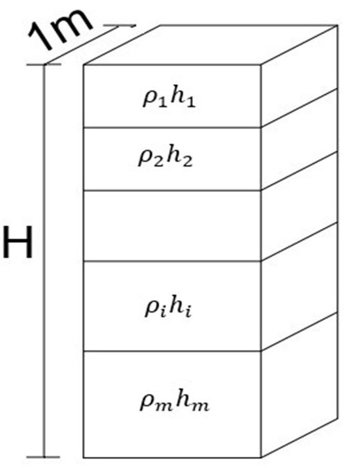
DAR ZARROUK PARAMETERS

Transverse Resistance B.4 ∗ =∑ Transverse Resistivity B.5 = ∗ = ∑ ∑ Longitudinal conductance B.6 ∗ =∑ Average longitudinal conductivity B.7 = ∗ = ∑ ∑

Coefficient of Anisotropy B.8 = = ∗ ∗ = ∑ ∑ (∑ )

E potential gradient resistivity j current density resistivity of fluid and grains ρw resistivity of pore fluid a coefficient m coefficient Ff formation factor T∗ transverse resistance i layer number m maximum number of layers transverse resistivity

S∗ longitudinal conductance average longitudinal resistivity coefficient of anisotropy

Fig: 1. The Dar zarrouk parameters (after Maillet, 1947)

ISSN: 2321 9653; IC Value: 45.98; SJ Impact Factor: 7.538 Volume 10 Issue XI Nov 2022 Available at www.ijraset.com

C. Petrophysics And Hydrology

Most scientists observe an exponential relationship between intrinsic permeability and porosity

C.1 = ∅ C.2 = ∅ From Archie’s Law: B.2 = ∅ Ff = ,∅ w= constant = ∅ ∅ = ∅ = = =

In Southern Illinois (from Heigold et.al., 1979) (K in cm/sec) = . , = 386.40 ℎ

For granular aquifers: ’ = , = . So and h must be determined separately. To determine the difficulties in doing this, one must review the theory behind electrical soundings.

D. Surficial Resistivity

a) Electrical behavior around a PointSource D.a.1 E = Ohm’s law D.a.2 ∆. j = (Divergence = 0) All current leaves unless there is a source or sink. Combine to obtain Laplace’s equation. D.a.3 = ∆ = ∆ = = (From D.a.1, D.a.2) In polar coordinates this becomes: + + + = Because we are concerned with homogeneous, isotropic conditions: = Integrating twice gives: D.a.4 = + b.c. r→ ∞, = 0 ∴ = 0 Use divergence theorem to solve for C. D.a.5 = = = (From D.a.3, D.a.4) =∫ =∫ =∫ (From D.a.1, D.a.5) = = D.a.6 = , = = (From D.a.4) E potential grade r radius of area j current density s surface U variable such that E is its grade

Journal for Research in Applied Science & Engineering Technology (IJRASET

ISSN: 2321 9653; IC Value: 45.98; SJ Impact Factor: 7.538 Volume 10 Issue XI Nov 2022 Available at www.ijraset.com

b) Homogeneous Anisotropic Earth Potential

D.b.1 = + + = + + =

Stetch anisotropic space into isotropic space = = =

D.b.2 = 2 + 2 + 2 This equation becomes Laplace’s equation D.b.3 = = (From D.b.1, D.b.2) D.b.4 = + b.c. R→ ∞, =0, ∴ = 0

Solve for, using divergence theorem: = = (From D.b.2, D.b.4) = = = = D.b.5 | |=( + + )1/2 = D.b.6 x 2+y2=R2sin2θ Z=R2cosθ (From D.b.5, D.b.6) | |= = =∫ | | =∫ ∫ | | Ψ

D.b.7 I= (From Keller and Frichknecht, 1966) D.b.8 U= I (From D.b.4) = = (For a single pole array) (From D.b.6) Anisotropy makes determination of difficult. c) More than one current source

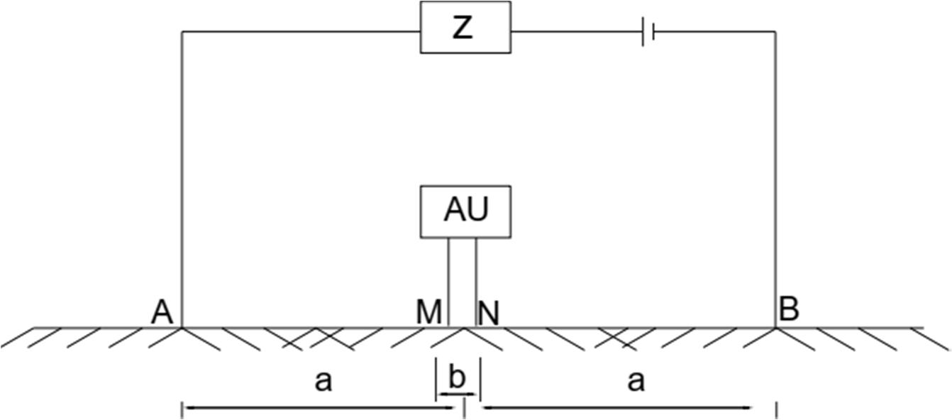
Fig: 2.Configuration of the Schlumberger electrode array

ISSN: 2321 9653; IC Value: 45.98; SJ Impact Factor: 7.538 Volume 10 Issue XI Nov 2022 Available at www.ijraset.com

With several sources of current use image theory. = + + +⋯ (From D.a.6)

D.c.1 = = ∆

K’ called geometric factor. d) Boundary plane effects

Fig.3

Consider now an optical analogy to the electrical problem described by figure (Fig.3). The source of current at A is replaced with a light source, and the boundary is replaced by a mirror with a reflection coefficient, K, and a transmission coefficient, I K. If the light is viewed from point M1 on the top side of the mirror, the original source is seen with its full intensity, and in addition, an image source is seen reflected from the mirror. This image source appears to be located behind the method at a distance, h, and has intensity I1.

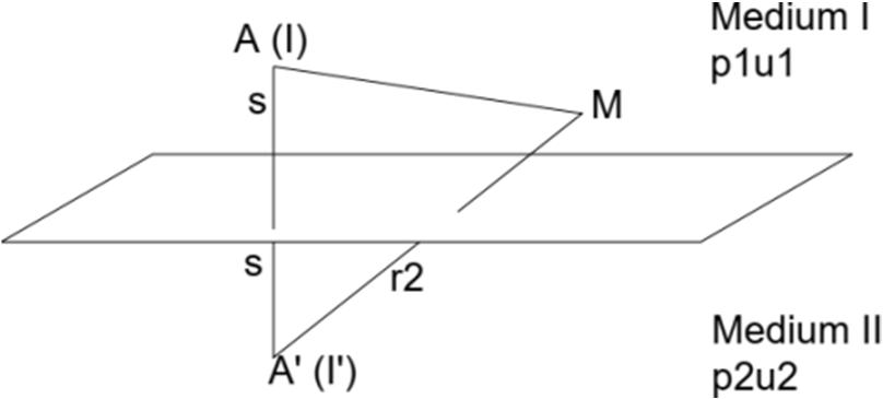
Use optical analogy current source at A replaced by a mirror with reflection coefficient K and a transmission coefficient, of (1 K).

At M: = + (From D.b.6) D.d.1 = = , 1, Z = reflection coefficient for boundary when viewed form medium I.

e) For a single overburden

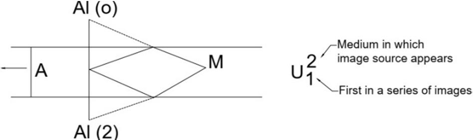
If each of the boundary plane is replaced with semi transparent mirror, with reflection coefficients, an observer at the point M will see images of the primary source reflected from both the upper and lower boundaries. The apparent intensity of the upper image source is IK1, 0, where K 1, 0 is the reflectivity of the upper plane when viewed from underneath. The apparent intensity of the lower image source is IK1, 2, where K1, 2 is the reflectivity of the lower plane viewed from above. The contributions to the potential function at the point M from these images (Fig.4)

Where the superscript refers to the medium in which the image source appears to be and the subscript indicates that this is the first in a series of images. The image series comes about since in the optical there is no limit to the number of images formed by multiple reflections of light rays between the two mirrors. Considering first only the paths in which the first bounce is off the lower plane, we can examine the behavior of images for multiple reflections. For a path with one reflection from each plane, the image source appears to be in medium O, and has intensity IK1,2 K1,0. The contribution to the total potential at point M from this image. The ray path with two reflections each from the upper and lower planes. The image strength is reduced on each reflection by the corresponding reflection coefficient, so the image strength is IK2 1,2 K2 1,0. The image appears to be a distance 2t further above the top plane than the preceding image. The contribution to the potential at M due to this image (Fig.4)

ISSN: 2321 9653; IC Value: 45.98; SJ Impact Factor: 7.538 Volume 10 Issue XI Nov 2022 Available at www.ijraset.com

K1,0 = Reflectivity of Upper plane when viewed from underneath U at M = ( ) + ( ) + ( ) + D.e.1 ( ) = , ( ) = ( )

f) For n number of boundary planes the total potential function becomes: D.f.1 = + ∑ , (From D.e.1) (Keller and Frischknet, 1966)

Normal Potential Disturbing potential

The Schlumberger electrode spread measures potential gradient The derivative is doubled because there are two current electrodes. The apparent resistivity is then: D.f.2 = = + ∑ , (From D.f.1) If a<<t: → = t = layer thickness If a>>t: D.f.3 → = ∑ , = + ( ) D.f.4 → = ⎣ ⎢ ⎢

g) Reflection coefficient equal to one

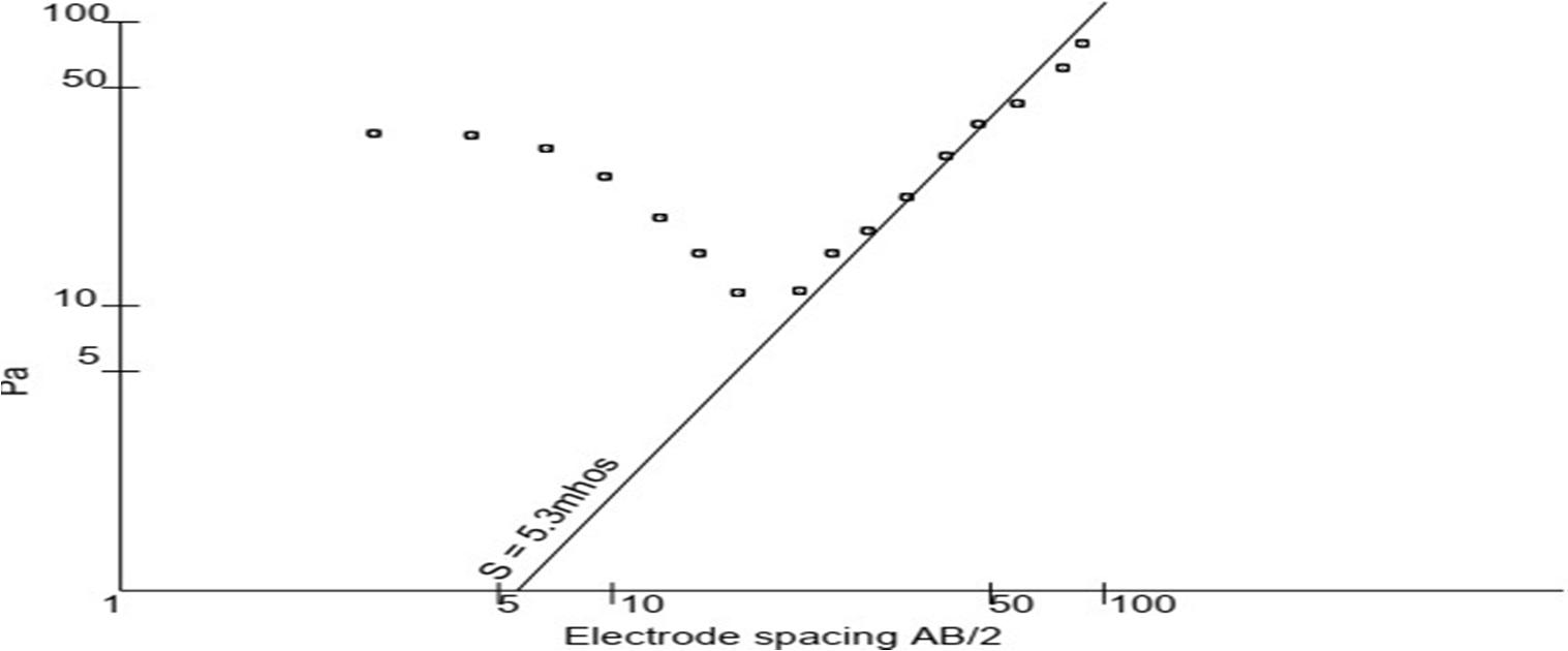
When K is equal to one, as often is the case with alluvial aquifers in nature, no current can pass into the insulating lower layer. Use of an array where the measurements are made midway between two widely spaced electrodes, yields a doubling of the electrical field. These conditions are met with the Schlumberger array. D.g.1 = (From D.a.6, a = radius, t = height) Therefore, when K = 1: D.g.2 = = (From D.a.5, D.a.6) D.g.3 = (From D.g.1, D.g.2) D.g.4 = = ∗ (From D.g.3)

The relationship between a and is linear with a slope of one. Extrapolating the 450 portion of the curve yields ∗

Fig: 5 Interpretation of two layer curves using the method of asymptotes (From Keller and Frischknecht, 1966)

ISSN: 2321 9653; IC Value: 45.98; SJ Impact Factor: 7.538 Volume 10 Issue XI Nov 2022 Available at www.ijraset.com

E. Relationships Between Hydrogeology And Dar Zarrouk Parameters

In order to correlate electrical parameters with Hydrogeological properties, a correction for variations in must be made. One way to do this is to measure for wells and low flow streams throughout the study area, then inter polate the results to the specific sounding sites. Dividing T* and multiplying S* by values for gives us the corrected parameters:

E.1 ∗ = ∗ , ∗ = ∗

If there is little contrast between the resistivity of the matrix and pore fluids, then a correction must also be made for matrix conduction. Worthington (1975) has derived an expression for this: ∗ = ∗( ) ( )

E.2 ∗ = ∗( ) ( )

b = depth averaged matrix conduction parameter

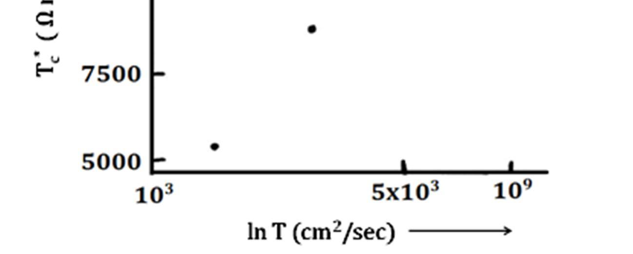
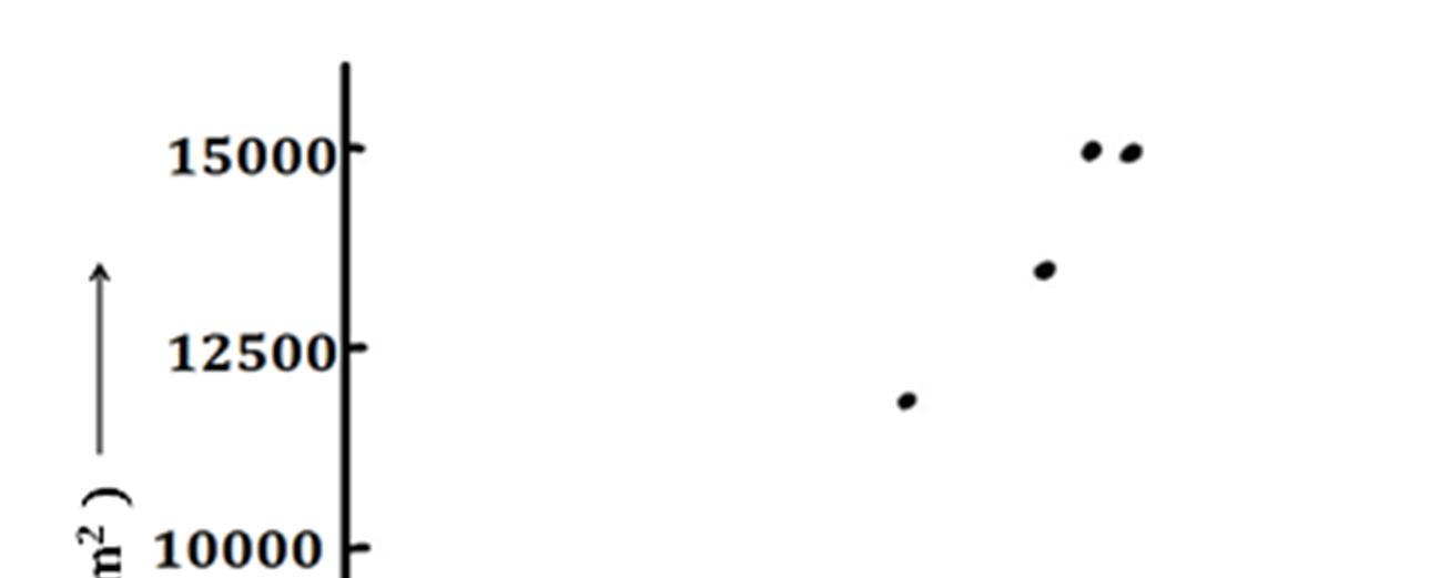
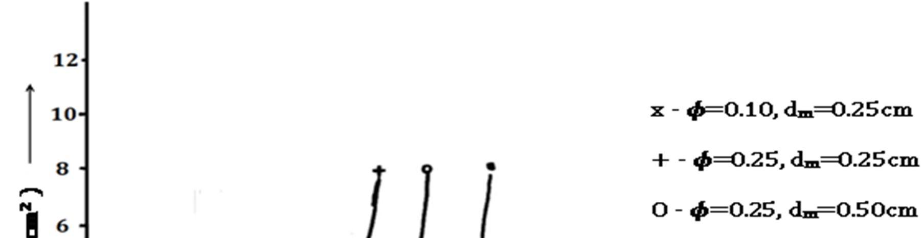
Duprat et al (1970) noted an empirical semi logarithmic relationship between T and T* for granular deposits of the Rhine alluvial plain (see Figure 6). Values of a, b, θ and dm corresponding to fine sand and silt may be inserted into Archie's formula and the Kozeny Carmen equation to derive K and ρ. These parameters may be multiplied by arbitrary thicknesses to obtain values of T and T* respectively. Assuming that this theoretical T* equals Tc * , and plotting the In of T against Tc * such as Duprat did, yields an exponential curve with the tail resembling a straight line (see Figure 7). Plotting ln T versus In Tc * yields a linear relationship with a slope of one. The intercept of the y axis, B, is dependant upon the porosity and mean grain size. It appears then, that Duprat's field data did not include sites with small enough values of T and Tc * to reach the bend in the exponential curve. A more appropriate expression for the relationship between T and Tc * would be:

E.3 ∗ = + ∗ =

Where B is a variable depending on the physical characteristics of a particular aquifer. Similarly a relationship between T and Sc * may be derived: ∗ = + ∗ =

E.4 T = ∗

Fig. 6 (From DUPRAT, 1970)

International Journal for Research in Applied Science & Engineering Technology (IJRASET)

ISSN: 2321 9653; IC Value: 45.98; SJ Impact Factor: 7.538 Volume 10 Issue XI Nov 2022 Available at www.ijraset.com

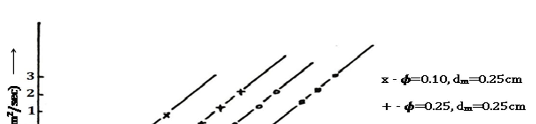
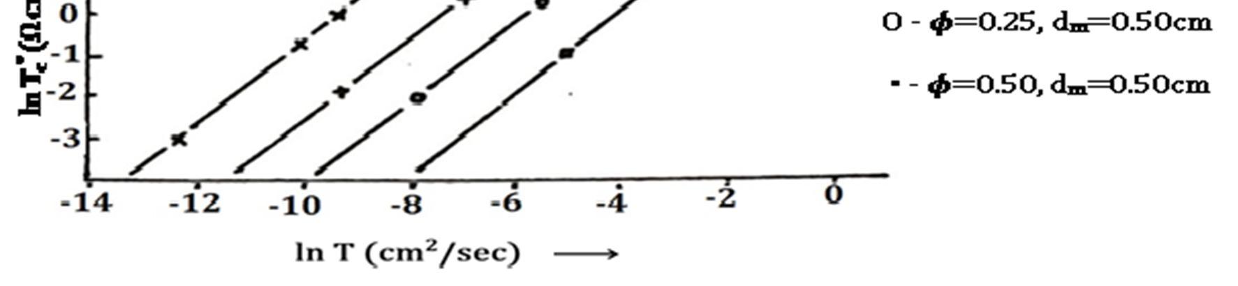
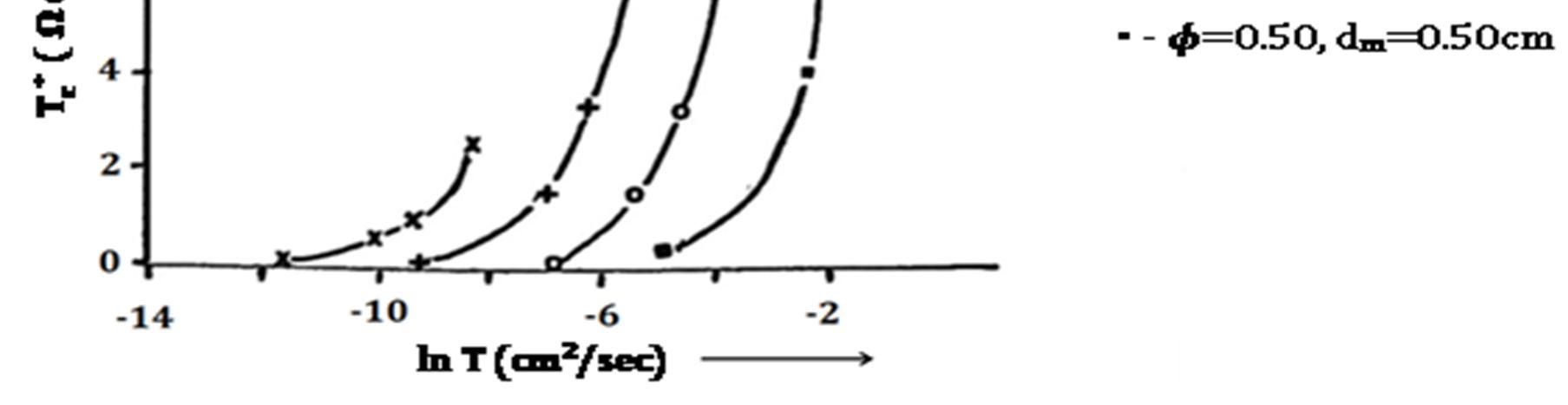
Fig.7 Fig.8 Fig.9

ISSN: 2321 9653; IC Value: 45.98; SJ Impact Factor: 7.538 Volume 10 Issue XI Nov 2022 Available at www.ijraset.com

Once again, the value, A, depends on the properties of the particular aquifer under consideration. Hydrogeophysical relationships involving S* are probably the most useful in dealing with granular aquifers, because the aquifer bedrock reflection coefficient is often one, in this case.

Henriet (1976) cites several other applications of longitudinal conductance to aquifer studies. Clays are in general excellent conductors, and S* for a clayey layer should be large. Henriet was studying a limestone aquifer overlain by clay. He mapped S* for the layers above the aquifer in order to obtain a comparative measurement of protection of the aquifer throughout the study area. This was in order to pinpoint sites susceptible to contamination. Henriet then used Nechai's (1964) equation relating the rock matrix resistance, , , and joint porosity Φ E.5 = Φ + ( Φ) Φ

As the resistivity of the limestone is very high, the second term, may be neglected. = Φ

Developing the expression for Sc * for the aquifer (the nth layer) leads to an expression whereby the thickness is multiplied by Φ. This product is the volume of water dW, in an aquifer column of unit cross section area. E.6 ∗ = = = (from E.5, B.6) d = . ∗ A relationship such as this is not as easy to derive for granular aquifers because the correlation between ρ and ᴓ is exponential according to Archie's law. However if h and ρw can be estimated at sites throughout the area, an expression for dW may be derived: E.7 ∗ = = ∅ (from B.2, B.6) ∗ = ∅ (From E.1, E.7) ∗ = + ∅ ∗ = ∅ ∗ =∅ = ∗ =

II. CONCLUSION

In conclusion, the use of the Dar Zarrouk parameters may be an important tool in determining an aquifer's hydrogeologic characteristics. Difficulties in using these parameters may be due to matrix conductance or sudden simultaneous changes of ρw, ᴓ and h of the aquifer in question. Their main advantage is that when used under the proper conditions, they eliminate the need for complicated interpretation of electrical soundings to determine ρ and h.

REFERENCES

[1] Chen J, Hubbard S, Rubin Y.,2001. Estimating the hydraulic conductivity at the south Oyster site from geophysical tomographic data using Bayesian techniques based on the normal linear regression model. Water Resources Research, 37(6): 1603 1613.

[2] Duprat, A., Simler, L., and Ungemach, P., 1970. Pub. No. DC 70 03: Compagnie Generale de Geophysique, Paris.

[3] Frolich RK, Kelly WE., 1988. Estimates of specific yield with the geoelectrical resistivity method in glacial aquifers. J. Hydrology, 97: 33 44.

[4] Frolich RK, Urish D., 2002. The use of geoelectrics and test wells for the assessment of groundwater quality of a coastal industrial site. J. Applied Geophysics, 50: 261 278

[5] Heigold, P.C., Gilkenson, R.H., Cartwright, K., and Reed, P.C., 1979. Aquifer transmissivity from surficial electrical methods: Illinois State Geological Survey Report of Investigations No. . 23 p.

[6] Henriet, J.P., 1976. Direct applications of the Dar Zarrouk parameters in groundwater surveys: Geophysical Prospecting 24, 344 353.

[7] Huntley D., 1986. Relations between permeability and electrical resistivity in granular aquifers. Ground Water, 24: 466 474.

[8] Kalinski KJ, Kelly WE, Bogardi I., 1993. Combined use of geoelectric sounding and profiling to quantify aquifer protection properties. Ground Water, 31 (4): 538 544.

[9] Keller, G.V. and Frischknecht, F.C., 1966. Electrical Methods in Geophysical Prospecting, chapter 3. London, Pergamon.

[10] Kelly, W.E., 1977. Geoelectric sounding for estimating aquifer hydraulic conductivity. Ground Water,15: 420 425

[11] Kosinki WK, Kelly WE., 1981. Geoelectric sounding for predicting aquifer properties. Ground Water, 19 (2): 163 171

[12] Lashkaripour GR., 2003. An investigation of groundwater condition by geoelectrical resistivity method: a case study in Krin aquifer southeast Iran. J. Spatial Hydrology, 3 (1): 1 5

[13] Louis IF, Karantonis GA, Voulgaris NS, Louis FI., 2005. The contribution of geophysical methods in the determination of aquifer parameters: the case of Mornos River Delta, Greece. Department of Geophysics and Geothermic, University of Athens, Greece. 41pp

[14] Mazac O, Kelly WE Landa I., 1985. A hydrogeophysical model for relations between electrical and hydraulic properties of aquifers. J. Hydrol. 79: 1 19

(IJRASET

ISSN: 2321 9653; IC Value: 45.98; SJ Impact Factor: 7.538 Volume 10 Issue XI Nov 2022 Available at www.ijraset.com

[15] Niwas, S. and Singhal, D.C., 1981. Estimation of Aquifer Transmissivity from Dar Zarrouk Parameters in Porous Media

[16] Onuoha KM, Mbazi FCC., 1988. Aquifers transmissivity from electrical sounding data: the case of Ajali sandstone aquifers southwest of Enugu, Nigeria. In Ofoegbu CO (ed). Groundwater and mineral resources of Nigeria. Vieweg Verlag, 17 30

[17] Schimschal U.,1981. The relationship of geophysical measurements to hydraulic conductivity at the Brantley dam site, New Mexico. Geoexploration. 19: 115 125

[18] Singh KP., 2005. Nonlinear estimation of aquifer parameters from surficial resistivity measurements. Hydrol. Earth Sys. Sci. Discuss. 2: 917 938.

[19] Urish DW., 1981. Electrical resistivity hydraulic conductivity relationships in glacial outwash aquifers. Water Resour. Res. 17(5): 1401 1408

[20] Worthington, P.F., 1975. Quantitative geophysical Investigations of granular aquifers: Geophysical Surveys 2, no. 4, 313 366.